Ising films with surface defects

Abstract

The influence of surface defects on the critical properties of magnetic films is studied for Ising models with nearest-neighbour ferromagnetic couplings. The defects include one or two adjacent lines of additional atoms and a step on the surface. For the calculations, both density-matrix renormalization group and Monte Carlo techniques are used. By changing the local couplings at the defects and the film thickness, non-universal features as well as interesting crossover phenomena in the magnetic exponents are observed.

I Introduction

Critical phenomena of magnetic films are of current interest, both experimentally and theoretically [1, 2, 3, 4, 5]. In the limiting cases of one layer and of infinitely many layers, one deals with two-dimensional magnets [6] and with standard bulk and surface magnetism [7, 8, 9, 10], respectively. For systems consisting of a finite number of layers, interesting crossover phenomena between these limiting cases are expected.

In this article, we shall consider critical properties of ferromagnetic films of Ising magnets with various imperfections at the surface, motivated partly by possible experimental realizations of magnetic thin films with stripes of magnetic adatoms and stepped surfaces [1, 11, 12], partly by genuine theoretical interest. Imperfections may be due to regular or irregular changes in the surface couplings or due to additional structures on the surface. A simple example of the first case is a ladder of modified couplings in an otherwise uniform two-dimensional system as introduced by Bariev [13], see Fig. 1(a). We will study this briefly, since it can serve as a testing ground. Our main interest, however, is in additional structures, as depicted in Figs. 1(b)–(d). Thus we will investigate surfaces with magnetic adatoms in the form of

• one additional straight line, Fig. 1(b),

• two neighbouring lines, Fig. 1(c),

• a straight step of unit height, Fig. 1(d),

for various local couplings at the defects and for films of varying thickness.

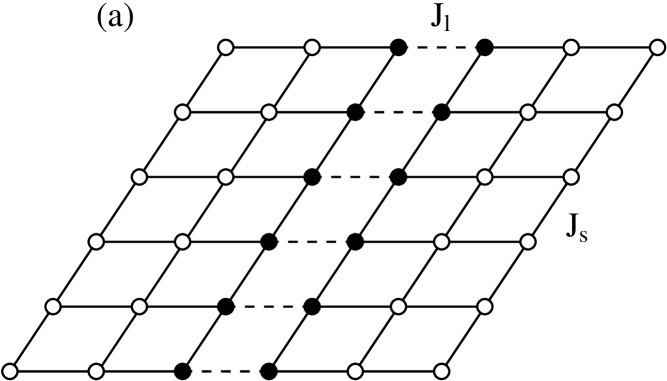
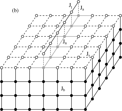
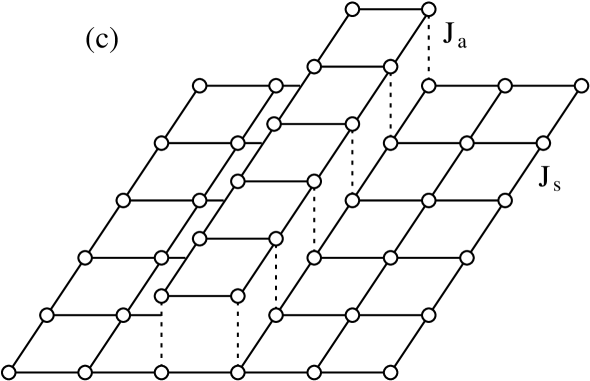
FIG. 1.: Geometry and interactions of Ising models with various surface imperfections: (a) ladder defect, (b) one additional line of spins, (c) pair of adjacent lines of magnetic adatoms, and (d) straight step of monoatomic height. Usually, surface spins are denoted by open circles, and bulk spins by full circles. In case 1(b), the shaded spins allow for both interpretations.

Previous related work on Ising models includes the study of the step magnetization at the ordinary transition of rather thick films [14] and the study of magnetism in thin films with rough surfaces [15].

In studying the influence of these imperfections especially on the critical behaviour, we use the density- matrix renormalization group technique (DMRG) [16, 17], being most suitable in the case of merely one layer, and the Monte Carlo (MC) method [18], which allows to treat films of considerable thickness as well.

The article is organized as follows. In the next section, we present our findings on single layers with defects, applying DMRG. The MC results on single layers and on films with an additional line of magnetic adatoms and with a straight step on top of the surface are discussed in Section 3. A short summary concludes the article.

II One layer: DMRG

The planar Ising model with line-like defects is a peculiar system, because it shows non-universal magnetic exponents. This is connected with the values $\nu=1$ and $x_{s}=1/2$ of the exponents for the correlation length and the surface magnetization of the pure system, respectively. A one-dimensional, energy-like perturbation then is marginal and can change the critical behaviour continuously. For this reason, the system has been the topic of various studies [6], with the focus most recently on a conformal treatment [19] and on random systems [20]. While the simple chain and ladder defects considered by Bariev are solvable free-fermion problems, the other cases we study are not integrable and one has to use numerical methods. In the following we dicuss the quantity of direct physical interest, the local magnetization at or near the defect lines.

To obtain it, we used the transfer matrix running along the direction of the defect, see Figs. 1(a)–(c), and determined its maximal eigenvector via the DMRG method [21]. In this way one is treating an infinitely long strip of width $M$ with the defect located in the middle. Only the infinite-system algorithm was used, in which one enlarges the system step by step and always chooses an optimal reduced basis via the density matrix. This is very convenient, since one can insert different defects after the system has reached the desired size. No further sweeps to optimize the state were made, since tests on the ladder defect gave very good results without them. Most calculations were done with $64$ kept states and a truncation error around $10^{-15}$. The local magnetization $m(i)$ was determined from the spin correlation function $C(i)=\langle\sigma_{1}\sigma_{i}\rangle$ for free boundary conditions, or directly as $\langle\sigma_{i}\rangle$ for fixed boundary spins. The width was always much larger than the correlation length and varied between $M=100$ and $M=5000$ for the temperature range studied ($0.001<t<0.1$, where $t=1-T/T_{c}$ is the reduced temperature). The (absolute) error in $m$, determined by comparing with anaytical results was at most $10^{-4}$ for a system at $t=0.001$, cut in the middle by a ladder defect. For less severe modifications and larger values of $t$ it was even smaller.

FIG. 2.: Spin correlation function $C(i)$ for a strip of width $M=150$ with ladder defects (below the plateau) or one additional line of spins (above the plateau), as obtained from DMRG calculations at the reduced temperature $t=0.072$. The defect strengths $J_{l}/J_{s}$ and $J_{a}/J_{s}$ are indicated. Upper part: total view, lower part: central region.

In Fig. 2 we show the correlation function $C(i)$ across the strip for ladder defects (Fig. 1(a)) and for an additional line (Fig. 1(b); in the DMRG study we considered the case $J_{n}=J_{s}$). The upper part gives an overall picture, while the lower one shows the defect region in more detail. For ladder defects the strength $J_{l}$ of the defect bonds was varied, whereas for an additional line it was the coupling $J_{a}$ between the line spins and the substrate. Since $C(i)$ factors for large distances, these curves also give the profile of the magnetization in the bulk. One can see how $m$ increases or decreases near the defect, depending on the sign of the perturbation (similar curves were obtained in [20] for a random system). If one cuts the ladder bonds by choosing $J_{l}=0$, one obtains the boundary magnetization of the homogeneous model in the middle of the strip. On the upper side, the possible increase of $m$ depends on the details of the defect. It is limited if one varies $J_{a}$, because a line with infinite $J_{a}$ is equivalent to a chain defect in the plane with merely doubled bond strength.

The temperature dependence of $m$ is shown in Fig. 3 for the spins in the plane situated below one or two additional lines. One can see how it is increased over the Onsager value by increasing the coupling $J_{a}$. As expected, the effect is even stronger for two additional lines. In this case, $m$ has already twice the undisturbed value for the smallest shown $t$. Quantitatively, this enhancement is described by a decrease of the exponent $\beta_{l}$, the local critical exponent which describes the vanishing of the magnetization near the additional line of magnetic adatoms.

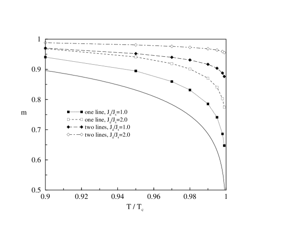
FIG. 3.: Local magnetization $m$ of the spins below one or two additional lines as a function of temperature, for three values of the coupling ratio $J_{a}/J_{s}$. The lowest curve is the Onsager result for the perfect Ising model.

To investigate this, we have analyzed the temperature behaviour of $m$ in terms of an effective (critical) exponent $\beta_{eff}$, defined by[2, 14, 22]

$$\beta_{eff}(t)\;=\;\ln(m(t_{i})/m(t_{i+1}))/\ln(t_{i}/t_{i+1})$$ (1)

with $t=(t_{i}+t_{i+1})/2$ (alternatively, one could choose $t$ to be the geometric mean $t=\sqrt{t_{i}t_{i+1}}$). As one approaches the critical point, $t\rightarrow 0$, this quantity converges to the true local exponent $\beta_{l}$. It is also a very sensitive indicator for the numerical accuracy of a calculation.

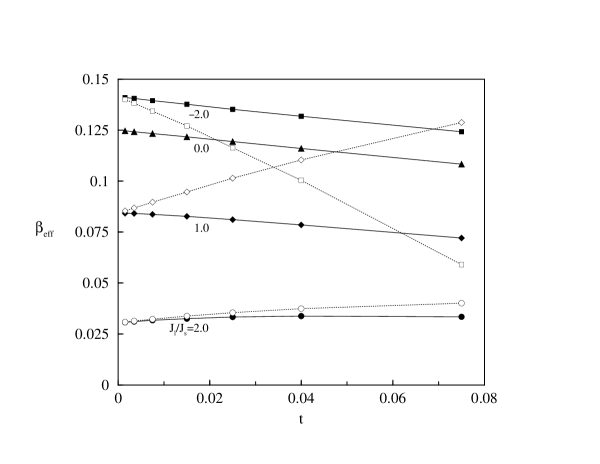
FIG. 4.: Effective exponent $\beta_{eff}$ as function of the reduced temperature $t$ for one additional line and three different coupling ratios $J_{l}/J_{s}$. Full: Spins located below the line, dotted: spins in the line.

Some typical results are given in Fig. 4 for one additional line and four values of the ratio $J_{l}/J_{s}$ of the couplings in the line. For $J_{l}$ = 0, one is treating the plane with independent attached spins and the Onsager result $\beta=0.125$ is recovered with high accuracy. In the other cases, the exponents both for the spin in the line and the one below it are shown and one sees that the two curves have different slopes, but a common limit for $t\rightarrow 0$ which can be determined very precisely. The values for $\beta_{l}$ found in this way are accurate to at least three digits. For the case $J_{a}/J_{s}\gg 1$ which, as mentioned, is equivalent to a line defect in the plane, this was checked explicitely by comparing with the analytical result. In the figure, also a negative $J_{l}$ is shown, which leads to a reduction of $m$ and an increase of $\beta_{l}$ over the Onsager value . In this case, a limiting value $0.142$ is approached rapidly for $J_{l}/J_{s}<-1$. This is the same effect as for a chain defect in the plane with strong antiferromagnetic couplings [6]. In that case, the exponent is increased up to the value 0.5 of the free surface. The sign of $J_{a}$, on the other hand, has no influence on the exponent.

The results for $\beta_{l}$ are collected in Table 1 and in Fig. 5, where the exponent is plotted as a function of the varied couplings (keeping the other couplings fixed and equal to $J_{s}$). For comparison also the analytical results [13, 6], for simple chain and ladder defects are shown in Fig. 5. One notes that, for a single line and small modifications, it does not matter much whether one changes $J_{a}$ or $J_{l}$. A large $J_{l}/J_{s}$, however, has a much more pronounced effect than $J_{a}/J_{s}$, since it corresponds to additional spins which are almost rigidly locked together. For the double line, the exponent drops much faster, reaching $10^{-2}$ already around $J_{a}/J_{s}\sim 1$. For more additional lines, i.e. for a terrace on the surface as in Fig. 1(d), this effect would be even stronger. In this case, the magnetization would practically jump as in a first-order transition.

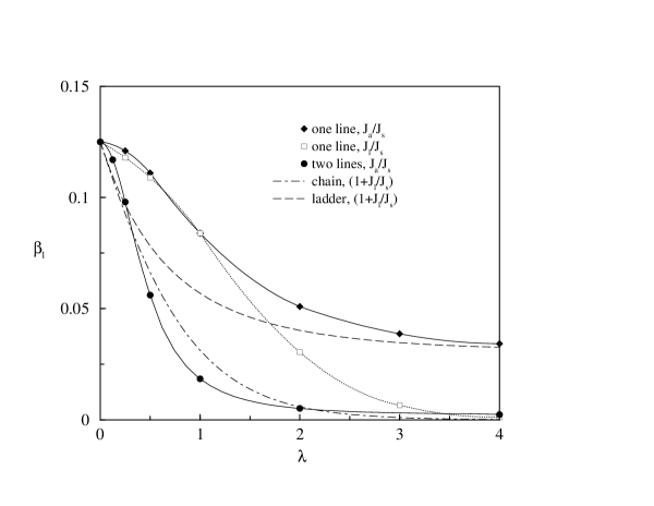
FIG. 5.: Local exponent $\beta_{l}$ as a function of the ratio of the coupling strength $\lambda$, as defined in the figure for five different situations. For chain and ladder defects the analytical results are shown, otherwise the DMRG results are depicted.

TABLE I.: Numerical values for the local exponent $\beta_{l}$ of an Ising plane with one and two additional lines of spins.

lines	1	1	2
$\lambda$	$J_{a}/J_{s}$	$J_{l}/J_{s}$	$J_{a}/J_{s}$
$0.0$	$0.125$	$0.125$	$0.125$
$0.25$	$0.121$	$0.118$	$0.098$
$0.5$	$0.111$	$0.109$	$0.056$
$1.0$	$0.084$	$0.084$	$0.018$
$2.0$	$0.051$	$0.031$	$0.005$
$4.0$	$0.034$	$0.002$	$0.001$

III Films: Monte Carlo simulations

A One additional line of spins

Extending the DMRG calculations on an Ising layer with one additional line of spins, we did Monte Carlo simulations on the corresponding Ising films, consisting of $L$ layers with one line of magnetic adatoms on top of the surface, see Fig. 1(b). We set $J_{l}=J_{s}$, with $J_{a}=J_{n}=J_{s}$ (variant A, treating the spins directly below the additional line as surface spins, as it was done in the DMRG study) or $J_{a}=J_{n}=J_{b}$ (variant B, treating the spins directly below the additional line as bulk spins).– In the layers, periodic boundary conditions are used.

Let $S_{i,j,k}=\pm 1$ be the spin on site $(i,j)$ in the $k$th layer. Taking layers of $M\times N$ spins, the spins in the additional line on top of the surface through the center are located at $(i=(M+1)/2,j,k=0)$, $M$ odd, with $j$ running from 1 to $N$. We computed, among others, the line magnetization $m(i,k;L)$ defined by

$$m(i,k;L)=\frac{1}{N}\left<\left|\sum\limits_{j}S_{i,j,k}\right|\right>$$ (2)

The magnetization of the line on top of the surface, $m_{l}$, is given by $m_{l}(L)$= $m((M+1)/2,k=0;L)$.

In the simulations, the film thickness $L$ ranged from 1 to 40, with layer sizes being sufficiently large to circumvent finite–size effects (up to $161\times 320$). To speed up computations, the single–cluster–flip algorithm was implemented. We studied the cases (i) $J_{s}=J_{b}$ as well as (ii) $J_{s}=2J_{b}$ (variants A and B), which lead to the two characteristic scenarios of surface critical phenomena for $L,M,N\rightarrow\infty$ (semi–infinite case). In the first case, bulk and surface spins order simultaneously at temperature $T_{c}$ (ordinary transition), while in the second one the surface spins order at a higher temperature, $T_{s}$ (surface transition) [7, 8].

(i) At the ordinary transition of the semi–infinite Ising model, $L\rightarrow\infty$, the magnetization deep in the bulk vanishes like $m\propto t^{\beta}$, with $t=|T-T_{c}|/T_{c}$, where $\beta=0.31...$ [23, 24]. At the perfect, flat surface, one finds $m\propto t^{\beta_{1}}$, with $\beta_{1}\approx 0.80$ [25, 14]. The vanishing of the magnetization in the additional line of spins on top of the surface is expected to be governed by $\beta_{1}$ as well, i.e. $\beta_{l}(L\rightarrow\infty)=\beta_{1}$ [14, 26]. On the other hand, for a single perfect layer, $L=1$, it is well known that $m\propto t^{\beta_{2d}}$, $\beta_{2d}=1/8$. Adding a row of spins, we obtain, from the DMRG calculations, $m_{l}\propto t^{\beta_{l}(L=1)}$ with $\beta_{l}(L=1)\approx 0.084$, see Table 1.

To monitor the influence of the layer thickness $L$ at the ordinary transition, we computed magnetization profiles $m(i,k;L)$, the critical temperature $T_{c}(L)$, and the critical exponent $\beta_{l}(L)$. The dependence of the transition temperature on the thickness $L$ has been studied before for flat films [7, 15], and it is, certainly, not affected by the presence of the additional line. In Fig. 6, the magnetization in the defect line, $m_{l}(L)$, is depicted as a function of temperature for $L$ ranging from 1 to 5, illustrating the increase of the transition temperature with $L$. In the ordered phase, $T<T_{c}$, the line magnetization $m(i,k;L)$ is, in each layer, maximal for the center line, $m((M+1)/2,k;L)$, see also Fig. 2. The maximum is most pronounced at $k=1$ (we shall denote the magnetization in that line beneath the additional row of spins by $m_{lb}=m((M+1)/2,1;L)$), due to the increased coordination number, compared to the other surface lines. The magnetization in the additional line, $m_{l}$, is suppressed compared to $m_{lb}$, because of missing neighbouring spins.

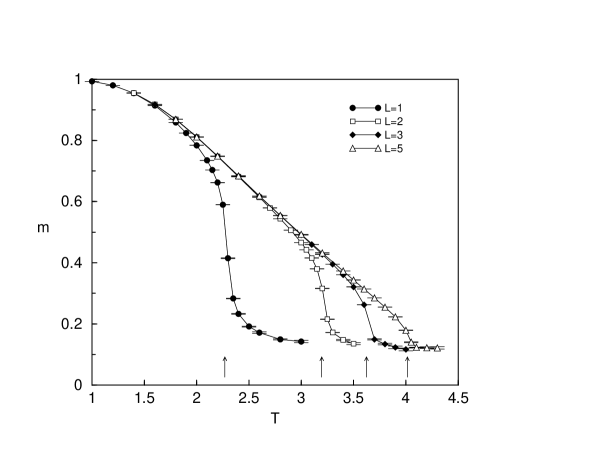
FIG. 6.: Simulated magnetization in the additional line $m_{l}(L)$ for Ising films with $L$ layers and one additional line of spins on the surface, choosing $J_{s}=J_{b}$, for $L$ ranging from 1 to 5. Each layer consists of $81\times 80$ spins. The critical temperatures $T_{c}(L)$ are marked by arrows.

Various crossover effects show up in the effective exponent $\beta_{eff}(i,k;L)$, defined by $m(i,k;L)\propto t^{\beta_{eff}(i,k;L)}$, corresponding to the slope in a standard log–log–plot of the temperature dependence of the magnetization [2, 14, 22], see eq. (1). On approach to $T_{c}$, one expects to observe the limiting cases $\beta_{eff}(i,k;L)\rightarrow\beta$ for $k$ and $L$ large, $\rightarrow\beta_{1}$ for $k$ small and $L$ large, $\rightarrow\beta_{l}(L=1)$ for $L=1$ and $i=(M+1)/2$, $k=0$ or 1, and $\rightarrow\beta_{2d}$ for $L=1$ and sufficiently far away from the additional line in the centre.

The crossover behaviour is illustrated in Fig. 7, showing $\beta_{eff}((M+1)/2,k;L)$ for $m_{l}(L)$, $k=0$, and $m_{lb}(L)$, $k=1$, with the film thickness ranging from $L=1$ to 10. $\beta_{eff}((M+1)/2,0;L)$ decreases monotonically, except for $L=1$, over a wide range of temperatures on lowering $t$, but with the effective exponent, at fixed $t$, increasing clearly with the film thickness, as depicted in Fig. 7(a). The data seem to indicate that the asymptotic critical exponent $\beta_{l}(L)$, as $t\rightarrow 0$, of the magnetization in the additional line of magnetic adatoms increases, however, only weakly with $L$, being quite small, around 0.1, for $L$ going up to 10 (the increase itself may be argued to reflect the diminishing role of the defect line on the two–dimensional critical fluctuations in thicker films; of course, $\beta(L)$ is bounded by 1/8 for finite $L$). For the magnetization beneath the additional line, $m_{lb}$, corrections to the asymptotics are rather large as well, see Fig. 7(b). Here the effective exponent $\beta_{eff}((M+1)/2,1;L)$ changes with temperature in a non–monotonic fashion, except for $L=1$. In agreement with the observations for $m_{l}$, the true critical exponent $\beta_{l}(L)$ is rather small, around 0.1, increasing only weakly with $L$. The location of the maximum in $\beta_{eff}((M+1)/2,1;L)$ indicates the temperature, at which one crosses over from the regime dominated by two–dimensional critical fluctuations, close to the phase transition, to the regime, further away from the critical point, where the fluctuations are (nearly) isotropic and three–dimensional. Thence, at the maximum the corresponding correlation length is argued to be about the thickness of the film $L$. In the thermodynamic limit, $L\rightarrow\infty$, the maximum is believed to shift towards $t=0$, with its height being $\beta_{l}=\beta_{1}\approx 0.80$.

Note that the strong corrections to scaling, as seen by the deviations of the effective exponents from their asymptotic values, may cause severe difficulties in extracting the true critical exponents in simulations as well as in experiments.

Similar crossover phenomena, now between $\beta_{2d}$, $\beta_{1}$ and $\beta$, are expected to occur for the magnetization far away from the defect line, when varying the film thickness. This aspect, however, is of minor importance in the context of this study.

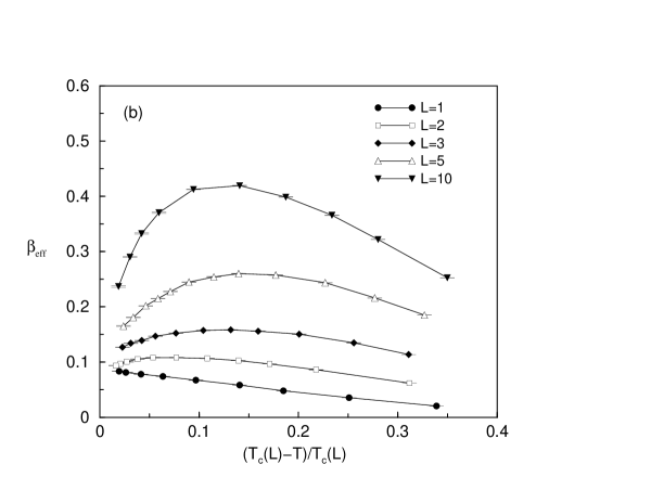
FIG. 7.: Effective exponent $\beta_{eff}((M+1)/2,k;L)$ of the magnetization (a) in the additional line of spins ($k=0$), $m_{l}$, and (b) in the line beneath ($k=1$), $m_{lb}$, for the Ising model with equal couplings, as obtained from the MC simulations. The sizes of the layers are up to $161\times 320$ spins. Only results which are essentially free of finite–size effects are shown.

(ii) At the surface transition of flat Ising films, the surface magnetization vanishes, on approach to $T_{s}$, like $m\propto t^{\beta_{2d}}$, independent of $L$. The critical exponent for the magnetization at the additional line of magnetic atoms on top of the surface, $\beta_{l}$, with $m_{l(lb)}\propto t^{\beta_{l}}$, depends on the local couplings at that line, as seen from our DMRG results for $L=1$. Indeed, the situation is similar to that of the edge magnetization at the surface transition, the edge corresponding to an extended defect line [22, 6], where non–universality holds as well.

For $J_{s}=2J_{b}$ and $J_{a}=J_{n}=J_{s}$, variant A, one obtains for a single layer, from the DMRG method, $\beta_{l}(L=1)\approx 0.084$, i.e. the value is below that of the perfect two–dimensional Ising model because of the increase in $m_{l}$ due to the additional line of spins, see Fig. 2. The value increases weakly with layer thickness, becoming in the limit of the semi–infinite system $\beta_{l}(L=\infty)=0.091\pm 0.002$, as inferred from MC data for films with thickness $L$ up to 40, and reasonable extrapolations. Because the critical fluctuations in a film of finite thickness are ultimatively of two–dimensional nature, one expects a non–universal critical behaviour at the defect line with $\beta_{l}$ depending on $L$. Actually, the slight increase of the critical exponent with $L$ reflects the impact of the bulk spins, which now tend to lower the magnetization in the defect line.

For $J_{s}=2J_{b}$ and $J_{a}=J_{n}=J_{b}$, variant B, both for single layers, $L=1$, and films, the magnetization profile $m(i,k;L)$ close to $T_{s}$ is non–monotonic exhibiting a minimum at the center line $i=(M+1)/2$, see Fig. 8. This minimum is due to the reduction of the couplings $J_{n}$ at the defect below the value $J_{s}$ elsewhere in the surface. As one goes deeper into the bulk, the magnetization profile smoothens, which can be readily understood.

The critical exponent describing the vanishing of $m_{l}$ (or $m_{lb}$) depends rather weakly on the thickness $L$ of the film. For $L=1$, we estimate from the MC data $\beta_{l}(L=1)=0.38\pm 0.01$, i.e. a value above the Onsager value of the perfect two–dimensional Ising model resulting from the decrease of the magnetization at the defect line [6]. The effective exponent decreases on approach to criticality, $t\rightarrow 0$, when considering $m_{lb}$, while it increases when considering $m_{l}$, allowing to estimate $\beta_{l}$ accurately.–From data for fairly thick films, $L$ up to 40, we estimate $\beta_{l}$ of the semi–infinite system to be $\beta_{l}(L=\infty)=0.34\pm 0.02$. The slight change of $\beta_{l}(L)$ with $L$ for films of finite thickness is, again, believed to be due to the correlations of the spins at the defect line with the bulk spins, which affect $\beta_{l}$ in such a way that it is non–universal when the critical fluctuations are of two–dimensional character.

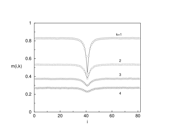
FIG. 8.: Magnetization profile $m(i,k;L)$ at different depths $k$ in films with $L=40$ layers and one additional line of spins on the surface. The simulation was done for $81\times 80$ spins in each layer, couplings $J_{s}=2J_{b}$, $J_{a}=J_{n}=J_{b}$ and temperature $T=0.96T_{c}$. The magnetization in the additional line itself is $m_{l}\approx 0.218$.

B Step

Finally, we briefly report our findings for the critical properties of the step magnetization. A straight step is introduced (actually two steps, to allow for periodic boundary conditions) by adding half a layer of magnetic adatoms to the surface of the magnetic film [14], see Fig. 1(d). We discrimate two couplings, $J_{s}$ if both neighbouring spins are surface spins, and $J_{b}$ otherwise. We consider the line magnetization of the spins at the step edge, $m_{se}$, vanishing on approach to the transition as $m_{se}\propto t^{\beta_{se}}$.

For $J_{s}=J_{b}$, i.e. at the ordinary transition, one obtains $\beta_{se}\approx 0.80$ in semi–infinite Ising models, $L\rightarrow\infty$, i.e. the same value as for the critical exponent of the surface magnetization, as had been shown in a previous Monte Carlo study on thick Ising films with a step [14], in agreement with analytical considerations [26]. However, in thin films, the critical behaviour is quite different. In the simulations, for a single layer $L=1$ plus half a layer, we find a critical exponent close to 1/2 (its concrete value depends rather sensitively on a very accurate determination of $T_{c}$), i.e. a value close to that of the surface critical exponent $\beta_{1}$ of the two-dimensional Ising model (note also its robustness against randomness in the couplings [27]). This observation can be understood in the following way. One is dealing with a composite system displaying, as the layer size goes to infinity, two distinct phase transitions, one at the critical temperature of the Ising plane, $k_{B}T_{c}(L=1)/J_{s}=2.269...$, and one at the critical temperature of the double layer, $k_{B}T_{c}(L=2)/J_{s}\approx 3.2$. Related composite Ising models have been investigated before [28, 29, 30], showing that on approach to the upper critical temperature, where half of the system is disordered, the critical behaviour of the magnetization at the interface (i.e., here, at the step) is governed by the surface critical exponent. The same scenario is expected to hold for finite films with $T_{c}(L+1)>T_{c}(L)$. However, the temperature region where this behaviour can be observed, will become smaller and smaller as $L$ increases.

At the surface transition, the same considerations are believed to be valid. Indeed, in the case $J_{s}=2J_{b}$, we found $\beta_{se}$ to be quite close to 1/2 for a single layer, $L=1$, plus half a layer. For trivial reasons, $\beta_{se}(L=1)=1/2$ holds for $J_{s}\gg J_{b}$, when the bottom layer and the extra half layer decouple with the step edge being the surface of a two–dimensional Ising model. In the thermodynamic limit, where $T_{c}(L+1)=T_{c}(L)$, so that the above decoupling considerations do not apply, we estimated from MC data for films with up to 40 layers, a value of $\beta_{se}=0.33\pm 0.02$. Presumably, in that limit, $\beta_{se}$ is non–universal at the surface transition, depending on the ratio $J_{s}/J_{b}$.

IV Summary

Using density-matrix renormalization group and Monte Carlo techniques, we studied critical properties of magnetic Ising films with various surface defects.

In particular, the effect of the local couplings at one or two additional lines of magnetic adatoms on the surface as well as at straight steps of monoatomic height has been investigated, especially in the limiting cases of films consisting of merely one layer and rather thick films.

In the case of a single layer, $L=1$, with additional lines of magnetic adatoms, the critical exponent of the magnetization at the surface defect is non–universal. The dependence of its value on the local couplings, as compared to that of the perfect two–dimensional situation, follows the trends observed for the exactly soluble two–dimensional Ising model with ladder and chain like bond–defects. The value may be lower or larger than in the perfect situation, 1/8, corresponding to an increase or decrease in the magnetization at the defect line. Adding half a layer of spins, one recovers, at the step, the surface critical exponent, 1/2, of the two–dimensional Ising model.

In the limit $L\rightarrow\infty$, varying the strength of the surface couplings may lead either to a surface or an ordinary phase transition. The change of the critical exponent of the magnetization at the defect has been found to depend only fairly weakly, for both types of transition, on the film thickness $L$ in the case of one additional line of spins. At steps, the critical exponent is argued to be 1/2, for films of finite thickness and both kinds of transition, in agreement with the simulations.

In the paper, we have not only presented the results for the exponents, but also shown various magnetization curves directly, so as to give an impression of the size of the effects. This is meant to encourage further experimental work on such surface structures and their magnetic properties.

- [1] U. Gradmann, J. Magn. Magn. Mater. 100, 481 (1991); P. Poulopoulos and K. Baberschke, J. Phys.–Condens. Mat. 11, 9495 (1999)
- [2] P. Schilbe and K. H. Rieder, Europhys. Lett. 41, 219 (1998).
- [3] Z. Q. Qiu, J. Pearson, and S. D. Bader, Phys. Rev. B 49, 8797 (1994).
- [4] W. Janke and K. Nather, Phys. Rev. B 48, 15807 (1993).
- [5] M. I. Marqués and J. A. Gonzalo, Eur. Phys. J. B 14, 317 (2000).
- [6] F. Iglói, I. Peschel, and L. Turban, Adv. Phys. 42, 683 (1993).
- [7] K. Binder, in Phase Transitions and Critical Phenomena, edited by C. Domb and J. L. Lebowitz (Academic, London, 1983), Vol. 8.
- [8] H. W. Diehl, in Phase Transitions and Critical Phenomena, edited by C. Domb and J. L. Lebowitz (Academic, London, 1986), Vol. 10; H. W. Diehl, Int. J. Mod. Phys. B 11, 3503 (1997).
- [9] H. Dosch, Critical Phenomena at Surfaces and Interfaces, (Springer, Berlin/Heidelberg/New York, 1992).
- [10] T. Kaneyoshi, Introduction to Surface Magnetism, (CRC Press, Boca Raton, Ann Arbor, Boston, 1991).
- [11] J. Shen, R. Skomski, M. Klaua, H. Jenniches, S. Sundar Manoharan, and J. Kirschner, Phys. Rev. B 56, 2340 (1997)
- [12] J. Shen, M. Klaua, P. Ohresser, H. Jenniches, J. Barthel, Ch. V. Mohan, and J. Kirschner, Phys. Rev. B 56, 11134 (1997)
- [13] R. Z. Bariev, Sov. Phys. JETP 50, 613 (1979).
- [14] M. Pleimling and W. Selke, Eur. Phys. J. B 1, 385 (1998).
- [15] F. D. A. Aarão Reis, Phys. Rev. B 58, 394 (1998).
- [16] S. R. White, Phys. Rev. Lett. 69, 2863 (1992), Phys. Rev. B 48, 10345 (1993).
- [17] I. Peschel, X. Wang, M. Kaulke and K. Hallberg (eds.), Density-matrix Renormalization, Lecture Notes in Physics 528 (Springer, Berlin, 1999).
- [18] K. Binder and D. W. Heermann, Monte Carlo Simulations in Statistical Physics (Springer, Berlin/Heidelberg/New York, 1992 ).
- [19] M. Oshikawa and I. Affleck, Phys. Rev. Lett. 77, 2604 (1996); Nucl. Phys. B 495, 533 (1997).
- [20] F. Szalma and F. Iglói, J. Stat. Phys. 95, 759 (1999).
- [21] T. Nishino, J. Phys. Soc. Japan 64, 3598 (1995), see also the article in reference [17].
- [22] M. Pleimling and W. Selke, Phys. Rev. B 59, 65 (1999).
- [23] A. M. Ferrenberg and D. P. Landau, Phys. Rev. B 44, 5081 (1991).
- [24] A. L. Talapov and H. W. J. Blöte, J. Phys. A: Math. Gen. 29, 5727 (1996).
- [25] D. P. Landau and K. Binder, Phys. Rev. B 41, 4633 (1990).
- [26] H. W. Diehl and A. Nüsser, Z. Phys. B. 79, 69 (1990).
- [27] W. Selke, F. Szalma, P. Lajko, and F. Iglói, J. Stat. Phys. 89, 1079 (1997).
- [28] R. Z. Bariev, O. A. Malov, and N. A. Barieva, Physica A 169, 281 (1990).
- [29] B. Berche and L. Turban, J. Phys. A 24, 345 (1991).
- [30] F. Iglói and J. O. Indekeu, Phys. Rev. B. 41, 6836 (1990).