Supersymmetric Hubbard operators

Abstract

We develop a supersymmetric representation of the Hubbard operator which unifies the slave boson and slave fermion representations into a single $U(1)\times SU(1|1)$ gauge theory, a group with larger symmetry than the product of two $U(1)$ gauge groups. These representations of the Hubbard operator can be used to incorporate strong Hund’s interactions in multi-electron atoms as a constraint. We show how this method can be combined with the $SP(N)$ group to yield a locally supersymmetric large-N formulation of the $t-J$ model.

One of the fascinating aspects of strongly correlated materials is their propensity to develop novel metallic phases in situations where local moments interact strongly with mobile electrons. Examples of such situations include metals near a metal insulator transition, [1] metals at an anti-ferromagnetic quantum critical point[2] and anti-ferromagnetic heavy fermion superconductors.[3] These discoveries challenge our understanding of how spin and charge interact at the brink of magnetism.

Theoretical approaches to these problems are hindered by the difficulty of capturing the profound transformation in spin correlations that develops at the boundary between antiferromagnetism and paramagnetism. Usually we model these features by representing the spin as a boson in a magnetic phase,[4] or as a fermion in a paramagnetic phase,[5] but by making this choice, the character of spin and charge excitations which appear in an approximate field theory is restricted and lacks the flexibility to describe the co-existence of strong magnetic correlations within a paramagnetic phase.

These considerations have motivated the development of new methods to describe the spin and charge excitations of a strongly correlated material which avoid making the choice between a bosonic or fermionic spin.[6, 7, 8, 9] This paper attempts to stimulate further progress in this direction by introducing a supersymmetric representation of Hubbard operators.[10] The method used here is an extension of the supersymmetric spin representation introduced by Coleman, Pépin and Tsvelik[11, 12] (CPT). Remarkably, the supersymmetry in the CPT spin representation survives the introduction of charge degrees of freedom, opening the method to a wider range of models.

Hubbard operators[10] provide a way to describe atoms in which Coulomb repulsion prevents double-occupancy of a given orbital. Suppose $|a\rangle\in\{|0\rangle,|\sigma\rangle\}$ describes a set of atomic states involving a charged “hole” $|0\rangle$ or a neutral spin state $|\sigma\rangle$ with spin component $\sigma\in\{1\dots N\}$ which for generality can have one of $N$ possible values. The Hubbard operators are written

$$X_{{a}{b}}=|{a}\rangle\langle{b}|$$ (1)

where ${a},{b}\in\{0,N\}$, represent an atomic state with $N$ possible spin configurations. The operators $X_{\sigma\sigma^{\prime}}$ are bosonic spin operators whereas the $X_{\sigma 0}$ and $X_{0\sigma}$ are fermionic operators that respectively create and annihilate a single electron. The spin operators ${X}_{\sigma\sigma^{\prime}}$ are the generators of the group $SU(N)$. The additional operators expand the group to a supergroup $SU(N|1)$[13] that describes the physical spin and charge degrees of freedom of the atom. These operators satisfy a graded Lie algebra

$$[X_{{a}{b}},X_{{c}{d}}]_{\pm}=\delta_{{b}{c}}X_{{a}{d}}\pm\delta_{{a}{d}}X_{{c}{b}}.$$ (2)

where the plus sign is only used for fermionic operators. The absence of a Wick’s theorem for these operators is normally overcome by factorizing the fermionic Hubbard operators as a product of canonical creation and annihilation operators. This can be done by representing the empty state by a “slave boson” and the spin by a fermion [5] or alternatively, by representing the empty state as a “slave fermion” and the spin by a Schwinger boson.[14]

We now generalize this approach, introducing

$$F_{a} = (f_{1},\dots f_{N},\phi)$$ (3)

$$B_{a} = (b_{1},\dots b_{N},\chi)$$ (4)

where $b_{{\sigma}}$ and $f_{{\sigma}}$ denote a Schwinger boson[4] and Abrikosov pseudo-fermion[17] respectively, while $\phi$ and $\chi$ are slave bosons[5] and fermions[14] respectively. In terms of these operators, the supersymmetric representation of the Hubbard operators is written

$${X}_{{a}{b}}=B_{{a}}^{\dagger}B_{b}+F_{{a}}^{\dagger}F_{b},$$ (5)

Written out explicitly, this is

$$X_{\sigma\sigma^{\prime}} = b^{\dagger}_{\sigma}b_{\sigma^{\prime}}+f^{\dagger}_{\sigma}f_{\sigma^{\prime}}$$ (6)

$$X_{\sigma 0} = b^{\dagger}_{\sigma}\chi+f^{\dagger}_{\sigma}\phi,\qquad X_{0\sigma}=\chi^{\dagger}b_{\sigma}+\phi^{\dagger}f_{\sigma}$$ (7)

$$X_{00} = \chi^{\dagger}\chi+\phi^{\dagger}\phi$$ (8)

By summing the slave fermion and slave boson representations we are guaranteed that the representation satisfies the correct commutation algebra. The novelty of our approach lies in the two unique constraints which make the representation irreducible, which we show to be

$$Q=n_{{b}}+n_{{\phi}}+n_{{f}}+n_{{\chi}},$$ (9)

the total number of particles and

$$Y=n_{{\phi}}+n_{{f}}-(n_{{b}}+n_{{\chi}})+\frac{1}{Q}[\theta,\theta^{\dagger}],$$ (10)

the “asymmetry” of the representation, where $\theta=\sum_{\sigma}{b}_{\sigma}^{\dagger}{f}_{\sigma}-{\chi}^{\dagger}{\phi}$ and its conjugate $\theta^{\dagger}$ are fermionic operators which satisfy the algebra $\{\theta,\theta^{\dagger}\}=Q$. The $\theta$ operators interconvert bosons and fermions.

$\displaystyle b_{\sigma}{\mathop{\hbox{\ooalign{\raise 2.0pt\hbox{$\relbar\joinrel\relbar\joinrel\rightharpoonup$}\crcr{\hbox{$\leftharpoondown\joinrel\relbar\joinrel\relbar$}}}}}^{\displaystyle\theta^{\dagger}}_{\displaystyle\theta}}f_{\sigma},\qquad-\chi{\mathop{\hbox{\ooalign{\raise 2.0pt\hbox{$\relbar\joinrel\relbar\joinrel\rightharpoonup$}\crcr{\hbox{$\leftharpoondown\joinrel\relbar\joinrel\relbar$}}}}}^{\displaystyle\theta^{\dagger}}_{\displaystyle\theta}}\phi\qquad$

The special feature of this representation is that $\theta$ and $\theta^{\dagger}$ commute with the constraints $[\theta^{(\dagger)},Q]=[\theta^{(\dagger)},{Y}]=0$, the bosonic Hubbard operators

$\displaystyle[\theta^{(\dagger)},X_{\sigma\sigma^{\prime}}]=[\theta^{(\dagger)},X_{00}]=0,$

and they also anti-commute with the fermionic Hubbard operators

$\displaystyle\{\theta^{(\dagger)},X_{\sigma 0}\}=\{\theta^{(\dagger)},X_{{0\sigma}}\}=0,$

so that there is a local supersymmetry which underlies the constraint. The operators $Q$, $\theta$ and $\theta^{\dagger}$ are the generators of the simplest supergroup $SU(1|1)$[13]; the operator $Y$ generates an additional $U(1)$ symmetry. Remarkably, by combining the slave boson and slave fermion representations, the abelian gauge groups of the starting representation “fuse” into a supergroup with greater symmetry $U_{SB}(1)\times U_{SF}(1)\rightarrow U(1)\times SU(1|1).$ If we introduce the operator $\hat{A}=[\bar{\eta}\theta-\theta^{\dagger}\eta]$, where $\eta$ and $\bar{\eta}$ are Grassman numbers, then under an $SU(1|1)$ rotation, the fields $\psi_{{a}}=\textstyle\left(\matrix{\textstyle B_{{a}}\cr F_{{a}}}\right)$ transform as

$$\psi_{{a}}\rightarrow e^{A}\psi_{{a}}e^{-A}=\psi_{{a}}+[A,\psi_{{a}}]+\frac{1}{2}[A,[A,\psi_{{a}}]]$$ (11)

where the Grassman coefficients truncate the expansion at second-order. Expanding this expression gives $\psi_{a}\rightarrow h\psi_{a}$, $\psi^{\dagger}_{b}\rightarrow\psi^{\dagger}_{b}h^{\dagger}$ where

$\displaystyle h=\left(\matrix{\sqrt{1-\bar{\eta}\eta}&-\bar{\eta}\cr\eta&\sqrt{1-\eta\bar{\eta}}}\right).$

is an $SU(1|1)$ matrix, satisfying $h^{\dagger}h=1$ The ${X}$-operators (5) can be written as ${X}_{{a}{b}}=\psi_{a}^{\dagger}\psi_{b}$. Under the action of the $SU(1|1)$ group, $X_{ab}\rightarrow\psi^{\dagger}_{a}h^{\dagger}h\psi_{b}=X_{ab}$, explicity demonstrating the local gauge invariance.

To guarantee that the Hubbard operator representation is irreducible, we need to set the values of the linear and quadratic Casimirs of the $SU(N|1)$ group. Under the $SU(N|1)$ group, the spinors $B$ and $F$ transform according to $B\rightarrow B\tilde{U}$, $F\rightarrow F\tilde{U}$,[15] where $\tilde{U}\equiv U^{st}$ denotes the supertranspose of the unitary $SU(N|1)$ matrix, $U\$ [16].The Hubbard operators $X_{ab}=B^{\dagger}_{a}B_{b}+F^{\dagger}_{a}F_{a}$ thus transform according to $X_{ab}\rightarrow(\tilde{U}^{\dagger}X\tilde{U})_{ab}$. Since $U^{\dagger}U=1$, it follows that $U^{st}(U^{\dagger})^{st}=1$. However, the supertranspose and hermitian conjugate do not commute and are related by $(U^{\dagger})^{st}=g(U^{st})^{\dagger}g$, where $g=Diag[1\dots 1,-1]$ is the invariant metric tensor of $SU(N|1)$. Thus the $\tilde{U}$ are not unitary, but satisfy $\tilde{U}g\tilde{U}^{\dagger}=g$. Using the property that $\hbox{Tr}[AB]=\hbox{Tr}[BgAg]$, it follows that

$$C^{(1)}=\hbox{Tr}[{X}],\qquad C^{(2)}=\hbox{Tr}[XgX],$$ (12)

are invariant under the transformation $X\rightarrow\tilde{U}^{\dagger}X\tilde{U}$. These are the linear and quadratic Casimirs of the $SU(N|1)$ group. Inserting (6) into (12), we find that $C^{(1)}=Q$, while the quadratic Casimir is

$$C^{(2)}=X_{\sigma\sigma^{\prime}}X_{\sigma^{\prime}\sigma}-X_{\sigma 0}X_{0\sigma}+X_{0\sigma^{\prime}}X_{\sigma^{\prime}0}-X_{00}^{2}$$ (13)

where summation over $\sigma,\sigma^{\prime}\in\{1,N\}$ is implied. When we expand the Casimir in terms of the canonical creation and annihilation operators, we find that

$$C^{(2)}=\hat{Q}(N-1-{\hat{Y}}),$$ (14)

with $Q$ and $Y$ as given in (9) and (10 ). So by defining ${Y}$ and $Q$, we uniquely set the representation.

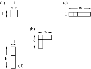
FIG. 1.: (a) Fundamental representation $(Q,Y)=(1,0)$, (b) L-shaped Young tableau corresponding to the spin representation generated by supersymmetric Hubbard operators. The asymmetry ${Y}=h-w$ and $Q$ is the number of boxes, (c) Young tableau for fully symmetric representation corresponding to Slave fermion limit (d) Fully antisymmetric, slave boson limit.

Each conserved value of $(Q,Y)$ describes an irreducible representation of the $SU(N|1)$ group; the fundamental representation, $(Q,Y)=(1,0)$ corresponds to an atomic orbital with no double occupancy (Fig. 1(a)). More general representations involve spin wavefunctions with symmetric and antisymmetric correlations, denoted by an “$L-$ shaped” Young tableau[18] with $Q$ boxes, where ${Y}=h-w$ is the difference between the height and width (Fig. 1 (b-d)). These representations describe the physics of multi-electron atoms where the spins are Hund’s coupled, and in this way strong Hund’s couplings can be incorporated into an infinite $U$ Anderson model using the constraints (9) and (10 ). As an example, the material $LiV_{2}O_{4}$ develops a paramagnetic heavy fermion ground-state[19] in which vanadium ions form a mixed valence admixture of a $d^{1}(S=1/2)$ and a Hund’s coupled $d^{2}(S=1)$ state. Since the electrons in the $d^{{2}}$ configuration are in a symmetric wavefunction, corresponding to a row-tableau, this situation is described by Hubbard operators in the representation $(Q,Y)=(2,-1)$:

$\displaystyle{e^{-}+\overbrace{\hbox{}\vbox{\vbox{\offinterlineskip\vbox{\hrule height=0.3pt\hbox{\vrule height=8.74669pt,width=0.3pt,depth=2.18663pt\hbox to10.93333pt{\hfil}\vrule height=8.74669pt,width=0.3pt,depth=2.18663pt} \hrule height=0.3pt}\vspace{-\y@linethick} }}}^{\hbox{$d^{1}$}}\rightleftharpoons\overbrace{\hbox{}\vbox{\vbox{\offinterlineskip\vbox{\hrule height=0.3pt\hbox{\vrule height=8.74669pt,width=0.3pt,depth=2.18663pt\hbox to10.93333pt{\hfil}\vrule height=8.74669pt,width=0.3pt,depth=2.18663pt\hbox to10.93333pt{\hfil}\vrule height=8.74669pt,width=0.3pt,depth=2.18663pt} \hrule height=0.3pt}\vspace{-\y@linethick} }}}^{\hbox{$d^{2}$}}}\quad.$

As a second example, consider $UPd_{2}Al_{3}$ in which uranium atoms fluctuate between an $f^{2}$ and an $f^{{3}}$ configuration. Surprisingly, part of the spin magnetically orders, while the remainder forms a singlet superconductor with the conduction electrons.[3] In this case, the f-electrons are spin-orbit coupled, with $j=5/2$, forming an $SU(N)$ multiplet with $N=2j+1=6$. In practice, crystal field effects break this large degeneracy, but a toy model for the physics can be obtained using $SU(N)$ Hubbard operators to describe the charge fluctuations, subject to the constraint $(Q,Y)=(2,1)$. This leads to valence fluctuations involving an $L-$ shaped spin $f^{3}$ spin configuration:

$\displaystyle{e^{-}+\overbrace{\hbox{}\vbox{\vbox{\offinterlineskip\vbox{\hrule height=0.3pt\hbox{\vrule height=8.74669pt,width=0.3pt,depth=2.18663pt\hbox to10.93333pt{\hfil}\vrule height=8.74669pt,width=0.3pt,depth=2.18663pt} \hrule height=0.3pt}\vspace{-\y@linethick} \vbox{\hrule height=0.3pt\hbox{\vrule height=8.74669pt,width=0.3pt,depth=2.18663pt\hbox to10.93333pt{\hfil}\vrule height=8.74669pt,width=0.3pt,depth=2.18663pt} \hrule height=0.3pt}\vspace{-\y@linethick} }}}^{\hbox{$f^{2}$}}\rightleftharpoons\overbrace{\hbox{}\vbox{\vbox{\offinterlineskip\vbox{\hrule height=0.3pt\hbox{\vrule height=8.74669pt,width=0.3pt,depth=2.18663pt\hbox to10.93333pt{\hfil}\vrule height=8.74669pt,width=0.3pt,depth=2.18663pt\hbox to10.93333pt{\hfil}\vrule height=8.74669pt,width=0.3pt,depth=2.18663pt} \hrule height=0.3pt}\vspace{-\y@linethick} \vbox{\hrule height=0.3pt\hbox{\vrule height=8.74669pt,width=0.3pt,depth=2.18663pt\hbox to10.93333pt{\hfil}\vrule height=8.74669pt,width=0.3pt,depth=2.18663pt} \hrule height=0.3pt}\vspace{-\y@linethick} }}}^{\hbox{$f^{3}$}}}\quad.$

In this scheme the vertical leg of the representation can form a singlet with conduction electrons, leaving a single residual spin free to magnetically order.[12]

In many problems we are interested in interacting atoms containing either one, or zero electrons. Physical states corresponding to this situation have $Q=1,Y=0$:

$$\hat{Q}|\psi\rangle=|\psi\rangle,\quad\hat{Y}|\psi\rangle=0.$$ (15)

These conditions do not force the representation into a slave boson, or slave fermion representation. Here, it is useful to note that $\theta$ and $\theta^{\dagger}$ behave as lowering, and raising operators. In fact, because $\{\theta,\theta^{\dagger}\}=Q$,

$\displaystyle\tau_{+}=\frac{1}{\sqrt{Q}}\theta^{\dagger},\quad\tau_{-}=\frac{1}{\sqrt{Q}}\theta,\quad\tau_{z}=[\tau_{+},\tau_{-}]=\frac{1}{{Q}}[\theta^{\dagger},\theta],$

behave as the raising, lowering and z components of a “superspin” operator. If we take the sum and difference of the constraints (9) and (10), we find that for $Q=1$

$$n_{f}+n_{\phi} = \frac{1}{2}(1+\tau_{z}),$$ (16)

$$n_{b}+n_{\chi} = \frac{1}{2}(1-\tau_{z}).$$ (17)

For $\tau_{z}=1$ these equations revert to the constraints for a slave boson representation, when ${\tau_{z}}=-1$, they revert to those of a slave fermion representation, i.e an “up” superspin corresponds to a slave boson state, $\frac{1}{2}(1+\tau_{z})|\psi\rangle=|\psi_{F}\rangle$, a “down” superspin corresponds to a slave-fermion state $\frac{1}{2}(1-\tau_{z})|\psi\rangle=|\psi_{B}\rangle$. In the supersymmetric approach, a partition function of a Hamiltonian $H$, involves tracing over both slave boson and slave fermion representations,

$\displaystyle Z=\sum_{\lambda\in F,B}\langle\psi_{\lambda}|e^{-\beta H}|\psi_{\lambda}\rangle.$

The trace over both subspaces means that the derived path integral has a $U(1)\times SU(1|1)$ symmetry and new dynamical degrees of freedom. In the slave fermion and slave boson schemes, Fermi liquid and magnetic phases are manifested as “Higgs phases” of the $U(1)$ gauge group. [20] The enlarged $U(1)\times SU(1|1)$ gauge group unifies the slave boson and slave fermion schemes, but also extends beyond it to furnish a potentially wider class of Higgs phases. For instance, suppose $H$ is a Hamiltonian, such as the $t-J$ model with both magnetic and paramagnetic phases, then we expect $\langle\tau_{z}\rangle=-1$ in the anti-ferromagnetic (insulating) ground-state and $\langle\tau_{z}\rangle=+1$ in the paramagnetic ground-state, but in addition, there is the possibility of new saddle-points where $\langle\tau_{z}\rangle$ lies between these two extreme values.

We end with a discussion on the formulation of the $t-J$ model as a supersymmetric large-$N$ expansion. To handle anti-ferromagnetic interactions and electron hopping in a large $N$ expansion, we adopt the Read-Sachdev scheme, using Hamiltonians that are globally invariant under the unitary symplectic group $SP(N)$[21]. This group is a subgroup of $SU(N)$ (defined only for even values of $N=2n$), so its generators are a subset of the Hubbard operators. Moreover, the groups $SP(2)$ and $SU(2)$ are equivalent. In $SP(N)$, the spin components are divided into an equal number of “up” and “down” values $\sigma\in(\pm 1,\dots\pm N/2)$; the unitary matrices of SP(N) satisfy the condition $U^{T}\underline{\epsilon}U=\underline{\epsilon}$, where ${\epsilon}_{\sigma\sigma^{\prime}}={\rm sgn}(\sigma)\delta_{\sigma,-\sigma^{\prime}}$. The $SP(N)$ $t-J$ model is written[22]

$$H = -\frac{t}{N}\sum_{(i,j)}[X_{\sigma 0}(i){\rm X}_{0\sigma}(j)+{\rm H.c}]$$ (18)

$$+ \frac{J}{N}\sum_{i,j}\epsilon_{\sigma\sigma^{\prime}}\epsilon_{\eta\eta^{\prime}}X_{\sigma\eta^{\prime}}(i)X_{\sigma^{\prime}\eta}(j)-\mu\sum_{j}{\cal N}_{j}$$ (19)

where ${\cal N}_{j}=\sum_{\sigma}X_{\sigma\sigma}(j)$ is the number of particles. In the supersymmetric representation, this model becomes $H+\sum_{j}K_{j}$

$$H = -\frac{t}{N}\sum_{(i,j)}[(f^{\dagger}_{i\sigma}\phi_{i}+b^{\dagger}_{i\sigma}\chi_{i})(\phi^{\dagger}_{j}f_{j\sigma}+\chi^{\dagger}_{j}b_{j\sigma})+{\rm H.c.}]$$ (20)

$$- \frac{J}{N}\sum_{(i,j)}{\rm Tr}[\Lambda^{\dagger}_{ij}\Lambda_{ij}]-\mu\sum_{j}{\cal N}_{j},$$ (21)

where $K_{j}=\lambda_{j}(\hat{Q}_{j}-Q_{0})+\zeta_{j}(Y_{j}-Y_{0})$ describes the constraints at site $j$, ${\cal N}_{j}=n_{f}(j)+n_{b}(j)$ and

$\displaystyle\Lambda_{ij}={\epsilon}_{\sigma\sigma^{\prime}}\left[\matrix{f_{i\sigma}f_{j\sigma^{\prime}}&f_{i\sigma}b_{j\sigma^{\prime}}\cr b_{i\sigma}f_{j\sigma^{\prime}}&b_{i\sigma}b_{j\sigma^{\prime}}}\right]$

describes the singlet valence bonds between site $i$ and site $j$. This Hamiltonian is invariant under the global $SP(N)$ transformation and the local $U(1)\times SU(1|1)$ gauge group. The family of models with $(Q_{0},Y_{0})=(N/2,0)$, ($N$ even) are of particular interest. Two points deserve special mention:

i) In a path integral treatment, by carrying out a local gauge transformation $\psi_{j}\rightarrow g_{i}(\tau)\psi_{i}$ and integrating over $g_{j}$, one obtains a supersymmetric Lagrangian[11], ${\cal L}={\cal L}_{susy}+H$, where

$\displaystyle{\cal L}_{susy}=\sum_{j,a}\psi_{ja}^{\dagger}\biggl{[}\partial_{\tau}-\lambda_{j}+\zeta_{j}\tau_{3}\biggr{]}\psi_{ja}-\frac{1}{Q_{o}}\theta_{j}^{\dagger}(\partial_{\tau}+2\zeta_{j})\theta_{j}.$

This is the starting point for the study of the various Higgs phases of the model. In each of these phases, one of the fermi fields is absorbed into the fluctuations of the gauge field. For instance, in paramagnetic phases the slave boson condenses and by fixing

$\displaystyle\psi_{j}=g_{j}\left(\matrix{b^{\prime}_{j\sigma_{1}}&\dots b^{\prime}_{j\sigma_{N}}&0\cr f^{\prime}_{j\sigma_{1}}&\dots f^{\prime}_{j\sigma_{N}}&r_{j}}\right),$

the slave fermions $\chi_{j}$ are absorbed into the gauge field. Similary, the Schwinger boson field $b_{\sigma}$ condenses in an ordered anti-ferromagnetic phase, absorbing a component of the $f_{\sigma}$ fields. More complex Higgs phases, in which fermi fields of the bond variables are absorbed into plaquet fermions also become possible.

ii) The Lagrange multiplier $\zeta_{j}$ which imposes the constraint on $Y_{j}$ gives rise to a self-consistently determined spin interaction $H_{I}=-\frac{2\zeta_{j}}{Q}\theta_{j}^{\dagger}\theta_{j}$, resembling recent approaches to the Hubbard model in which spin interactions self-consistently renormalize to enforce local constraints[23]. The Gaussian fluctuations of the $\theta$ fields associated with this spin interaction play a crucial role in enforcing the constraints between slave boson and slave fermion fields, and non-trivial results depend on the inclusion of these fluctuations in the effective action.

In conclusion, we have presented a supersymmetric representation of Hubbard operators in which both the operators and the constraints are invariant under the action of the supergroup $U(1)\times SU(1|1)$. This approach avoids the need to choose between a fermionic, or bosonic representation for spins. The underlying $U(1)\times SU(1|1)$ gauge group is larger than the simple product of two $U(1)$ gauge groups. Broken symmetry saddle points of this enlarged group provide the opportunity to study the interplay between magnetism and paramagnetism.

This work was supported in part by the National Science Foundation under grants DMR 9983156 (PC and JH) and PHY 99-07947 (PC and CP) and research funds from the EPSRC, UK (CP). PC and CP would like to thank the Isaac Newton Institute and the Institute for Theoretical Physics, Santa Barbara, where part of this work was carried out.

REFERENCES

[1]See
J. Orenstein and A. J. Millis, Science 288, 468, (2000);
P. W. Anderson, Science 288, 480, (2000) and references therein.
[2]N. D. Mathur et al., Nature, 394, 39 (1998).
[3]R. Feyerherm et al., Phys Rev. Lett. 73, 1849 (1994).
[4]D. P. Arovas and A. Auerbach,
Phys. Rev B 38, 316-211, 1988.
[5]P. Coleman, Phys. Rev. B 29, 3035
1984); A. J. Millis and P. A. Lee, Physical
Review B-Condensed Matter, 35, 3394 (1987).
[6]J. Gan , P. Coleman, N. Andrei Phys. Rev. Lett. 68, 3476, (1992); J. Gan and P. Coleman, Physica B, 171, 3 (1991).
[7]C. Pépin and M. Lavagna , Phys. Rev. B, 59, no.19,12180 (1999);Z. Phys. B 103, 259 (1997).
[8]O. Parcollet and A. Georges, Phys. Rev. Lett. 79, 4665 (1997).
[9]T. K. Ng and C. H. Cheng, Phys. Rev. B59, R6616
(1999).
[10]J. Hubbard, Proc. Royal Society A 277, 237 (1964).
[11] P. Coleman, C. Pépin, A. M. Tsvelik, Phys. Rev. B 62,
3852-3868 (2000).
[12] P. Coleman, C. Pépin and A. M. Tsvelik, Nuclear Physics
B586, pp. 641-667 (2000).
[13]I. Bars,
Physica D, 15D, 42 (1985).
[14]C. Jayaprakash et. al., Phys. Rev. B40,
2610 (1989); D. Yoshioka, J. Phys. Soc. Japan, 58, 1516 (1989);
C.L. Kane et.al., Phys. Rev. B41, 2653 (1990).
[15]The transpose matrices must be used, because both and
are column supervectors.
[16]
See, for example J. F. Cornwall, “Group Theory in Physics”, Vol 3, p18,
Academic Press, London (1989).
[17]A. A. Abrikosov, Physics 2, 5 (1965).
[18]For a reference on Young tableaux, see e.g.
M. Hammermesh, “Group Theory and its Application to Physical Problems”,
pp 198, Addison Wesley, (1962).
[19]C. Urano et al, Phys. Rev. Lett. 85 ,1052, (2000).
[20]In these phases,
Elitzur’s theorem assures that
the local gauge group is not
actually broken, but the slave fields at each site develop
power-law correlations in time and may
in this sense be said to have developed
long-range order in time.
[21]N. Read and Subir Sachdev, Phys. Rev. Lett,
66, 1773 (1991); Subir Sachdev and Ziquiang Wang, Phys Rev B
43, 10229, (1991).
[22] Mathias Vojta, Ying Zhang and Subir Sachdev,
cond-mat 0003163.
[23]Y. Vilk and A. M. Tremblay, J Phys. France, I7,
1339 (1997).