On the Effects of a Bulk Perturbation on the Ground State of 3D Ising Spin Glasses

Abstract

We compute and analyze couples of ground states of $3D$ spin glasses before and after applying a volume perturbation which adds to the Hamiltonian a repulsion from the true ground state. The physical picture based on Replica Symmetry Breaking is in excellent agreement with the observed behavior.

Studying the scaling behavior of ground states (GS) of disordered systems [1] turns out to be a powerful tool. Here by using a powerful technique based on a bulk modification of the Hamiltonian [2, 3] we are able to give strong numerical evidence of a Replica Symmetry Breaking like behavior of $3D$ spin glasses. With this study we believe we vastly enlarge the scope of [4], where we were changing the boundary conditions to analyze the changes induced in the GS microscopic structure. The open debate is about the role of the exact (Replica Symmetry Breaking, RSB) solution of the Mean Field spin glass model, where field theory is exact by definition [5], in describing finite dimensional spin glasses: the validity of a possible phenomenological description, the (more or less modified) droplet picture [6], should probably be taken as an alternative possibility. The RSB picture is characterized by the presence of states (for the terminology we refer to [3]) that are locally different one from the other.

In this respect equilibrium Monte Carlo simulations are useful [3], but since it is impossible to thermalize large, low $T$ systems, if one is not far enough from $T_{c}$ there is the remote possibility [7] that the asymptotic physical picture could be disguised because of crossover effects (this criticism does not apply to the off-equilibrium simulations [8], and very low $T$ recent simulations [9] also claim to disprove it). The remarkable achievement of the work of [1] has been to realize that one can compute GS for systems of size comparable to the one of finite $T$ numerical simulations. The first series of papers [1, 4] has been computing couples of GS with periodic boundary conditions (PBC) and with anti-periodic boundary conditions (APBC). A different method, based on the use of a bulk perturbation [2] has been first used by Palassini and Young to detect the inconsistency of a (even modified) droplet picture: large scale excitations with a finite energy cost (first discussed in [10]) are clearly detected by this approach. In the replica approach we expect that these large scale excitations correspond to the simultaneous reverse of a large non-compact block of spins: the surface to volume ratio of the set of the flipped spins should asymptotically go to a non-zero value. In previous studies [10, 2] this surface to volume ratio was investigated: it was found that it was slowly decreasing with $L$ and its behavior was compatible with a small negative power of $L$.

We use here the same method to make stronger the evidence of the existence of these large scale excitations, and we present a detailed quantitative study of their properties. We show that they behave in agreement with RSB, and that the surface to volume ratio extrapolates to a non-zero value in the limit $L\to\infty$.

We work in three spatial dimensions ($D=3$) on simple cubic lattices of linear size $L$, containing $N=L^{3}$ spins with PBC (we have taken $L=4$, $6$, $8$, $10$, $12$, $14$). We consider quenched random couplings $J$ extracted from a Gaussian probability distribution with zero expectation value and unit variance. We study the behavior of the GS after changing the Hamiltonian to include a term which repels from the true GS. The Hamiltonian of the first system is

$$H_{0}(\{\sigma\})\equiv-\sum_{i,\mu}\sigma(i)J(i,\mu)\sigma(i+\hat{\mu})\ ,$$

where the sum is over the $N$ sites $i$ and the $D$ directions $\mu$ ($\hat{\mu}$ is the versor in the $\mu$ direction). The Hamiltonian of the second system is

$$H_{1}(\{\tau\})\equiv H_{0}(\{\tau\})-\frac{\epsilon}{ND}\sum_{i,\mu}\sigma_{0}(i)\sigma_{0}(i+\hat{\mu})\tau(i)\tau(i+\hat{\mu})\ ,$$

where the $\sigma_{0}(i)$ are the spins in the GS of $H_{0}$. Let $\tau_{0}(i)$ be the spins in the GS of $H_{1}$: we are interested in studying the differences among $\sigma_{0}$ and $\tau_{0}$ when $N$ goes to infinity at fixed $\epsilon$ (in this limit the perturbation is of order 1, while the total Hamiltonian is of order $N$). At this end we define the local site overlap on site $i$ as $q(i)\equiv\sigma_{0}(i)\ \tau_{0}(i)$, and the local link overlap is defined among nearest neighbor sites (or equivalently on links) as $q_{l}(i,\mu)\equiv q(i)\ q(i+\mu)$. If two spin configurations differ by a global spin flip their link overlap is identically equal to $+1$ (while their overlap is equal to $-1$). We also define the average over the system sites and links of the previous quantities: $q\equiv N^{-1}\sum_{i}q(i)$, $q_{l}\equiv(DN)^{-1}\sum_{i,\mu}q_{l}(i,\mu)$. With these definitions we have that $H_{1}(\{\tau\})=H_{0}(\{\tau\})-\epsilon q_{l}$. We are considering this type of perturbation because the quantity $q_{l}$ is sensitive only to local changes of the configuration, i.e. it is different from 1 only on the interface among the clusters of flipped and non-flipped spins.

The main effect of the perturbation is to generate excited states. It is reasonable to assume that for $L\to\infty$ the value of the observables computed for fixed value of the site overlap are weakly dependent on the value of $\epsilon$. This is also suggested by the results of [2], and will be discussed in more details in [11]. For this reason we will consider the link overlap (and also other quantities) as a function of the (square) site overlap, i.e. $q_{l}(q^{2})$. This quantity is defined as the average of the link overlap over those systems for which the square site overlaps of the two ground state is $q^{2}$. We will indicate the link overlap summed over all the systems by $\overline{q}_{l}\equiv\int dq^{2}q_{l}(q^{2})P(q^{2})$, where $P(q^{2})$ is the probability distribution of $q^{2}$. We have computed $10^{4}$ GS at $L=4$ and $6$, $2000$ at $L=8$, $1500$ at $L=10$, $500$ at $L=12$ and $14$, with $\epsilon=4\sqrt{6}$, using a genetic algorithm which will be described in [11].

Given the importance of the issue, we start by discussing the dependence of $q_{l}(q^{2})$ over $q$ and $L$. If we plot $q_{l}(q^{2})$ versus $q^{2}$, we notice that $q_{l}(q^{2})$ and $q^{2}$ are very strongly correlated. In order to clarify this effect we define the quantity (for all systems such that $q\neq 1$) $R_{L}(q^{2})\equiv(1-q_{l}(q^{2}))/(1-q^{2})$. For fixed $L$ $R_{L}(q^{2})$ is nearly $q^{2}$ independent in a large region where $q$ is not too large (only close to $q=1$ the dependence becomes slightly more noticeable). The $q^{2}$ dependence of $R(q)$ in this large $q$ region becomes milder with increasing $L$. We fit $R_{L}(q^{2})$ to the form $A(L)+B(L)\ q^{2}$ using the data in the range $q^{2}\in(0,0.3)$: the fits are very good, and the extrapolations are all very smooth. $B(L)$ is in all cases a few percent of $A(L)$. In fig. 1 the upper points are for $A(L)\equiv R_{L}(0)=1-q_{l}(0)$ versus $L^{-1}$. Both a linear fit (which extrapolates to a non zero value) and a power fit to the form $CL^{-\alpha}$, where $\alpha$ turns out to be $0.44$, follow the data in a qualitative way, but they are unacceptable because they lead to a very high value of $\chi^{2}$ (i.e. to a normalized $\chi^{2}=O(20)$). In fig. 1 we plot a second order polynomial fit that is very good (it has a normalized $\chi^{2}\simeq 0.6$) and leads to a value of $A(L=\infty)=0.30\pm 0.01$. We also plot a fit to the form $A(L)=a+bL^{-\lambda}$, that is also good (it has a normalized $\chi^{2}=0.3$) and leads to a value of of $A(L=\infty)=0.24\pm 0.01$ and $\lambda=0.72\pm 0.02$. The difference with the $0.30$ obtained by the polynomial fit gives an idea of the size of the systematic error over the extrapolation.

The values extrapolated to $L=\infty$ are an estimate of $1-q_{l}(0)$, and they have to be compared with the value $0.245\pm 0.015$ that we have estimated in [4]: the agreement is good, even if here the systematic error is large. We can conclude that there is evidence that $1-q_{l}(0)$ does not extrapolate to zero in the infinite volume limit and the dependence of $q_{l}(q^{2})$ is well approximated (for $q^{2}$ not too close to $1$) by the form $q_{l}(q^{2})=1-A(1-q^{2})$. The previous formula holds in the infinite range SK model, with $A=1$. The fact that in $3D$ we find a low value ($A\simeq 0.3$) suggests that $A$ goes to zero when one approaches the lower critical dimension.

The lower points and curves of fig. 1 are for the expectation value of the link overlap $\overline{q}_{l}$, averaged over all $q^{2}$ values. The curves are again a polynomial and a power law best fits, that here extrapolate to a lower value ($0.07\pm 0.04$ for the power law and $0.155\pm 0.015$ for the polynomial fit). The error is larger than in $A(L)$ (of a factor close to $2$) but apart from a shift (since $\overline{q}_{l}\neq q_{l}(0)$) the two curves are similar.

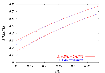
FIG. 1.: The value of $A(L)$ (upper points) and of $\overline{q}_{l}$ as a function of $L^{-1}$. The curves are for a power fit and a polynomial fit.

Let us stress that $A(L)$ is important also since $q_{l}(q^{2})$ is not expected to depend on $\epsilon$ when $L\to\infty$. The $\epsilon$-perturbation allows to explore low energy states with an energy gap of order $1$. The function $P(q^{2})$ changes with $\epsilon$ [12] and consequently also the value $\overline{q_{l}}$ changes: still the functional relation that relates $q_{l}$ to $q^{2}$ is unchanged.

It is also interesting to look at the variance squared of $R_{L}(q^{2})$, i.e. to $\sigma_{(R)L}^{2}(q^{2})\equiv\langle R_{L}^{2}(q^{2})\rangle-\langle R_{L}(q^{2})\rangle^{2}$. We proceed as for the the best fit of $R_{L}(q^{2})$. First we fit $\sigma_{(R)L}^{2}(q^{2})$ to the form $A_{W}(L)+B_{W}(L)\ q^{2}$, using the data with $q^{2}\leq 0.3$: the extrapolations are very good. Also here for a given value of $L$ we find that $\sigma_{(R)L}^{2}(q^{2})$ is nearly $q^{2}$ independent apart from the region close to $q^{2}=1$. Also the $q^{2}$ dependence of $\sigma_{(R)L}^{2}(q^{2})$ in this region becomes weaker mild with increasing $L$.

We plot $A_{W}(L)$ versus $1/L$ in fig. 2. Together with the data we show a best fit to the form $A_{W}(L)\simeq C\ L^{-\delta}$, that has a low $\chi^{2}$, and $\delta=1.35\pm 0.03$. The fact that a fit to a zero asymptotic value is very good shows that $q_{l}$ as a function of $q$ does not fluctuate as $L\to\infty$: this is the same situation that we find in the mean field RSB theory, with a more complex dependence of $q_{l}(q^{2})$ over $q^{2}$. The asymptotically vanishing value of $A_{W}(L)$ explains why the errors on $q_{l}(q^{2})$ are smaller that those on $\overline{q_{l}}$.

We discuss next the overlap-overlap correlation functions. The difference among a droplet and a RSB scenario becomes very clear if we consider the overlap-overlap correlation function at fixed value of $q^{2}$ in a system of side $L$, i.e. the correlation function obtained by selecting those systems which have a ground state with a fixed value of the mutual overlap:

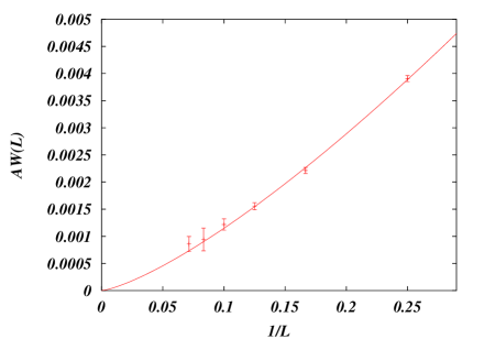
FIG. 2.: The value of $A_{W}(L)$ as function of $L^{-1}$. The curve is a power fit to a zero asymptotic value.

$$C(x,L|q^{2})\equiv\langle q(x)q(0)\rangle_{(q^{2})}\ .$$

In the RSB case we expect that for large $L$ and fixed $x$ $C(x,L|q^{2})\to G(x|q^{2})+q^{2}$, where the function $G(x|q^{2})$ depends on $q^{2}$ and for large $x$ should behave as $G(x|q^{2})\propto x^{-\phi(q^{2})}$. $\phi(q^{2})$ may depend on $q^{2}$, although there are indications that it takes at most only two different values, one at $q=0$ and one at $q\neq 0$ [13]. In the region where $x$ and $L$ are large we expect that

$$C(x,L|q^{2})\approx g(r|q^{2})(\frac{1}{x}+\frac{1}{L-x})^{\phi(q^{2})}+q^{2}\ ,$$ (1)

where $r\equiv xL^{-1}$. We have used the factor $(\frac{1}{x}+\frac{1}{L-x})$ instead of the simpler $\frac{1}{x}$ in order to implement the symmetry implied by the presence of PBC.

The situation described by a droplet picture is different: in this case, for large $L$ and fixed $x$, $C(x,L|q^{2})\to 1$. One can argue that in the droplet model one should have $\phi(q^{2})=0$ and $g(0|q^{2})+q^{2}\simeq 1$, i.e $C(x,L|q^{2})\approx D(xL^{-1}|q^{2})$ with $D(0|q^{2})=1$.

We will discuss our results for small values of $q$: we consider the $q$ range $q\leq q_{max}=0.1$. The results are not very sensitive to the exact position of the $q_{max}$ cut (of course if $q_{max}$ is too small the statistics fades). In fig. 3 we present our data for $g(r)$ as a function of $w\equiv r(1-r)$ for $\phi=0.4$ (we prefer to plot $g$ versus $w$ since because of the PBC both $g$ and $w$ are left invariant when $r$ goes in $1-r$). The value of $q^{2}$ we use to subtract the disconnected part is the average of $q^{2}$ in the interval $q\leq q_{max}$. We have selected $\phi$ such to optimize the quality of the scaling behavior. The line is for the best fit to a second order polynomial.

The scaling is very good, and the estimate of $\phi\simeq 0.4$ reliable. A droplet-like scaling is excluded by our data. We notice that $C(x,L|0)|_{x=1}=q_{l}(0)$ and the scaling form (1) accounts for the $L$-dependence of $q_{l}(0)$. If we assume that (1) is exact also for $x=1$ (a too strong assumption) we get that $C(1,\infty|0)=g(0|0)$. Using the quadratic fit in fig. 3 to extrapolate the data at $r=0$ we get in the infinite volume limit $1-q_{l}(0)=.33\pm.02$, which is in reasonable agreement with the previous estimates, given the crudeness of the approximation.

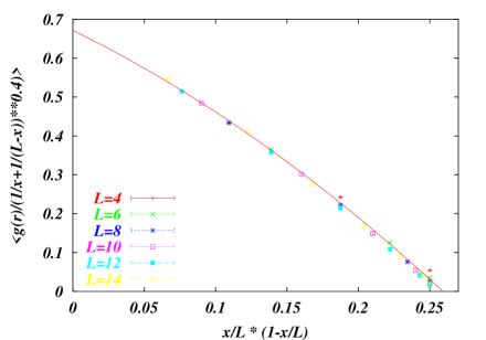
FIG. 3.: The overlap-overlap correlation function minus $q^{2}$ divided times the factor $\left(\frac{1}{x}+\frac{1}{L-x}\right)^{0.4}$ (i.e. the function $g$ defined in (1)) as a function of $w=\frac{x}{L}-\left(\frac{x}{L}\right)^{2}$. The line is for the best fit to a second order polynomial.

When we analyze the correlation function of the link overlap we also select events at a fixed value of $q^{2}$: as in the previous case we will consider a cut of the form $|q|<q_{max}=.1$. We only measure a simple correlation function of $1-q_{l}(i)$ (we only look at correlations in a given plane, and average the two contributions coming from separating in the direction $2$ links in the direction $1$ and in the direction $1$ links in the direction $2$ [4]), that we call $\Omega(x,L)$, which we plot in fig. 4 for various $L$ ($x\geq 1$). The different sets of points are plotted versus $s(x,L)\equiv(1/x+1/(L-x))^{\lambda}$. If we chose the value $\lambda=2.1$ the data at given $L$ can be very well fitted by a linear functions, i.e. the lines in fig. 4:

$$\Omega(x,L)=a(L)+b(L)\ s(x,L)\ .$$ (2)

We plot in fig. 5 $a(L)$ and $b(L)$ from (2) and the best linear fits. If for $L\to\infty$ $1-q_{l}(0)$ would go to zero, this correlation function should become identically zero and consequently the two functions, $a(L)$ and $b(L)$, should extrapolate to zero when $L\to\infty$. However the slope $b(L)$ does not show any tendency to go to zero: the fact that it increases (slightly) with $L$ is a substantial indication that it does not converge to zero in the infinite volume limit. The intercept is fitted very well by a $1/L$ behavior without corrections and it extrapolates to a non zero value. Moreover the correlation function at large distances should be the square of the expectation values and consequently we have the relation $a(L)|_{L=\infty}=(1-q_{l}(0))^{2}$. This relation gives a value of $1-q_{l}(0)=0.26\pm 0.02$, that compares very nicely to the values we have discussed earlier.

Let us start summarizing our results. We have applied a bulk perturbation, and shown that the results substantiate in a perfect way the ones obtained by changing the boundary conditions [4]. The quantity $1-q_{l}(0)$ has a non-zero value that compares very well to the one determined in [4]. We have also determined that $\overline{q_{l}}$ behaves very similarly, and we have estimated its value in the infinite volume limit (four different estimates, affected by different systematic errors are $.24\pm.01$, $.26\pm.02$, $.30\pm.01$, $.33\pm.02$, the errors being purely statistical). We have shown that very plausibly in the limit $L\to\infty$ $q_{l}$ is a well behaved function of $q^{2}$, in strict analogy to what happens in the mean field RSB theory. We have analyzed site overlap and link overlap spatial correlation functions, and we have shown they perfectly obey scaling laws implied by a RSB scenario. Again, this results is quantitative, in which it leads to an estimate of $q_{l}(0)$ coherent with the ones given before.

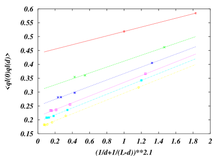
FIG. 4.: Points are for the link overlap auto correlation functions versus $w^{2.1}$. Lattice sizes are from $L=4$ (upper points and line) to $L=14$ (lower points and line). Lines are for linear best fits.

The RSB scenario is perfectly compatible with the whole set of data. These results are consistent with the recent detection of large scale excitations in spin glass ground states [10, 2]. The behavior we find connects smoothly with the results obtained by simulations at finite temperature [3] (e.g. the overlap-overlap correlation decays as the distance to a power $\phi=.4$, which is not far from the value obtained from simulation at finite temperature). We think that we have conclusively shown that the ground state structure of $3D$ Ising spin glasses with Gaussian quenched random couplings is not trivial.

EM thanks for the very nice hospitality the SPhT of Saclay CEA and the LPTMS of Université Paris Sud, Orsay, where part of this work has been done. We are grateful to O. Martin, M. Palassini and P. Young for useful correspondences and conversations.

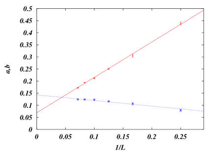
FIG. 5.: $a(L)$ (upper points) and $b(L)$ (lower points) from equation (2) and the two best linear fits.

REFERENCES

- [1] K. F. Pál, Physica A 223, 283 (1996); H. Rieger, in Lecture Notes in Physics 501 (Springer-Verlag, Heidelberg 1998); J. Houdayer and O. Martin, Phys. Rev. Lett. 83, 1030 (1999); M. Palassini and A. P. Young, Phys. Rev. Lett. 83, 5126 (1999).
- [2] M. Palassini and A. P. Young, cond-mat/0002134.
- [3] E. Marinari, G. Parisi, F. Ricci-Tersenghi, J.J. Ruiz-Lorenzo and F. Zuliani, J. Stat. Phys. 98, 973 (2000).
- [4] E. Marinari and G. Parisi, cond-mat/0002457, to be published on Phys. Rev. Lett.; cond-mat/0005047.
- [5] M. Mézard, G. Parisi and M. A. Virasoro, Spin Glass Theory and Beyond (World Scientific, Singapore 1987).
- [6] W. L. McMillan, J. Phys. C 17, 3179 (1984); A. J. Bray and M. A. Moore, in Heidelberg Colloquium on Glassy Dynamics and Optimization, L. Van Hemmen and I. Morgenstern eds. (Springer-Verlag, Heidelberg 1986); D. S. Fisher and D. A. Huse, Phys. Rev. B 38, 386 (1988).
- [7] M. A. Moore, H. Bokil and B. Drossel, Phys. Rev. Lett. 81, 4252 (1998); E. Marinari, G. Parisi, J.J. Ruiz-Lorenzo and F. Zuliani, Phys. Rev. Lett. 82, 5176 (1999); H. Bokil, A. J. Bray, B. Drossel M. A. Moore, Phys. Rev. Lett. 82, 5177 (1999).
- [8] F. Ricci-Tersenghi and F. Ritort, J. Phys. A 33, 3727 (2000).
- [9] H. G. Katzgraber, M. Palassini and A. P. Young, cond-mat/0007113.
- [10] J. Houdayer and O. Martin, cond-mat/9909203; F. Krzakala and O. C. Martin, cond-mat/0002055.
- [11] E. Marinari and G. Parisi, in preparation.
- [12] S. Franz and G. Parisi, cond-mat/0006188.
- [13] See for example C. de Dominicis, I. Kondor and T. Temesvari, in Spin Glasses and Random Fields, edited by A. P. Young (World Scientific 1998).