The Free Energy Surface of Supercooled Water

Abstract

We present a detailed analysis of the free energy surface of a well characterized rigid model for water in supercooled states. We propose a functional form for the liquid free energy, supported by recent theoretical predictions [Y. Rosenfeld and P. Tarazona, Mol. Phys. 95, 141 (1998)], and use it to locate the position of a liquid-liquid critical point at $T_{C^{\prime}}=130\pm 5$ K, $P_{C^{\prime}}=290\pm 30$MPa, and $\rho_{C^{\prime}}=1.10\pm 0.03$ g/cm³. The observation of the critical point strengthens the possibility that SPC/E water may undergo a liquid-liquid phase transition. Finally, we discuss the possibility that the approach to the liquid-liquid critical point could be pre-empted by the glass transition.

I introduction

The thermodynamic description of supercooled water has been a major research topic in recent years. Striking anomalies—such as the existence of a minimum in the isothermal compressibility $K_{T}$ along isobars, the increase of the isobaric specific heat $C_{P}$ on cooling, and the temperature of maximum density $T_{MD}$ along isobars—characterize the behavior of liquid water [1, 2, 3]. In particular, the study of supercooled states of water sheds light on the understanding of the anomalous behavior of liquid water. The increase of $K_{T}$ and $C_{p}$ on supercooling reinforces the possibility that the thermodynamic properties of supercooled water could be different from those of simple liquids. Speedy and Angell proposed a scenario in which the increase of $K_{T}$ and $C_{p}$ is related to a re-entrant spinodal line in the phase diagram of water by postulating the existence of an ultimate limit of stability for the liquid phase on cooling [4].

More recently, increased computing power has made possible the numerical study of the thermodynamic properties of models for water. In particular, supercooled states, where relaxation times increase by several orders of magnitude over typical liquid values, have become computationally accessible. It has been shown that explicit atom models (such as ST2 [5], TIP4P/TIP5P [6], and SPC/E [7]), as well as lattice [8] and continuum [9] models, are able to reproduce the anomalous thermodynamic properties of water. In all the atomistic models that have been studied, it has been found that the spinodal line is not re-entrant. Additionally, for the ST2 model, the existence of a novel liquid-liquid critical point has been directly observed in molecular dynamics simulations [10]. Hence, it has been proposed that the anomalous thermodynamic properties of liquid water could be related to a liquid-liquid phase transition. According to this hypothesis, two distinct forms of liquid water, separated by a first-order transition, may exist below a critical temperature $T_{c}$; such a critical point would account for the unusual increases in the thermodynamic response functions on cooling. Unfortunately, in water, the estimated $T_{c}$ is below the homogeneous nucleation temperature, i.e., inside the so-called “no-man’s land”. This notwithstanding, recent experiments [11] have probed the possible thermodynamic scenarios which characterize liquid water [3, 4, 10, 12].

From a simulation point of view, the ST2 model is the only one that allows a direct study of the liquid-liquid critical point; an increase of many orders of magnitude in computing power is needed for a direct detection of a critical point in other point charge models. Also, in supercooled states at the same $T$ and $P$, ST2 molecules are more mobile compared to real water. This feature has been exploited for equilibrating configurations at relatively low $T$ [10, 13]. The ST2 potential is over-structured compared to water, and the equation of state is shifted to higher values of pressure $P$, and temperature $T$ [10].

Among the molecular potentials which have been studied in detail, a significant role has been played by the extended simple point charge (SPC/E) model, both because of its simplicity and its success in capturing the properties of water in the bulk state [14, 15, 16, 17], as well as in biological systems [18]. The SPC/E model has three point charges, located at the atomic centers of the water molecule. SPC/E is under structured, with its equation of states shifted to lower values of P and T compared to water [14]. Also, in the supercooled regime, at the same $T$ and $P$, SPC/E molecules are less mobile than real water molecules [15, 16, 17]. Since it has been shown that the ST2 and SPC/E models bracket the thermodynamic behavior of water in the $T-P$ plane [14], it would be encouraging to clearly detect the presence of a liquid-liquid critical point also in the SPC/E potential. Unfortunately, the reduced diffusivity of SPC/E compared to ST2 makes it impossible to study directly the low $T$ and high $P$ region, where the SPC/E second critical point should be located.

Here we propose a functional form for the free energy surface of the SPC/E model in the low temperature region. Our work is supported by recent theoretical predictions for the $T$ dependence of the potential energy in supercooled states [19], which have been tested for several model liquids [20, 21, 23, 24]. The calculated functional form provides a good description of the thermodynamic quantities in the region where simulations are feasible, and predicts the presence of a liquid-liquid critical point $C^{\prime}$ at $T_{C^{\prime}}=130\pm 5$ K, $P_{C^{\prime}}=290\pm 30$MPa, and $\rho_{C^{\prime}}=1.10\pm 0.03$ g/cm³, in reasonable agreement with prior estimates [14] based on the characteristic shift in thermodynamics properties between the SPC/E and the ST2 model.

II The SPC/E Helmholtz Free Energy

The numerical data used to calculate the Helmholtz free energy $F=E-TS$ are obtained from the long molecular dynamics simulations of Ref. [16] for 42 different state-points, comprising 7 different densities and 6 different temperatures. The simulation results for the total energy $E$ and pressure $P$ are used here to reconstruct $F$ in the region $T>210$K, as we describe below. As noted in Ref. [14], the energy $E$ as a function of $V$ develops an increasingly pronounced convexity on lowering $T$. This signals the possibility of a phase transition, as $F=E-TS$ will be then also convex at low $T$.

Simulations of the SPC/E model below $T\approx 200$K are not feasible at the present time, as the time needed to observe equilibrium metastable properties exceeds currently available resources. Here, the simulation data for SPC/E water are limited to the region $T>200$K. To investigate the phase behavior at lower $T$, we exploit the recently-proposed relationship for the low-$T$ dependence of the potential energy $U$ along isochoric paths [19]. Specifically, the low-$T$ behavior of the potential energy is predicted to follow the functional form [19]

$$U_{\mbox{fit}}(T,V)=U_{0}(V)+\alpha(V)T^{3/5}.$$ (1)

Here $U_{0}$ represents the $T=0$ K value of $U_{\mbox{fit}}$, which for a classical system may also be identified with $F(0,V)$. The functional form of Eq. (1) has been shown to describe the temperature dependence of the potential energy in several different models, ranging from Lennard-Jones to Yukawa potentials [20, 21, 22, 23, 24]. Although no specific prediction has been presented until now for molecular systems, we find that in the temperature range between $T=200$ and $T=300$ K the SPC/E potential energy is very well described by the $T^{3/5}$ law, as shown in Fig. 1. The volume dependence of $U_{0}(V)$ and $\alpha(V)$ are reported in Fig. 2 and in Table I. Since $F(T=0,V)$ coincides with $U_{0}(V)$, the clear negative concavity of $U_{0}(V)$ at large volumes indicates that if the $T^{3/5}$ law would hold down to $T=0$K, then the extrapolated liquid free energy would imply a two-phase coexistence at zero temperature. As will be discussed in more detail later, at $T=0$K the two phases are separated by a first order transition around $P=380$ MPa.

Since the $V$ dependence of $U_{0}$ and $\alpha$ is smooth, we derive a functional form $U_{\mbox{fit}}(V,T)$, by fitting the values of $U_{0}(V)$ and $\alpha(V)$ with sixth degree polynomials $U_{0}(V)=\sum_{n=0}^{6}b_{n}V^{n}$ and $\alpha(V)=\sum_{n=0}^{6}a_{n}V^{n}$. We thus obtain

$$U_{\mbox{fit}}(T,V)=\sum_{n=0}^{6}a_{n}V^{n}+T^{3/5}\sum_{n=0}^{6}b_{n}V^{n}$$ (2)

The $a_{n}$ and $b_{n}$ values are reported in Table II. We find almost identical values of $U_{0}$ and $\alpha$ if we truncate Eq. (2) at order $V^{5}$. The resulting expression $E(V,T)=3k_{B}T+U_{\mbox{fit}}(V,T)$ for the total energy describes very well the simulation results, as shown in Fig. 3.

We obtain the entropy $S$ using the thermodynamic relation

$$S(T,V)=S(T_{0},V_{0})+\frac{1}{T}\int^{T,V}_{T_{0},V_{0}}(dE+PdV)$$ (3)

where the state point $(T_{0},V_{0})$ is some reference state point. We calculate the temperature-dependence of $S$ along isochores from Eq. (2), by performing thermodynamic integration along constant $V$ paths. $S(T,V)$ is given by

$$S(T,V) = S(T_{0},V)+\int_{T_{0}}^{T}\frac{dT}{T}\left(\frac{\partial E}{\partial T}\right)_{V}$$ (4)

$$= S(T_{0},V)+3k_{B}\ln\left(\frac{T}{T_{0}}\right)-\frac{3}{2}\alpha(V)\left(T^{-\frac{2}{5}}-T_{0}^{-\frac{2}{5}}\right).$$ (5)

The unknown $S(T_{0},V)$ function can be evaluated, at any chosen $T_{0}$, from the knowledge of the $V$-dependence of $P$ using Eq. 3. To calculate $S(T_{0},V)$ we fit the simulation data for $P(T=300$K$,V)$ again with a sixth-order polynomial

$$P_{\mbox{fit}}(T=300\mbox{K},V)=\sum_{n=0}^{6}c_{n}V^{n}.$$ (6)

The values of the resulting $c_{n}$ coefficients are reported in Table II. From elementary calculus,

$$S(T_{0},V) = S(T_{0},V_{0})-\frac{E(T_{0},V_{0})-E(T_{0},V)}{T_{0}}+$$ (8)

$$\sum_{n=0}^{6}\frac{c_{n}}{n+1}{V^{n+1}-V_{0}^{n+1}\over T_{0}}.$$

The only unknown quantity left is $F(T_{0},V_{0})$, which can be calculated, if needed, starting from a known reference point (as for example an ideal gas state, as done in ref. [21]) and performing thermodynamic integration up to $V_{0},T_{0}$. The resulting expression for $F(T,V)=E(T,V)-TS(T,V)$ can then be used to calculate thermodynamic properties of SPC/E water.

III Results

First, we compare in Figs. 3 and 4 the values of $E_{\mbox{fit}}=(1-T\partial/\partial T)F_{\mbox{fit}}$ and $P_{\mbox{fit}}=-\partial F_{\mbox{fit}}/\partial V$ with the simulation results for $T<300$K. Note that the derivatives eliminate the unknown constant $F(V_{0},T_{0})$. We also calculate the line of density maxima, $T_{MD}$, defined as the locus where $(\partial V/\partial T)_{P}=0$. The predicted line is compared with the results of the simulations in Fig. 6.

We next use the expression for $F$ to calculate the thermodynamic properties for $T<200$K where simulations are not feasible. The free energy expression proposed depends primarily on the assumption of the $T^{3/5}$ dependence of the potential energy in supercooled states. The theoretical prediction and the quality of the $T^{3/5}$ description reported in Fig. 1 suggests that we may meaningfully extrapolate the calculation to a temperature lower than the one for which equilibration is feasible at the present time, and search for the possibility of a liquid-liquid critical point.

We calculate $P_{\mbox{fit}}$ and find that, at temperatures lower than $130\pm 5$K, a van der Waals loop (Fig. 5) develops, signaling a first-order transition between two liquid phases. The common tangent construction [25] for the Helmholtz free energy $F_{\mbox{fit}}$ allows us to calculate the coexistence line; further, we calculate the spinodal lines $(\partial P_{\mbox{fit}}/\partial V)_{T}=0$. The coexistence line meets the spinodal at a critical point $C^{\prime}$, which we find at $T_{C^{\prime}}=130\pm 5$K, $P_{C^{\prime}}=290\pm 30$ MPa, and $\rho_{C^{\prime}}=1.10\pm 0.03$ g/cm³.

The resulting SPC/E phase diagram is shown in Fig. 6 in both the $(P-T)$ and $(\rho-T)$ planes. Fig. 6 also shows the recently-calculated Kauzmann temperature $T_{K}$ locus [21], defined as the temperature at which the configurational entropy vanishes [26]. The evaluation of the Kauzmann locus is also based on the assumption that the system potential energy has a $T^{3/5}$-dependence, and hence is fully consistent with the present free energy calculations. We note that the predicted critical temperature is $\approx 10$K below the Kauzmann temperature where SPC/E water is predicted to have a vanishing diffusivity [21].

As a final consideration, we discuss the interplay between the location of the critical point and the Kauzmann line. Since at the Kauzmann line the configurational entropy vanishes, all equilibrium thermodynamic calculations lose meaning below this line. In this sense, the critical point in the SPC/E phase diagram should not be considered. In the potential energy landscape paradigm [26, 27, 28, 29], the system would be trapped in a single basin reached at $T_{K}$. None-the-less, the free energy below $T_{K}$ can still be calculated by considering its separate parts. The contribution to the free energy due to the multiplicity of basins sampled would be fixed at its value at $T_{K}$, i.e. zero. Thus, below $T_{K}$ the intra-basin free energy coincides with $F$. At low T, frequently, a model based on a harmonic solid is appropriate for such a calculation [20, 21, 22]. The ‘free energy calculated will still display a critical point (but slightly shifted compared to the present estimate) since the basic mechanism which gives rise to the low-$T$ instability is the shape of $E(V,T)$, which is already convex well above $T_{K}$.

IV Conclusions

In this article, we have presented a technique of evaluating thermodynamic quantities in the supercooled region, in a $T$-range where equilibrium simulations are not feasible due to extremely long equilibration times. The relevant result of this analysis, applied to the SPC/E potential, is a clear indication that the free energy surface develops a region of negative curvature on cooling. A liquid-liquid critical point develops, in analogy with the behavior of the ST2 model, for which the location of the critical point is within the region where equilibrated configurations can be calculated.

The predictions reported in this manuscript are based on a functional form for the liquid free energy, supported by recent theoretical predictions [19]. Of course, changes in the temperature dependence related to novel phenomena which may take place outside the range where data are available may break the validity of the extrapolation. In the case of real water, for example, it has been argued that a change in the $T$-dependence of the thermodynamic properties takes place in the “no-man’s land” [30]. In the case of SPC/E water, if such change takes place, it must occur at $T\lesssim 200K$, i.e. in the region where simulations are not feasible. This would effect our estimate of the location of the critical point. However, the existence of a region of negative curvature already in the $T$-region where simulations are feasible supports the possibility that the liquid-liquid critical transition would take place at lower temperatures, independently from the assumed $T^{3/5}$ law.

Our results have a particular relevance, since, as previously noticed, ST2 and SPC/E typically bracket the thermodynamic behavior of the real liquid. The evidence presented here that the SPC/E potential displays a critical point at low $T$ and high $P$ strengthens the possibility that, below the homogeneous nucleation temperature, water may undergo a liquid-liquid (or glass-glass) phase transition; the two distinct liquid phases that would appear below $C^{\prime}$ could correspond to the two observed amorphous forms of solid water, low density amorphous and high density amorphous ice. Indeed, such a transition could be observed in the glassy state even if $T_{C^{\prime}}<T_{K}$, as we find for the SPC/E model.

The thermodynamic analysis presented here also allows us to grasp the origin of the presence of the critical point. Indeed, the presence of the critical point arises from the negative concavity of $E(T,V)$, which for $T>T_{C}$ is compensated by the $-TS(T,V)$ contribution. Note that, as previously observed [10], the negative concavity of $E(T,V)$ already appears in the $T$-region where equilibrium simulations are feasible, suggesting an inevitable phase transition as the product $TS$ becomes progressively smaller with decreasing $T$. Such negative concavity of $E(V,T)$ is also found in supercooled water [31].

V Acknowledgments

F.W.S. is supported by the National Research Council. F.S. acknowledges support from INFM-PRA-HOP, Iniziativa Calcolo Parallelo, and MURST-PRIN-98. This work was also supported by the NSF.

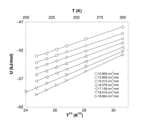
FIG. 1.: Fit of the potential energy along isochores with the functional form $U_{0}+\alpha T^{3/5}$. Symbols denote different molar volumes. For sake of clarity, the different isochores are shifted by -1 kJ/mol each in order to avoid overlaps.

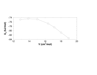
FIG. 2.: The volume dependence of $U_{0}(V)$ from eq. (2). Note that this coincides with $F(T=0$  $\mbox{K},V)$. The negative curvature implies the presence of an unstable region in the phase diagram at low $T$.

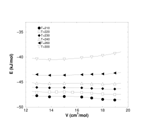
FIG. 3.: Comparison between the energy E calculated from simulations [14] and from the free energy approach described here.

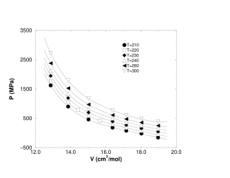
FIG. 4.: Comparison between pressures as calculated from Fig. 3.

FIG. 5.: Pressure at $T=100$K as calculated. The equilibrium pressure is obtained by the Maxwell construction.

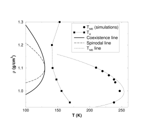
FIG. 6.: P-T (upper panel) and $\rho$-T (lower panel) phase diagrams. The coexistence line, the spinodals and the $T_{MD}$ line from our free energy. Squares are $T_{MD}$ points obtained from simulations; the triangles are the Kauzmann boundary [26] for SPC/E water [21] below which diffusivity is predicted to vanish [27].

TABLE I.: Fitting parameters for the potential energy to Eq. (1). The fits are made for $210$ K $\leq T\leq 300$ K.

$V$ (cm3/mol)	$U_{0}$ (kJ/mol)	$\alpha$ (kJ/(mol$\cdot$K3/5))
18.96421	-83.41894	1.1970260
18.01600	-80.86653	1.1000960
17.15810	-78.47431	1.0130790
16.37818	-76.65199	0.9468765
15.01333	-74.77946	0.8767148
13.85846	-74.50920	0.8653371
12.86857	-74.91184	0.8835562

TABLE II.: Polynomial fitting coefficients for $U_{0}(V)$, $\alpha(V)$ (see Eq. (2)) and for $P(T=300K,V)$ (Eq. 6). Note that the dimensions of the coefficients depend on the term $n$ of the expansion.

$n$	$a_{n}$ (kJ$\cdot$moln-1/cm3n)	$b_{n}$ (kJ$\cdot$moln-1/(K${}^{3/5}\cdot$cm3n)	$c_{n}$ (MPa$\cdot$moln/cm3n)
0	$76.617$	$-1.8261$	$6.8671\times 10^{4}$
1	$-30.435$	$0.61927$	$2.4466\times 10^{3}$
2	$1.279.8$	$-2.9301\times 10^{-2}$	$2.8096\times 10^{3}$
3	$5.0719\times 10^{-2}$	$-9.6397\times 10^{-4}$	$3.0755\times 10^{2}$
4	$4.4964\times 10^{-5}$	$-2.63884\times 10^{-5}$	$1.2970\times 10^{1}$
5	$-3.7530\times 10^{-4}$	$1.07393\times 10^{-5}$	$0.1871$
6	$1.1301\times 10^{-5}$	$-3.1252\times 10^{-7}$	$3.4974\times 10^{-4}$

REFERENCES

- [1] C. A. Angell, in Water: A Comprehensive Treatise, edited by F. Franks (Plenum, New York, 1981).
- [2] P. G. Debenedetti, Metastable Liquids (Princeton Univ. Press, Princeton, 1996).
- [3] O. Mishima and H. E. Stanley, Nature 396, 329 (1998).
- [4] R. J. Speedy and C. A. Angell, J. Chem. Phys. 65, 851 (1976); R. J. Speedy, J. Chem. Phys. 86, 892 (1982).
- [5] F.H. Stillinger and A. Rahman, J. Chem. Phys. 60, 1545 (1974).
- [6] W.L. Jorgensen, J. Chandrasekhar, J. Madura, R.W. Impey, and M. Klein, J. Chem. Phys 79 926 (1983); M.W. Mahoney and W.L. Jorgensen, J. Chem. Phys., 112 8910 (2000).
- [7] H. J. C. Berendsen, J. R. Grigera, and T. P. Stroatsma, J. Phys. Chem. 91, 6269 (1987).
- [8] H. E. Stanley and J. Teixeira, J. Chem. Phys. 73, 3404 (1980); S. Sastry, F. Sciortino, and H.E. Stanley, J. Chem. Phys. 98, 9863 (1993); S. Sastry, F. Sciortino, P. G. Debenedetti, and H. E. Stanley, Phys. Rev. E 53, 6144 (1996); L. P. N. Rebelo, P. G. Debenedetti, and S. Sastry, J. Chem. Phys. 109, 626 (1998); C. J. Roberts, A. Z. Panagiotopoulos, and P. G. Debenedetti, Phys. Rev. Lett. 97, 4386 (1996); C. J. Roberts and P. G. Debenedetti, J. Chem. Phys. 105, 658 (1996).
- [9] P.H. Poole, F. Sciortino, T. Grande, H.E. Stanley, and C.A. Angell, Phys. Rev. Lett. 73, 1632 (1994); T.M. Truskett, P.G. Debenedetti S. Sastry, and S. Torquato, J. Chem. Phys. 111, 2647 (1999).
- [10] P. H. Poole, F. Sciortino, U. Essmann, and H. E. Stanley, Nature 360, 324 (1992); Phys. Rev. E 48, 3799 (1993); S. Harrington, R. Zhang, P.H. Poole, F. Sciortino, and H.E. Stanley, Phys. Rev. Lett. 78, 2409 (1997); F. Sciortino, P.H. Poole, U. Essmann, and H.E. Stanley, Phys. Rev. E 55, 727 (1997);
- [11] O. Mishima and H. E. Stanley, Nature 392, 192 (1998); O. Mishima, Phys. Rev. Lett. 85, 334 (2000).
- [12] S. Sastry, F. Sciortino, P. G. Debenedetti, and H. E. Stanley, Phys. Rev. E 53, 6144 (1996); L. P. N. Rebelo, P. G. Debenedetti, and S. Sastry, J. Chem. Phys. 109, 626 (1998); E. La Nave, S. Sastry, F. Sciortino and P. Tartaglia Phys. Rev. E 59 6348-6356 (1999).
- [13] D. Paschek and A. Geiger, J. Phys. Chem. B 103, 4139 (1999).
- [14] S. Harrington et al., J. Chem. Phys. 107, 7443 (1997).
- [15] F. Sciortino, P. Gallo, P. Tartaglia, S.-H. Chen, Phys. Rev. E 54, 6331 (1996); P. Gallo, F. Sciortino, P. Tartaglia, and S.-H. Chen, Phys. Rev. Lett. 76, 2730 (1996).
- [16] F. W. Starr et al., Phys. Rev. Lett. 82, 3629 (1999); Phys. Rev. E 60, 6757 (1999).
- [17] F. Sciortino, Chem. Phys. 258 295-302 (2000).
- [18] M. Tarek and D.J. Tobias (preprint).
- [19] Y. Rosenfeld and P. Tarazona, Mol. Phys. 95, 141 (1998)
- [20] F. Sciortino, W. Kob, and P. Tartaglia, Phys. Rev. Lett. 83, 3214 (1999); B. Coluzzi, P. Verrochio, and G. Parisi, Phys. Rev. Lett 84, 306 (2000).
- [21] A. Scala, F. W. Starr, E. La Nave, F. Sciortino, and H. E. Stanley, Nature 406, 166 (2000).
- [22] F.W. Starr, S. Sastry, E. La Nave, A. Scala, F. Sciortino, and H.E. Stanley, cond-mat/0007487.
- [23] S. Sastry, Phys. Rev. Lett. 85 590 (2000).
- [24] I. Saika-Voivod, F. Sciortino, P. H. Poole, cond-mat/0007380.
- [25] L.D. Landau and E.M. Lifshits, Statistical Physics (Addison-Wesley, Reading, 1969).
- [26] W. Kauzmann, Chem. Rev. 43, 219 (1948).
- [27] G. Adam and J.H. Gibbs, J. Chem. Phys. 43, 139 (1965).
- [28] M. Goldstein, J. Chem. Phys. 51, 3728 (1969).
- [29] F.H. Stillinger and T.A. Weber, Phys. Rev. A, 25 978 (1982); F.H. Stillinger and T.A. Weber, Science 225 983 (1984). F. H. Stillinger, Science, 267, 1935, (1995).
- [30] C.A. Angell, J. Phys. Chem. 97, 6339 (1993); K. Ito, C.T. Moynihan, and C.A. Angell, Nature 398, 492 (1999); F.W. Starr, C.A. Angell, R.J. Speedy, and H.E. Stanley, cond-mat/9903451; R. Bergman and J. Swenson, Nature 403, 283 (2000); R.S. Smith and B.D. Kay, Nature 398, 288 (1999).
- [31] L.Haar, J.S.Gallagher and G.Khel, NBS/NRC Steam Tables, (Hemisphere, Washington DC, 1985).