Exact Solution of the strong coupling t-V model
with twisted boundary conditions

Abstract

We present the solution of the one-dimensional t-V model with twisted boundary conditions in the strong coupling limit, $t\ll V$ and show that this model can be mapped onto the strong coupling Hubbard chain threaded by a fictitious flux proportional to the total momentum of the charge carriers. The high energy eigenstates are characterized by a factorization of degrees of freedom associated with configurations of soliton and antisoliton domains and degrees of freedom associated with the movement of “holes” through these domains. The coexistence of solitons and antisolitons leads to a strange flux dependence of the eigenvalues. We illustrate the use of this solution, deriving the full frequency dependence of the optical conductivity at half-filling and zero temperature.

]

I Introduction

The extended Hubbard model and its spinless version, the t-V model, have been extensively studied due to their relevance in the comprehension of the behavior of strongly correlated compounds such as cuprates[1, 2, 3] and organic conductors. [4, 5] Much of the present understanding of these models has been a consequence of the exact solution in one dimension by the Bethe ansatz (BA) technique. [6, 7] The evaluation of the correlations remains however a hard task within the Bethe ansatz framework. For the Hubbard model, further progress was possible in the strong coupling limit due to the simpler form of the solution. [8, 9, 10, 11, 12] The eigenfunctions in this limit factorize as a product of a wavefunction of non-interacting spinless fermions and a wavefunction of a squeezed spin chain.[8, 13] This spin-charge factorization simplifies the calculation of correlations and in particular, it has been used to determine the momentum distribution function,[8] the spectral function,[9, 10] the sum rules of the upper and lower Hubbard bands [11] and the Green’s function [12] of this model. An alternative solution to that of the Bethe ansatz was also possible in this limit.[13, 14, 15]

The t-V model is apparently simpler than the Hubbard model due to the absence of spin degrees of freedom. This model can be mapped onto the anisotropic Heisenberg model (more precisely, the XXZ or Heisenberg-Ising model) by the Jordan-Wigner transformation,[16] whose Bethe ansatz solution has long been known.[17] In the strong coupling limit, the t-V model, despite its apparent simplicity, remains somewhat foggier than the Hubbard model. For instance, the Bethe ansatz solution[18, 19, 20] presents us eigenvalues expressions with phase terms whose physical meaning is not clear. Another curious fact is that the Luttinger liquid exponent[21] that characterizes the low energy excitations of the strong coupling t-V model is density dependent [22] in contrast to the strong coupling Hubbard model where it is a constant. [2] Since this exponent is closely related to Fermi surface phase shifts (a holon Fermi surface in the case of the Hubbard model),[2] it is worthwhile to investigate how these phase shifts will be modified. In this paper, we present a non-Bethe-ansatz solution for the strong coupling one-dimensional t-V model which is closely related to the solution of the strong coupling Hubbard model [14] and which clarifies the previous issues. The simple factorized form of this solution (and the low degeneracy of the eigenvalues) will, we believe, allow an easy calculation of correlations.

The t-V Hamiltonian for a ring with $L$ sites is

$$H=-t\sum_{i}(c_{i}^{\dagger}c_{i+1}+c_{i+1}^{\dagger}c_{i})+V\sum_{i}n_{i}n_{i+1},$$ (1)

where $c_{i}^{\dagger}$ is the fermion creation operator on site $i$, $n_{i}=c_{i}^{\dagger}c_{i}$ and $V$ is the nearest-neighbor Coulomb interaction. The one-dimensional strong coupling t-V model (as the Hubbard model) is a classic example of a system which exhibits a metal-insulator transition upon doping. If $t=0$, the fermions are localized and all states with the same number of pairs of nearest-neighbor occupied sites, $\sum_{i}n_{i}n_{i+1}$, are degenerate. This degeneracy is lifted if $t/V$ is finite and up to first order in $t$, the eigenvalues are obtained diagonalizing the Hamiltonian within each of the degenerate subspaces. In the strong coupling limit $t\ll V$, we obtain therefore the projected Hamiltonian

$$H = -t\sum_{i}[(1-n_{i+2})c_{i+1}^{\dagger}c_{i}(1-n_{i-1})+hc]$$ (4)

$$-t\sum_{i}[n_{i+2}c_{i+1}^{\dagger}c_{i}n_{i-1}+hc]$$

$$+V\sum_{i}n_{i}n_{i+1}.$$

This limit corresponds to the $J_{x}=J_{y}\ll J_{z}$ limit of the anisotropic Heisenberg model. The set of eigenstates and eigenvalues of this model can be obtained without having to resort to the Bethe ansatz, as we will show below.

The behavior of the t-V model in the strong coupling limit has provided support for a recent conjecture by Zotos and Prelovsek. [23, 24, 25] According to these authors, the t-V model and the Hubbard model at half-filling are perfect insulators, this meaning that the Drude weight ($D_{c}$) in the thermodynamic limit remains zero even at finite temperature. In particular, in the strong coupling limit, they argue that $D_{c}=0$ even for finite systems. Such behavior was confirmed by Peres et al, [18] applying the Bethe ansatz method to solve the t-V model in the strong coupling limit. Here, we present a different solution which allows an easy confirmation of the previous results and makes clearer the physical picture in this limit.

The remaining part of this paper is organized in the following way. In section II, the low energy eigenstates of the model are found. First, we study the one-particle problem and present a new path for its solution. Then, we show that this solution can be extended to the case with $N$ particles. We also find the flux dependence of the eigenvalues. In section III, the general solution is presented both for periodic and twisted boundary conditions (finite flux). We also comment on the higher order corrections. In section IV, we compare our results with those obtained with the Bethe ansatz technique. The transport properties of the model are studied in section V. Finally, we conclude in section VI.

II low energy subspace

Let us consider two consecutive sites and therefore, nearest neighbors of each other. There are four different configurations for this pair of sites, which we will call links and they are

$$(\bullet\,\bullet);(-\,\bullet);(\bullet\,-);(-\,-)$$ (5)

where a dot stands for an occupied site and a dash for an empty one. The total number of these links in the chain is equal to the number of sites $L$,

$$N_{\bullet\,\bullet}+N_{-\,\bullet}+N_{\bullet\,-}+N_{-\,-}=L$$ (6)

and $N_{-\,\bullet}=N_{\bullet\,-}$. Further conditions result from counting the number of holes or particles,

$$N_{-\,\bullet}+N_{-\,-} = N_{h},$$ (7)

$$N_{\bullet\,\bullet}+N_{-\,\bullet} = N_{e}.$$ (8)

In the limit $V/t\rightarrow\infty$, the number of links $(\bullet\,\bullet)$ is a conserved quantity and consequently also are $N_{-\,\bullet}$ and $N_{-\,-}$. So, in the strong coupling limit, the model merely exchanges the positions of these links. Note that $\sum_{i}n_{i}n_{i+1}=N_{\bullet\,\bullet}$.

A One particle

Let us start with the simple case of a single particle in our periodic chain. In this case, the interaction term is zero and we have a one-particle tight-binding model, whose solution is trivial. We are going to solve this model in a different fashion, considering as our mobile particle the link $(-\,\bullet)$. This link moves exchanging its position with a link $(-\,-)$. Note that we have one link $(-\,\bullet)$ and $L-2$ links $(-\,-)$, and therefore, the total number of these links is $\tilde{L}=L-1$.

First, let us define our states in terms of the position of this link,

$$|\tilde{i}\rangle=c_{i+1}^{\dagger}|0\rangle$$ (9)

with $1\leq\tilde{i}\leq L-1$. Note that there is a state $c_{1}^{\dagger}|0\rangle$ which is not included in the previous set of states, but this state can be written as

$$\hat{T}^{-1}|\tilde{1}\rangle=\hat{T}^{-1}c_{2}^{\dagger}|0\rangle$$ (10)

where $\hat{T}$ is the one-site translation operator. The single particle Hamiltonian rewritten using this new notation becomes

$$H/(-t)=\sum_{\tilde{i}\neq\tilde{L}}|\tilde{i}+1\rangle\langle\tilde{i}|+\hat{T}^{-1}|\tilde{1}\rangle\langle\tilde{L}|+h.c.$$ (11)

with $\tilde{L}=L-1$. We now introduce an over-complete set of states, constructing from a state $|\tilde{i}\rangle$, a state invariant by translation with momentum $k$,

$$|\tilde{i},k\rangle={1\over\sqrt{L}}\sum_{j=1}^{L}e^{ikj}\hat{T}^{j-1}|\tilde{i}\rangle.$$ (12)

These states diagonalize the Hamiltonian, but we are going to proceed as if they did not and as if they were an orthogonal set of states. The Hamiltonian becomes

$$H/(-t) = \sum_{k}\Big{(}\sum_{\tilde{i}\neq\tilde{L}}|\tilde{i}+1,k\rangle\langle\tilde{i},k|$$ (14)

$$+e^{ik}|\tilde{1},k\rangle\langle\tilde{L},k|+h.c.\Big{)}$$

The Hamiltonian in a given $k$ subspace has become that of a tight-binding model in a chain of $L-1$ sites with a fictitious flux $e^{ik}$. The eigenvalues are given by

$$E(\tilde{k},k)=-2t\cos\left(\tilde{k}-{k\over\tilde{L}}\right)$$ (15)

with $\tilde{k}=\tilde{n}\cdot 2\pi/\tilde{L}$, $\tilde{n}=0,\dots\tilde{L}-1$ and $k=n\cdot 2\pi/L$, $n=0,\dots L-1$. But clearly, not all combinations of $\tilde{k}$ and $k$ correspond to real eigenstates of the Hamiltonian. The eigenstates will be of the form

$$|\tilde{k},k\rangle={1\over\sqrt{\tilde{L}}}\sum_{j=1}^{\tilde{L}}e^{i(\tilde{k}-{k\over\tilde{L}})j}|\tilde{j},k\rangle,$$ (16)

but obviously, this is a combination of states which are the same state except for a phase, that is,

$$|\tilde{j},k\rangle=e^{ik}|\tilde{j}+1,k\rangle$$ (17)

and the linear combination will be zero unless the following condition is satisfied

$$\tilde{k}-{k\over\tilde{L}}-k=0\quad(\text{mod}\,\,2\pi)$$ (18)

which implies $\tilde{k}=kL/\tilde{L}\,\,(\text{mod}\,\,2\pi)$. This condition is equivalent to stating that the final state must obviously have a momentum $k$. Note that the previous equation has precisely $L$ solutions and therefore, the usual set of tight-binding eigenvalues is recovered.

Let us make a few remarks concerning the above procedure. Let $\{|i\rangle\}$, $i=1,\dots L$, be an orthogonal set of states which constitutes a basis for the states of a given system and let $H_{ij}$ be the matrix elements of the system Hamiltonian between the states $|i\rangle$ and $|j\rangle$. The set of eigenstates $\{|\phi_{i}\rangle\}$, $i=1,\dots L$, of the Hamiltonian can be written in this basis as $|\phi\rangle=\sum_{j}a_{j}|j\rangle$. Assume now that two or more states of this basis were in fact the same state. This would lead to a reduced matrix $\tilde{H}_{ij}$ which would have the same elements, except for the transitions to and from the state which remained from the set of equivalent states. These transitions are multiplied by the total number of equivalent states. The eigenstates of $H$ remain eigenstates of $\tilde{H}$, but now they constitute an over-complete basis of the Hilbert space, that is, they are not all linearly independent. They may however remain an orthogonal set if the states in excess are identically zero as in the case studied above.

B several particles

Let us consider now the case of $N_{e}$ particles in a chain of $L$ sites, but distributed so that there are no links $(\bullet\,\bullet)$. These states are of the form

$$|a_{1},\dots,a_{N_{e}}\rangle=\prod_{i=1}^{N_{e}}(1-n_{a_{i}-1})c_{a_{i}}^{\dagger}|0\rangle$$ (19)

with $\{a_{i}\}$ an ordered set of non-consecutive numbers ($a_{1}>1$). The total number of $(-\,-)$ and $(-\,\bullet)$ links is $\tilde{L}=L-N_{e}$. This state can be mapped onto the following state of a chain with $L-N_{e}$ sites,

$$|\tilde{a}_{1},\dots,\tilde{a}_{N_{e}}\rangle=\prod_{i=1}^{N_{e}}\tilde{c}_{\tilde{a}_{i}}^{\dagger}|\tilde{0}\rangle$$ (20)

such that if the first site of this pseudo-chain is empty, the first link of the $L$ sites chain is $(-\,-)$, if it is occupied, the first link is $(-\,\bullet)$. The same reasoning applies to the other sites. Note that as in the previous case, there are a few states which are not included in the above set, namely states where a link $(-\,\bullet)$ is divided between sites $L$ and $1$. These states have a particle at site $1$ and one should note that starting from a state as above, these states appear when a link $(-\,\bullet)$ is at site $\tilde{L}$, or equivalently, a particle is at site $L$ and hops to site $1$. However, this hopping term can written as

$$\hat{T}^{-1}\tilde{c}_{\tilde{1}}^{\dagger}\tilde{c}_{\tilde{L}}|\tilde{a}_{1},\dots,\tilde{a}_{N_{e}-1},\tilde{L}\rangle$$ (21)

where $\hat{T}$ is the one-site translation operator in the chain of $L$ sites. Note that this translation operator also insures that the other pseudo-particles remain in the same sites in the reduced chain. Given a state $|\tilde{a}_{1},\dots,\tilde{a}_{N_{e}}\rangle$, we build as previously the state invariant by translation with momentum $P$,

$$|\tilde{a}_{1},\dots,\tilde{a}_{N_{e}},P\rangle={1\over\sqrt{L}}\sum_{j=1}^{L}e^{iPj}\hat{T}^{j-1}|\tilde{a}_{1},\dots,\tilde{a}_{N_{e}}\rangle.$$ (22)

The mapped Hamiltonian in the subspace of states with momentum $P$ becomes

$$H(P)=-t\left(\sum_{\tilde{i}\neq\tilde{L}}\tilde{c}_{\tilde{i}+1}^{\dagger}\tilde{c}_{\tilde{i}}+e^{iP}\tilde{c}_{\tilde{1}}^{\dagger}\tilde{c}_{\tilde{L}}\right)+hc.$$ (23)

So, we have mapped the Hamiltonian onto a tight-binding chain with $L-N$ sites threaded by a flux $P$ with $N_{e}$ particles. The eigenvalues are given by

$$E(\{\tilde{k}\},P)=-2t\sum_{i=1}^{N_{e}}\cos\left(\tilde{k}_{i}-{P\over\tilde{L}}\right)$$ (24)

with $\tilde{k}=\tilde{n}\cdot 2\pi/\tilde{L}$, and $P=n\cdot 2\pi/L$, with $\tilde{n}=0,\dots,\tilde{L}-1$ and $n=0,\dots,L-1$. Again, not all combinations of pseudo-momenta $\{\tilde{k}\}$ and $P$ are possible and applying the same procedure as before, we arrive to following condition

$$\sum_{i=1}^{N_{e}}(\tilde{k}_{i}-{P\over\tilde{L}})-P=0\quad(\text{mod}\,\,2\pi)$$ (25)

which implies

$$P{L\over\tilde{L}}=\sum_{i=1}^{N_{e}}\tilde{k}\quad(\text{mod}\,\,2\pi).$$ (26)

The factor $L/\tilde{L}$ converts the total momentum of our chain of $L$ sites in the total momentum of the pseudo-chain. Note that the set of pseudo-momenta $\{\tilde{k}\}$ is not enough to define the total momentum $P$ since there may be two values of $P$ such that $PL/\tilde{L}$ (mod $2\pi$) is the same. In fact, if $P=n\cdot 2\pi/L$ , with $n=0,\dots,L-1$, the states $|\{\tilde{k}\},P\rangle$ with $n$ in the interval $[0,L-1-\tilde{L}]$ have the same energy as the states $|\{\tilde{k}\},P+{2\pi\tilde{L}\over L}\rangle$. In the particular case of $\tilde{L}=L/2$, given a state with momentum $P$, one always has a state with momentum $P+\pi$ with the same set of wavenumbers. The $\tilde{L}=L/2$ case corresponds to the half filling and indeed one knows that the ground state is doubly degenerate, one state having zero momentum, the other $\pi$. This is also valid for excited states (with $N_{\bullet\,\bullet}\neq 0$), as we shall see in the next section.

An external magnetic flux $\phi$ can be introduced in the problem with the transformation $t\rightarrow te^{i\phi/L}$. The Hamiltonian remains invariant by translation and all the previous steps can be repeated, leading to the following modification in the eigenvalue expression

$$E(\{\tilde{k}\})\rightarrow E\left(\left\{\tilde{k}-{\phi\over L}\right\}\right).$$ (27)

The ground state energy is given by Eq. 24. If $N_{e}$ is odd, all single-particle states with pseudo-momentum $\tilde{k}$ between $\pm 2\pi/\tilde{L}\cdot(N_{e}-1)/2$ are occupied and $\sum\tilde{k}=0$. Therefore,

$$E_{gs}^{odd} = -2t\sum_{i=-{N_{e}-1\over 2}}^{{N_{e}-1\over 2}}\cos\left({2\pi\over\tilde{L}}i\right)$$ (28)

$$= -2t{\sin\left({\pi N_{e}\over\tilde{L}}\right)\over\sin\left({\pi\over\tilde{L}}\right)}.$$ (29)

If $N_{e}$ is even, all states with $\tilde{k}$ between $-2\pi/\tilde{L}\cdot(N_{e}-2)/2$ and $2\pi/\tilde{L}\cdot N_{e}/2$ or between $-2\pi/\tilde{L}\cdot N_{e}/2$ and $2\pi/\tilde{L}\cdot(N_{e}-2)/2$ are occupied and $\sum\tilde{k}=\pm\pi/\tilde{L}\cdot N_{e}/L$. So,

$$E_{gs}^{even} = -2t\sum_{i=-{N_{e}-2\over 2}}^{N_{e}/2}\cos\left({2\pi\over\tilde{L}}i-{\pi\over\tilde{L}}{N_{e}\over L}\right)$$ (30)

$$= -2t{\sin\left({\pi N_{e}\over\tilde{L}}\right)\over\sin\left({\pi\over\tilde{L}}\right)}\cos\left({\pi\over L}\right).$$ (31)

This slight energy difference between the two cases had already been pointed out by Kusmartsev. [20] In the presence of a small flux $\phi$, the $N_{e}$ odd expression should be multiplied by a factor $\cos(\phi/L)$, while for $N_{e}$ even, a $-\phi/L$ term should be summed to the argument of the cosine.

This phase shift between the wavenumbers of the ground states with $N$ and $N+1$ particles should be responsible for the orthogonality catastrophe in the thermodynamic limit which, for example, leads to a zero renormalization constant $Z$ characteristic of a Luttinger liquid [21] (see Ref. [2] for a detailed calculation in the case of the strong coupling Hubbard model). The renormalization constant $Z$ is given by the overlap between the ground state with $N+1$ particles and the ground state with $N$ particles plus a particle at Fermi momentum,

$$Z=|\langle\psi_{GS}(N+1;P=k_{f})|c^{\dagger}_{k_{F}\sigma}|\psi_{GS}(N;P=0)\rangle|^{2}$$ (32)

yielding zero in the thermodynamic limit. Our results above indicate that the phase shift depends on the density, $\delta=\pi{N_{e}\over L}=\pi\rho$. Recall that in the case of the strong coupling Hubbard model, the phase shift of the holons wavenumbers is independent of the band filling, $\delta={\pi\over 2}$. That phase shift results from a $(-k_{F})$ momentum contribution from the spin sector.[2] Here, the phase shift is due to the total momentum of the charge carriers. This dependence on the band filling is in agreement with the fact that the anomalous exponent of this model is indeed band filling dependent. [22] The Luttinger liquid velocities[21] that characterize the low lying excitations have been found by Gomez-Santos [22] for the strong coupling t-V model in the thermodynamic limit based on very simple arguments (basically, the reduction of the effective size of the chain). These velocities and its finite size corrections are easily obtained from the previous equations. In the large $L$ limit, the Gomez-Santos results are reproduced:

$$v_{N}={L\over\pi}{\partial^{2}E_{T}\over\partial N^{2}}={2t\over(1-\rho)^{3}}\sin\left({\rho\pi\over 1-\rho}\right)$$ (33)

$$v_{J}={L\over\pi}{\partial^{2}E_{T}\over\partial\phi^{2}}=2t\left(1-\rho\right)\sin\left({\rho\pi\over 1-\rho}\right)$$ (34)

$$v_{S}=\sqrt{v_{N}v_{J}}={2t\over(1-\rho)}\sin\left({\rho\pi\over 1-\rho}\right)$$ (35)

where $\rho={N_{e}\over L}$ and $v_{N}$, $v_{J}$, and $v_{S}$ are respectilvely the particle, current, and sound-wave velocities.

III general solution

Let us consider the general case where one may have both links $(\bullet\,\bullet)$ and $(-\,-)$. First, note that a phase separated state (one domain of holes and one domain of particles) has no mobile entities in the strong coupling limit since any hopping of a single particle would imply the breakup of a link $(\bullet\,\bullet)$. So, phase separated states will be eigenstates of the strong coupling Hamiltonian with eigenvalues given by $E=V\cdot N_{\bullet\,\bullet}$. Furthermore, the same applies to states with several domains if the only links $(-\,\bullet)$ present are the domain walls. Clearly, a hole (particle), in order to be able to move, must be within a particle (hole) domain. If for a chain with $L$ sites and $N_{e}$ particles, we fix $N_{\bullet\,\bullet}$ and $N_{-\,-}$, it is the configuration of these links that will define how many mobile links $(-\,\bullet)$ one has and consequently, the number of sites $\tilde{L}$ of the effective chain for these mobile links. These mobile links will move exchanging their position with links $(\bullet\,\bullet)$ and $(-\,-)$.

It will prove itself useful to do the following mapping:

$$(\bullet\,\bullet) = |\uparrow\rangle,$$ (36)

$$(-\,-) = |\downarrow\rangle,$$ (37)

$$(-\,\bullet) = |0\rangle,$$ (38)

with the exception of the links which are domain walls. That is, we will map the states of the spinless chain with $L$ sites and $N_{e}$ particles onto states of a spinful chain with $\tilde{L}$ sites and $N_{\bullet\,\bullet}$ particles with spin up and $N_{-\,-}$ particles with spin down. The first two links are called respectively a soliton and an antisoliton. A general state is written as

$$|a_{1},\dots,a_{N_{e}}\rangle=\prod_{i=1}^{N_{e}}c_{a_{i}}^{\dagger}|0\rangle$$ (39)

with $\{a_{i}\}$ an ordered set of integers between $1$ and $L$. Note that now a particle may occupy the first site and a link may be divided between sites $1$ and $L$. These states will now be mapped onto the states of a reduced chain with the number of sites being

$$\tilde{L}=N_{\bullet\,\bullet}+N_{-\,-}+N_{-\,\bullet}-N_{\downarrow\uparrow}$$ (40)

where $N_{\downarrow\uparrow}$ is the total number of $(\downarrow\uparrow)$ domain walls in the sequence of spins obtained by the mapping above. The above relation leads to the following relation between the real and effective chain sizes

$$\tilde{L}=L-N_{-\,\bullet}-N_{\downarrow\uparrow}$$ (41)

which reflects the fact that our moving “particles” are now the links $(-\,\bullet)$ with the exception of the ones which are domain walls. The two sites that compose such a link are effectively reduced to one (or zero, if the link is a domain wall), with the consequent reduction of the chain effective size. Note that $\tilde{L}$ is always larger than $N_{e}$ or $N_{h}$.

The state given in Eq. 39 corresponds to the following state of the reduced chain

$$|\tilde{a}_{1},\dots,\tilde{a}_{N_{\downarrow}+N_{\uparrow}};\sigma_{1},\dots,\sigma_{N_{\downarrow}+N_{\uparrow}}\rangle=\prod_{i=1}^{N_{\downarrow}+N_{\uparrow}}c_{\tilde{a}_{i}\sigma_{i}}^{\dagger}|\tilde{0}\rangle$$ (42)

If site $\tilde{1}$ is empty, the first link of the chain of $L$ sites is $(-\,\bullet)$ and in order to have a well defined mapping, we impose the condition that first two sites of the chain of $L$ sites correspond to the link and therefore the first site is empty while the second is occupied. The same applies in case of the site $\tilde{1}$ being occupied. Links which are domain walls are not mapped to the reduced chain (see Fig. 1 for an example of the mapping). This condition agrees with the definition of states of the previous section and furthermore, it also implies that certain states are not included in the mapping, but, as previously, they can be written as translations of states included in the mapping. These states which need to be translated appear due to hoppings between sites $\tilde{1}$ and $\tilde{L}$, but also sites $\tilde{1}$ and $\tilde{2}$. As previously, we construct states invariant by translation with total momentum $P$,

$$|\{\tilde{a}\},\{\sigma\},P\rangle=|\{a\},P\rangle={1\over\sqrt{L}}\sum_{j=1}^{L}e^{iPj}\hat{T}^{j-1}|\{a\}\rangle.$$ (43)

and keep the same mapping. The states which need to be translated lead to $e^{\pm iP}$ terms in the mapped Hamiltonian. So that one does not need to be concerned with the reordering of operators in the real chain, we will consider $N_{e}$ odd. The $N_{e}$ even case can be solved with minor modifications of the procedure below. Let $N_{\tilde{e}}=N_{\downarrow}+N_{\uparrow}$.

Note that in general, the hopping of an electron implies simply that $\tilde{a}_{j}\rightarrow\tilde{a}_{j}\pm 1$ for some $j$. Hoppings of a particle from 1 to 2 or 1 to L are however more complex processes in the reduced chain. In the following tables, we describe the action of these hopping terms. In the first column of each table, one has the initial state and in the last column, the final state after the application of the hopping operator. An extra intermediate column is present if the final state can not be directly mapped onto a state of the reduced chain. The second line in each row shows the states in the original chain while the first line shows the equivalent states in the reduced chain.

i) Let us first consider the jump of a link from $\tilde{1}$ to ${\tilde{L}}$. Note that this implies a $c^{\dagger}_{L}c_{1}$ hopping for a link $(\bullet\,\bullet)$, but a $c^{\dagger}_{1}c_{L}$ hopping for a link $(-\,-)$.

$\uparrow\cdots\downarrow\circ$	$\circ\cdots\downarrow\uparrow$
$\bullet\bullet\cdots--\bullet-$	$-\bullet\cdots--\bullet\bullet$
$\uparrow\cdots\uparrow\circ$	$\circ\cdots\uparrow\uparrow$
$\bullet\bullet\cdots\bullet\bullet-$	$-\bullet\cdots\bullet\bullet\bullet$
$\uparrow\cdots\circ\circ$	$\circ\cdots\circ\uparrow$
$\bullet\bullet\cdots-\bullet-\bullet-$	$-\bullet\cdots-\bullet-\bullet\bullet$

$\downarrow\cdots\uparrow\circ$	no mapping	$e^{iP}\circ\cdots\uparrow\downarrow$
$--\cdots\bullet\bullet-\bullet$	$\bullet-\cdots\bullet\bullet--$	$=T^{-1}-\bullet-\cdots\bullet\bullet-$
$\downarrow\cdots\downarrow\circ$	no mapping	$e^{iP}\circ\cdots\downarrow\downarrow$
$--\cdots--\bullet$	$\bullet-\cdots---$	$=T^{-1}-\bullet-\cdots--$
$\downarrow\cdots\circ\circ$	no mapping	$e^{iP}\circ\cdots\circ\downarrow$
$--\cdots-\bullet-\bullet$	$\bullet-\cdots-\bullet--$	$=T^{-1}-\bullet-\cdots-\bullet-$

ii) Now, the jump of a link from ${\tilde{2}}$ to ${\tilde{1}}$:

$\circ\downarrow\cdots\downarrow$	$\downarrow\circ\cdots\downarrow$
$-\bullet--\cdots-$	$--\bullet-\cdots-$
$\circ\downarrow\cdots\uparrow$	$\downarrow\circ\cdots\uparrow$
$-\bullet--\cdots\bullet\bullet$	$--\bullet-\cdots\bullet\bullet$
$\circ\downarrow\cdots\circ$	$\downarrow\circ\cdots\circ$
$-\bullet--\cdots-\bullet$	$--\bullet-\cdots-\bullet$

$\circ\uparrow\cdots\uparrow$	no mapping	$e^{iP}\uparrow\circ\cdots\uparrow$
$-\bullet\bullet\cdots\bullet\bullet$	$\bullet-\bullet\cdots\bullet\bullet$	$=T^{-1}\bullet\bullet-\bullet\cdots\bullet$
$\circ\uparrow\cdots\downarrow$	no mapping	$e^{-iP}\uparrow\circ\cdots\downarrow$
$-\bullet-\bullet\bullet\cdots-$	$-\bullet\bullet-\bullet\cdots-$	$=T^{+1}\bullet\bullet-\bullet\cdots--$

The last two cases also occur if the last pseudo-spin is not at site $\tilde{L}$. The Hamiltonian $H_{1}=H-V\cdot N_{\bullet\,\bullet}$, in the mapped Hilbert space (in the subspace of momentum $P$), becomes

$$H_{1}(P)=-\sum_{\tilde{i}=1}^{\tilde{L}}t_{i\sigma}(1-n_{\tilde{i}\bar{\sigma}})\tilde{c}_{\tilde{i}\sigma}^{\dagger}\tilde{c}_{\tilde{i}+1\sigma}(1-n_{\tilde{i}+1\bar{\sigma}})+hc,$$ (44)

with

$$t_{\tilde{L}\uparrow} = t(-1)^{N_{h}},$$ (45)

$$t_{\tilde{L}\downarrow} = te^{iP}(-1)^{N_{h}},$$ (46)

$$t_{\tilde{1}\downarrow} = t,$$ (47)

$$\hat{t}_{\tilde{1}\uparrow} = te^{\sigma_{N_{\tilde{e}}}\cdot iP},$$ (48)

and $t_{i\sigma}=t$, in the other cases. This is the $U=\infty$ Hubbard chain pierced by a magnetic flux. The Hamiltonian does not change the sequence of spins $\{\sigma\}$, but circularly permutes them. Note that $(-1)^{N_{h}}=(-1)^{\tilde{L}-N_{\uparrow}}$, if $N_{e}$ is odd. In particular, if $N_{\uparrow}=0$, this factor reflects the fact that a hole band is translated by $\pi$ in relation to an electron band.

The solution of the above model is a little trickier than that of the usual $U=\infty$ Hubbard model[13] due to the term $\sigma_{N_{\tilde{e}}}$ in $\hat{t}_{\tilde{1}\uparrow}$. Its solution is easier to understand if one considers first the application of the Hamiltonian in the subspace of states with the same configuration of the $\sigma$-spins, $|\sigma_{1},\dots,\sigma_{N_{\tilde{e}}}\rangle$. Then the Hamiltonian can be written in more compact notation, dropping the spin index,

$$H_{1}(P) = -t\sum_{\tilde{i}\neq\tilde{L}}\tilde{c}_{\tilde{i}+1}^{\dagger}\tilde{c}_{\tilde{i}}$$ (50)

$$\quad-t_{\tilde{1}\sigma_{1}}\tilde{c}_{\tilde{1}}^{\dagger}\tilde{c}_{\tilde{2}}-t_{\tilde{L}\sigma_{1}}\tilde{c}_{\tilde{L}}^{\dagger}\tilde{c}_{\tilde{1}}\hat{Q}+hc.$$

with hopping integrals given as above and $\hat{Q}$ being the cyclic spin permutation operator.

Consider a general state with no link at site $\tilde{1}$, $|\tilde{a}_{1},\dots,\tilde{a}_{N_{\tilde{e}}};\sigma_{1},\dots,\sigma_{N_{\tilde{e}}}\rangle$. If we redefine these states in the following way,

$$|\tilde{a}_{1},\dots,\tilde{a}_{N_{\tilde{e}}};\uparrow,\dots,\sigma_{N_{\tilde{e}}}\rangle \rightarrow$$ (52)

$$e^{\sigma_{N_{\tilde{e}}}iP}|\tilde{a}_{1},\dots,\tilde{a}_{N_{\tilde{e}}};\uparrow,\dots,\sigma_{N_{\tilde{e}}}\rangle$$

with $\tilde{a}_{1}\geq 2$, the Hamiltonian within the subspace of states with the above spin configurations becomes the one given by Eq. 44 with the following modifications

$$t_{\tilde{1}\sigma} \rightarrow t,$$ (53)

$$\hat{t}_{\tilde{L}\sigma} \rightarrow (-1)^{N_{h}}te^{1/2(1+\sigma_{1}\cdot\sigma_{N_{\tilde{e}}})iP}.$$ (54)

The hoppings across the boundary do a cyclic permutation of the spin sequence $\{\sigma\}$ with the above phase factor. We wish to construct now the states that remain invariant under such a cyclic permutation, that is,

$$\hat{Q}_{\{\sigma\}}\left(\sum_{i=0}^{r_{\alpha_{c}}-1}a_{i}\hat{Q}^{i}|\{\nu\}\rangle\right)=e^{i\phi^{\prime}}\left(\sum_{i=0}^{r_{\alpha_{c}}-1}a_{i}\hat{Q}^{i}|\{\nu\}\rangle\right),$$ (55)

where

$$\hat{Q}_{\{\sigma\}}|\sigma_{\tilde{1}},\dots,\sigma_{N_{\tilde{e}}}\rangle =$$ (57)

$$(-1)^{N_{h}}e^{1/2(1+\sigma_{1}\cdot\sigma_{N_{\tilde{e}}})iP}\hat{Q}|\sigma_{\tilde{1}},\dots,\sigma_{N_{\tilde{e}}}\rangle$$

and $r_{\alpha_{c}}$ is the periodicity of the spin configuration and $\alpha_{c}$ labels the different spin configurations. For example, the spin periodicity in $\downarrow\circ\downarrow\uparrow\downarrow\downarrow\circ\uparrow$ is 3. $\phi^{\prime}$ will be the effective flux felt by the noninteracting fermions. This problem is equivalent to solving a one-particle tight-binding model for a chain of $r_{\alpha_{c}}$ sites with hopping constant $t_{j}=te^{1/2(1+\sigma_{1}\cdot\sigma_{N_{\tilde{e}}})iP}$, with the correspondence $|i\rangle=\hat{Q}^{i-1}|\{\nu\}\rangle$. The total flux through this tight-binding chain is

$$\phi_{1}=r_{\alpha_{c}}{N_{\uparrow}+N_{\downarrow}-2N_{\downarrow\uparrow}\over N_{\uparrow}+N_{\downarrow}}iP.$$ (58)

The solution is obtained after a gauge transformation so that $t_{j}\rightarrow e^{i\phi_{1}/r_{\alpha_{c}}}t$. The gauge transformation depends on the $\nu$-spin configuration, but the tight binding eigenvalues only depend on the total flux. The eigenstates will be Bloch states $|\alpha_{c},q_{c}\rangle$ (in the cyclic permutations) with $q_{c}=n(2\pi/r_{\alpha_{c}})$, with $n=0,\dots,r_{\alpha_{c}}-1$. This resolution is rather similar to that of the Hubbard model with flux which has been treated in Ref. [14].

Its solution is known [13, 14] and the eigenvalues of $H_{1}$ for $L$ odd are given by

$$E(\{\tilde{k}\},q_{c},P)=-2t\sum_{i=1}^{N_{\tilde{e}}}\cos\left(\tilde{k}_{i}+\alpha{P\over\tilde{L}}+{q_{c}\over\tilde{L}}\right)$$ (59)

with

$$\alpha={N_{\uparrow}+N_{\downarrow}-2N_{\downarrow\uparrow}\over N_{\uparrow}+N_{\downarrow}}.$$ (60)

If $L$ is even, there is a $\pi/\tilde{L}$ correction in the argument of the cosine due to the term $(-1)^{N_{h}}$. Note the sign change within the cosine argument when compared with Eq. 24. This sign change just reflects the “particle-hole” transformation which is implicit in the fact that now the links $(-\bullet)$ are mapped onto holes.

Now, the total momentum $P$ has to be determined as a function of $\{k\}$ and $q_{c}$. The following condition is obtained from the phase acquired by a eigenstate under the translation of two real sites or a pseudo-site,

$$2P=\sum_{i=1}^{N_{e}}(\tilde{k}_{i}+\alpha{P\over\tilde{L}}+{q_{c}\over\tilde{L}})\quad(\text{mod}\,\,2\pi)$$ (61)

which is easy to understand examining the translation of a component of the eigenstate which does not have pseudo-particles at site $\tilde{L}$ and therefore does not suffer a circular permutation of the pseudo-spins. Obviously, the components that do not satisfy the previous assumption will lead to the same result since the overall eigenstate is invariant by translation. This relation can be written in a simpler form

$$P{L\over\tilde{L}}=\sum_{i=1}^{N_{e}}\tilde{k}+(N_{\uparrow}+N_{\downarrow}){q_{c}\over\tilde{L}}\quad(\text{mod}\,\,2\pi).$$ (62)

As in the previous section, the set of pseudo-momenta $\{\tilde{k}\}$ and the pseudo-spin momentum $q_{c}$ are not enough to define totally $P$.

The spin-charge factorization of the $U=\infty$ Hubbard model translates into a decoupling of the degrees of freedom describing the configuration of domains of solitons and antisolitons and the degrees of freedom associated to the presence of “holes” moving through these domains. This factorization and the mapping presented in this paper are illustrated in Fig. 1.

A Flux dependence

Assume now that the chain is pierced by an external flux $\phi$, that is, the Hamiltonian is given by Eq. 4 with $t\rightarrow te^{i\phi/L}$. This problem can be solved following the same procedure as for $\phi=0$ with an extra step. This step is equivalent to the gauge transformation

$${\bar{c}}_{j}^{\dagger}=c_{j}^{\dagger}e^{i\phi/L\cdot j}$$

which carries all the phase to hoppings at the boundary, $t_{j}\rightarrow t;\quad j\neq L$, $t_{L}\rightarrow te^{i\phi}$. Let us show how this can be done for the mapped Hamiltonian. We modify the state invariant by translation in the following way,

$$|a_{1},\dots,a_{N_{e}},P\rangle =$$ (64)

$$e^{i{\phi\over L}\sum_{i=i}^{N_{e}}a_{i}}{1\over\sqrt{L}}\sum_{j=1}^{L}e^{iPj}\hat{T}^{j-1}\left(\prod_{i=i}^{N_{e}}c_{a_{i}}^{\dagger}|0\rangle\right).$$

Now note the following,

$$(\bullet-\cdots\bullet\bullet--)_{P} = e^{iP}e^{-iN_{e}{\phi\over L}}\quad(-\bullet-\cdots\bullet\bullet-)_{P};$$ (65)

$$(\bullet-\bullet\cdots\bullet\bullet)_{P}\quad = e^{iP}e^{-iN_{e}{\phi\over L}}e^{i\phi}(\bullet\bullet-\bullet\cdots\bullet)_{P}.$$ (66)

Therefore, we will have an extra phase term in the hoppings displayed in the previous tables which involve a translation. Furthermore, a hopping of a link $(\bullet\bullet)$ at the boundary implies a hopping of an electron in the same direction while the hopping of a link $(--)$ implies a hopping of an electron in the opposite direction. For zero external flux, this distinction would be irrelevant, but for a finite flux, it leads to a spin dependent phase of the hopping integral $e^{-\sigma_{1}i\phi}$. Following exactly the same procedure, we arrive to the same stage of Eq. 44 with the following modifications

$$t_{\tilde{L}\uparrow} \rightarrow t_{\tilde{L}\uparrow}e^{-i\phi};$$ (67)

$$t_{\tilde{L}\downarrow} \rightarrow t_{\tilde{L}\downarrow}e^{i\phi}e^{-iN_{e}{\phi\over L}};$$ (68)

$$t_{\tilde{1}\downarrow} \rightarrow t_{\tilde{1}\downarrow};$$ (69)

$$t_{\tilde{1}\uparrow} \rightarrow t_{\tilde{1}\uparrow}e^{-\sigma_{N_{\tilde{e}}}\cdot iN_{e}{\phi\over L}}e^{(1+\sigma_{N_{\tilde{e}}})\cdot i\phi/2}.$$ (70)

Following the same steps, this leads to the modification

$$t_{\tilde{L}\sigma}\rightarrow t_{\tilde{L}\sigma}e^{-\sigma_{1}i\phi}e^{-1/2\cdot(1+\sigma_{1}\cdot\sigma_{N_{\tilde{e}}})iN_{e}{\phi\over L}}e^{1/4\cdot(1+\sigma_{N_{\tilde{e}}})(1+\sigma_{1})\cdot i\phi}.$$

This phase term generates an extra flux contribution through the $(N_{\uparrow}+N_{\downarrow})$ tight-binding chain which is given by

$$\left(-{N_{\uparrow}-N_{\downarrow}\over N_{\uparrow}+N_{\downarrow}}-\alpha{N_{e}\over{\tilde{L}}}+{N_{\uparrow\uparrow}\over N_{\uparrow}+N_{\downarrow}}\right)\cdot\phi$$ (71)

where $N_{\sigma\sigma^{\prime}}$ is the number of pairs $\sigma\sigma^{\prime}$ in the sequence of spins obtained with our mapping. For example, in Fig. 1, $N_{\uparrow\uparrow}=1$, $N_{\downarrow\downarrow}=3$ and $N_{\uparrow\downarrow}=1$. Note that $N_{\uparrow}=N_{\uparrow\uparrow}+N_{\uparrow\downarrow}$, $N_{\downarrow}=N_{\downarrow\downarrow}+N_{\uparrow\downarrow}$, $N_{\uparrow\downarrow}=N_{\downarrow\uparrow}$. The Hamiltonian is simple to diagonalize and the eigenvalues are given by Eq. 59 with

$$E(\{\tilde{k}\})\rightarrow E\left(\left\{\tilde{k}-\beta{\phi\over L}\right\}\right)$$ (72)

and

$$\beta = {N_{\uparrow\uparrow}{N_{e}\over\tilde{L}}-N_{\downarrow\downarrow}{N_{h}\over\tilde{L}}\over N_{\uparrow}+N_{\downarrow}}$$ (73)

$$= {N_{\uparrow}-N_{\downarrow}\over N_{\uparrow}+N_{\downarrow}}.$$ (74)

Such expression for the flux dependence should be expected since solitons and anti-solitons in the strong coupling limit can be viewed as hard-core particles with opposite charges and a simple spinless model of hard-core particles with opposite charges in a magnetic flux would exhibit precisely this flux dependence of the eigenvalues. It is easy to show that if $N_{\uparrow}=0$ or $N_{\downarrow}=0$, $\beta=\pm 1$ as it should be. One can interpret $\beta$ as the effective charge of the carriers. Note that this renormalization of the flux dependence was also found for the strong coupling Hubbard model[14] with precisely the same form.

B Higher order corrections

The second order corrections can be obtained considering virtual hoppings that create or destroy a soliton-antisoliton pair. For a given low lying eigenstate with $N_{\uparrow}=0$, this leads to a energy correction of the form

$${t^{2}\over V}\langle n_{i\downarrow}n_{i+1\downarrow}+(1-n_{i+1\downarrow})(c^{\dagger}_{i\downarrow}c_{i+2\downarrow}+c^{\dagger}_{i+2\downarrow}c_{i\downarrow})\rangle.$$ (75)

When $N_{\downarrow}=0$, the energy correction is of the same form. If $N_{\uparrow}+N_{\downarrow}=\tilde{L}$, the second-order corrections can be mapped on a Heisenberg spin model. In the general case, the energy correction can be written as an average over an operator that creates (or destroys) a soliton-antisoliton pair and destroys (or creates) also a pair which may or may not be the one created (destroyed), leading to long range hopping of these pairs with or without exchange of the pair. A closer mapping than that onto the $U=\infty$ Hubbard model is suggested at this level, since the above corrections are also present in the charge sector of the $U\gg t$ Hubbard model, if the spin configuration is restricted to be Neel like with momentum $q_{s}=0$. In this case, long range hopping of a hole-“double occupancy” pair is also possible and one may think of doubly occupied sites, holes and singly occupied sites (with an $q_{s}=0$ Neel configuration) as equivalent to $(\bullet\,\bullet)$, $(-\,-)$ and empty sites in our reduced chain. The flux dependence of the eigenvalues also suggests such a picture.[14] We will see that such a picture agrees with the transport properties of the t-V model.

IV Comparison with Bethe ansatz results

Our results can be linked to those obtained with the Bethe ansatz technique. [18, 20] In the following, we adopt the notation of Ref. [18]. The Bethe ansatz solution is characterized by a set of bands $\gamma$ (with $\gamma=0,1,\dots$), with non-trivial relations for the total number of available “single-particle” states in each band $d_{c,\gamma}$ and for the total number of occupied states in each band, $N_{c,\gamma}$. The energy associated with an occupied state in $\gamma\neq 0$ band is of order $V$ and therefore, the $\gamma=0$ band is the free carrier band obtained in our picture. The high energy bands ($\gamma\neq 0$) are related to the remaining degrees of freedom associated with the possible configurations of the links $(\bullet\,\bullet)$ and $(-\,-)$. This is similar to the strong coupling Hubbard model case where the high energy BA bands are clearly linked to the possible configurations of holes and double occupancies.[14]

In Table 1 of Ref. [18], we see that the low lying states ($N_{0}\neq 0$, $N_{\gamma}=0$, for $\gamma>0$) are those of a chain with a reduced size ${\tilde{L}}=d_{c,0}=L-N_{e}$ and number of holes given by $N_{\tilde{h}}=N_{c,0}^{h}=L-N_{e}$, which agrees with our equivalent findings in Section II B. Noting that in Eq. 24 of Ref. [18],

$${2\pi\over LN_{e}}-{2\pi\over(L-N_{e})N_{e}}=-{2\pi\over L(L-N_{e})},$$

the eigenvalue expression, Eq. 23 of Ref. [18], becomes exactly the same as our Eq. 24 and the same can be said for the flux dependence of these eigenvalues.

The high energy states are more complex since they are characterized by a non-zero occupation of the high energy bands. Let us assume for simplicity that only one of the high energy BA bands ($\gamma\neq 0$) is occupied. The effective size of the chain and the number of holes in the $\gamma=0$ band are[18]

$${\tilde{L}} = d_{c,0}=L-N_{e}+(\gamma-1)N_{c,\gamma},$$ (76)

$$N_{\tilde{e}} = N_{c,0}^{h}=L-2N_{e}+2\gamma N_{c,\gamma},$$ (77)

where in the last equation, we have used the fact the holes in the $\gamma=0$ band are in our picture the particles. Relating these two equations to the definition of these quantities in our picture, one obtains

$$\gamma N_{c,\gamma}=N_{\bullet\,\bullet};\quad N_{c,\gamma}=N_{\uparrow\downarrow}.$$ (78)

These relations can be confirmed calculating the total number of electrons

$$N_{e} = N_{c,0}+(\gamma+1)N_{c,\gamma}$$ (79)

$$= N_{-\,\bullet}-N_{\uparrow\downarrow}+N_{\bullet\,\bullet}+N_{\uparrow\downarrow}.$$ (80)

These relations imply that $\gamma$ has a very simple physical meaning in the strong coupling limit, it is the size of the clusters of links $(\bullet\,\bullet)$. Since only one BA band is occupied, all clusters have the same size and the total number of these clusters is $N_{\uparrow\downarrow}$. The total number of links $(\bullet\,\bullet)$ is then obviously $\gamma\cdot N_{\uparrow\downarrow}$. This type of excitations form the so-called BA strings,[28, 29] and in particular, the string associated with an occupied state in band $\gamma$ has length $\gamma$ (see Ref.[28] for an explanation of these BA string excitations and of the precise meaning of string length). We see now that, for t-V model in the strong coupling limit, a string is simply a cluster of links $(\bullet\,\bullet)$ in the configuration of links $(\bullet\,\bullet)$ and $(-\,-)$. In the general case, several BA bands are occupied implying a configuration of links $(\bullet\,\bullet)$ and $(-\,-)$ where the links $(\bullet\,\bullet)$ combine into clusters of several lengths.

V Transport properties

The transport properties of one-dimensional models have acquired a renewed interest recently due to a conjecture by Zotos et al[23, 24, 25] that integrable models with zero Drude weight at zero temperature are ideal insulators, that is, the Drude weight remains zero also at finite temperature. Based on qualitative arguments, Zotos and Prelovsek[23] have also stated that, in the particular case of the strong coupling half-filled t-V model, such temperature independence is present even for finite size chains. This has been confirmed by a Bethe ansatz study of this model.[18] These results can be easily rederived with our solution and they are simple consequences of the $\beta$ prefactor in the flux dependence of Eq. 72. For instance, the current operator

$$J=it\sum_{i}(c_{i}^{\dagger}c_{i+1}-c_{i+1}^{\dagger}c_{i})$$ (81)

can be obtained at finite temperatures from

$$\langle j\rangle=-{1\over 2}\sum_{n}{e^{-\beta E_{n}}\over Z}{\partial(E_{n}/L)\over\partial(\phi_{c}/L)}\mid_{\phi=0}$$ (82)

and therefore, if all eigenvalues are flux independent, the current will be zero whatever the temperature value. Note this is a stronger absence of current than the usual situation, which may occur also in metallic systems, where the zero average of the current operator results from the fact that the positive energy slopes being exactly compensated by the negative ones. Also, the charge stiffness is given by [26, 27]

$$D_{c}={1\over 2}\sum_{n}{e^{-\beta E_{n}}\over Z}{\partial^{2}(E_{n}/L)\over\partial(\phi_{c}/L)^{2}}\mid_{\phi_{c}=0}.$$ (83)

and as for the current, if all eigenvalues are flux independent, the Drude weight remains zero at finite temperatures. A eigenvalue in order to be flux independent must have $N_{\uparrow}-N_{\downarrow}=0$. It is easy to show that is indeed the case for half-filled states. For these states, $N_{e}=N_{h}$ and since $N_{\uparrow}-N_{\downarrow}=N_{e}-N_{h}$, $\beta=0$.

In the following, we illustrate the use of our solution with a study of the optical conductivity. The real part of the conductivity $\sigma(\omega)$ is given by

$$\sigma(\omega)=2\pi D_{c}\delta(\omega)+\sigma_{reg}(\omega)$$ (84)

with

$$\sigma_{reg}(\omega)={1-e^{-\beta\omega}\over\omega}{\pi\over L}\sum_{n,m\neq n} p_{n}|\langle n|J|m\rangle|^{2}$$ (86)

$$\cdot\delta(\omega-E_{m}+E_{n})$$

where $p_{n}$ is the Boltzmann weight.

At half-filling, the ground state of the t-V model is insulating ($D_{c}(0)=0$) and doubly degenerate, one state having momentum $0$, the other $\pi$. Both states have $N_{-\bullet}=L/2$ ($L$ even) and $N_{\bullet\bullet}=N_{--}=0$. The current operator applied to a ground state induces transitions to states with $N_{\bullet\bullet}=N_{--}=1$ and $N_{-\bullet}=L/2-2$.

One should note that when determining the optical conductivity at finite temperature, one has to calculate matrix elements of the current operator between states with $N_{\bullet\bullet}$ and $N_{\bullet\bullet}^{\prime}=N_{\bullet\bullet}+1$ in order to obtain the upper band part of the optical conductivity. The low frequency region is given by matrix elements of the current operator between states with the same number of links. Clearly, the contribution of the states $|n\rangle=|N_{\bullet\bullet}\neq 0\rangle$ will be very small as its Boltzmann weight is $p_{n}\sim e^{-\beta N_{\bullet\bullet}U}/Z$ and we will only consider temperatures $T\ll V/k_{B}$. So, the sum over $|n\rangle$ becomes a sum over all states $|N_{\bullet\bullet}=0\rangle$ and the sum over $|m\rangle$ becomes a sum over all states $|N_{\bullet\bullet}=0\rangle$ for the low frequency conductivity and a sum over $|N_{\bullet\bullet}=1\rangle$ for the upper band part of the conductivity. That is, we can write $\sigma_{reg}=\sigma_{o}+\sigma_{1}$, where $\sigma_{o}$ will be the low frequency conductivity ($\omega\sim t$)

$$\sigma_{o}(\omega) = {1\over\omega}{\pi\over L}\sum_{N^{\prime}_{\bullet\bullet}=0\atop N_{\bullet\bullet}=0}p_{N_{\bullet\bullet}=0}$$ (88)

$$|\langle N^{\prime}_{\bullet\bullet}=0|J_{0}|N_{\bullet\bullet}=0\rangle|^{2}\delta(\omega-E_{N^{\prime}_{\bullet\bullet}=0}+E_{N_{\bullet\bullet}=0})$$

and where $\sigma_{1}$ will be the high frequency conductivity ($\omega\sim V$)

$$\sigma_{1}(\omega) = {1-e^{-\beta V}\over V}{\pi\over L}\sum_{N^{\prime}_{\bullet\bullet}=1\atop N_{\bullet\bullet}=0}p_{N_{\bullet\bullet}=0}$$ (90)

$$|\langle N^{\prime}_{\bullet\bullet}=1|J_{1}|N_{\bullet\bullet}=0\rangle|^{2}\delta(\omega-E_{N^{\prime}_{\bullet\bullet}=1}+E_{N_{\bullet\bullet}=0})$$

where $J=J_{0}+J_{1}$, $J_{0}$ being the part of the current operator which does not alter the number of links and therefore, commutes with the strong coupling Hamiltonian,

$$J_{0} = it\sum_{i}(1-n_{i+2})c_{i+1}^{\dagger}c_{i}(1-n_{i-1})$$ (91)

$$+ it\sum_{i}n_{i+2}c_{i+1}^{\dagger}c_{i}n_{i-1}+hc,$$ (92)

and $J_{1}$ being the sum of terms in the current operator which induce transitions between states such that their energies differ by $V$,

$$J_{1} = it\sum_{i}(1-n_{i+2})c_{i+1}^{\dagger}c_{i}n_{i-1}$$ (93)

$$+ it\sum_{i}n_{i+2}c_{i+1}^{\dagger}c_{i}(1-n_{i-1})+hc.$$ (94)

Since $J_{0}$ commutes with the Hamiltonian, $\sigma_{o}(\omega)=0$.

In this paper, we will only evaluate $\sigma_{1}(\omega)$ at zero temperature and half-filling ($D_{c}=0$),

$$\sigma_{1}(\omega)={1\over V}{\pi\over L}\sum_{N^{\prime}_{\bullet\bullet}=1}$$ (98)

$$\left(\left|\left\langle\left.{N^{\prime}_{\bullet\bullet}=1;P=0}\right|J_{1}\left|{N_{-\bullet}=N_{e};P=0}\right.\right\rangle\right|^{2}\right.$$

$$+\left.\left|\left\langle\left.{N^{\prime}_{\bullet\bullet}=1;P=\pi}\right|J_{1}\left|{N_{-\bullet}=N_{e};P=\pi}\right.\right\rangle\right|^{2}\right)$$

$$\cdot\,\delta(\omega-E_{N^{\prime}_{\bullet\bullet}=1})$$

where $|N_{-\bullet}=N_{e};P=\pi\rangle$ and $|N_{-\bullet}=N_{e};P=0\rangle$ are the two possible ground states at half-filling. Well,

$$J_{1}|N_{-\bullet}=N_{e}P=0\rangle = it\sqrt{L}|1,2;q_{c}(\downarrow\uparrow)=\pi;P=0\rangle,$$ (99)

$$J_{1}|N_{-\bullet}=N_{e}P=\pi\rangle = it\sqrt{L}|1,2;q_{c}(\downarrow\uparrow)=0;P=\pi\rangle,$$ (100)

so we only need to calculate the overlap of the eigenstates with the above states. Note that for these eigenstates, $N_{\downarrow}=N_{\uparrow}=1$ and therefore $N_{\downarrow\uparrow}=1$. Consequently, $\alpha=0$. The respective eigenvalues are given by

$$E(\tilde{k}_{1},\tilde{k}_{2}) = V-2t\sum_{i=1}^{2}\cos\left(\tilde{k}_{i}+{q_{c}-\pi\over\tilde{L}}\right)$$ (101)

$$= V-4t\cos\left({\tilde{k}_{1}+\tilde{k}_{2}\over 2}+{q_{c}-\pi\over\tilde{L}}\right)\cos\left({\tilde{k}_{1}-\tilde{k}_{2}\over 2}\right).$$ (102)

These eigenstates are given by

$$|\tilde{k}_{1},\tilde{k}_{2};q_{c};P\rangle={1\over L}\sum_{j<l} \left(e^{i(\tilde{k}_{1}j+\tilde{k}_{2}l)}-e^{i(\tilde{k}_{1}j+\tilde{k}_{2}l)}\right)$$ (104)

$$\cdot e^{i{q_{c}-\pi\over L}(j+l)}|j,l;q_{c};P\rangle.$$

From Eq. 62 and noting that $2P=0$ (mod $2\pi$), one has $k_{1}+k_{2}=2\pi/\tilde{L}$ (mod $2\pi$) if $q_{c}=0$ and $k_{1}+k_{2}=0$ (mod $2\pi$) if $q_{c}=\pi$. Well, $\sigma_{1}$ has two contributions of the form

$$\sin^{2}\left({\tilde{k}_{1}-\tilde{k}_{2}\over 2}\right)\cdot\delta[\omega-E(\tilde{k}_{1},\tilde{k}_{2})],$$ (105)

which taking into account the above conditions can be written as $\sin^{2}(\tilde{k})\cdot\delta[\omega-V+4t\cos(\tilde{k})]$ in both cases. The ground state momentum ($P=0$ or $P=\pi$) is irrelevant as expected. So,

$$\sigma_{1} \sim \sum_{\tilde{k}}\sin^{2}(\tilde{k})\cdot\delta[\omega-V+4t\cos(\tilde{k})]$$ (106)

$$\sim \left[1-\left({\omega-V\over 4t}\right)^{2}\right]\cdot N^{1d}\left({\omega-V\over 2}\right)$$ (107)

where $N^{1d}$ is the density of states of a one-dimensional tight-binding model. This density of states is non-zero between $-2t$ and $2t$ and has inverse square root divergences at $\pm 2t$. Therefore, the optical conductivity will be characterized by absence of weight between zero and $V-4t$, which is the optical gap. At the extremes, the optical conductivity goes to zero as $\sigma_{1}\sim\sqrt{|\omega-V|-4t}$, that is,

$$\sigma_{1} \sim \sqrt{1-\left({\omega-V\over 4t}\right)^{2}},\quad-4t<\omega-V<4t.$$ (108)

This is precisely the dependence obtained by Lyo and Galinar[30, 15] for the strong coupling Hubbard model with a Neel ground state.[30, 31] Again, the t-V model seems to behave as the strong coupling Hubbard model with a fixed Neel spin configuration. The optical conductivity of the strong coupling t-V model has also been recently studied with a conjunction of Bethe ansatz and conformal invariance,[32] which has allowed the determination of the exponent for the frequency dependence immediately above the absorption edge. The exponent obtained was $1/2$, in agreement with our results.

VI Conclusion

In conclusion, we have presented a non-Bethe-ansatz solution for the strong coupling t-V model with twisted boundary conditions (or equivalently, the strongly anisotropic Heisenberg model). We have found that this model can be described in terms of soliton-antisoliton configurations and non-interacting particles moving in a reduced chain threaded by a fictitious flux generated by the previous configuration, but also containing a term proportional to the total momentum of the non-interacting particles. The flux dependence of the eigenvalues remains unchanged for the low lying states, but is reduced for intermediate energies reflecting the renormalization of the charge of the non-interacting particles. Much of the previous picture was obtained with a simple mapping of this model onto the $U=\infty$ Hubbard model. However, the t-V model remains simpler than the $U=\infty$ Hubbard model, since no large spin degeneracy is present in the low energy sector. This allows a much easier calculation of correlations. As an example, we presented the simple calculation of the zero temperature optical conductivity of this model at half-filling.

The arguments by Zotos and Prelovsek[23] and the Bethe ansatz studies of the t-V model[18] in the strong coupling limit have been confirmed here. All states obtained from the half-filled insulating ground-state by successive applications of the single particle hopping operator have energies independent of the external magnetic flux and consequently, the Drude weigth remains zero even at finite temperature. However, one should note that the results presented here do not exclude a positive charge stiffness at finite temperature resulting from the $t^{2}/V$ corrections to the strong coupling Hamiltonian. Obviously, the magnitude of the charge stiffness (if non-zero) resulting from these corrections will be at the most of the order of $t^{2}/V$. The flux independence is closely linked with the soliton-antisoliton$\otimes$“free particles” factorization at intermediate energies. It is curious to note that such a factorization in the charge sector for intermediate energies is also present in the strong coupling Hubbard model.[14] The extended Hubbard model can also be solved in the strong coupling limit taking a similar path to that presented here.[33]

Finally, note that we have assumed implicitly throughout the paper that $V$ was positive, but, obviously, the solution is valid for both $V/t\rightarrow\infty$ and $V/t\rightarrow-\infty$. For $t=0$, the eigenstates of the model are the same, independently of the sign of the nearest-neighbor interaction, but obviously the respective eigenvalues are symmetric for $V$ positive or negative. For $t\neq 0$, the projection of the kinetic energy operator in the degenerate subspaces is independent of the sign of the interaction and so will be the diagonalization of this operator in each degenerate subspace. Therefore, the eigenstates are the same for $V/t\rightarrow\pm\infty$ with the respective eigenvalues being given by Eq. 42 plus or minus $N_{\bullet\bullet}\cdot|V|$, according to the sign of the interaction $V$. In particular, at half-filling, the phase separated state (which is the highest energy state when $V$ is positive) and the two charge ordered groundstates trade places when $V$ is negative, i.e., the phase separated state becomes the ground state and the two charge ordered states become the highest energy states.

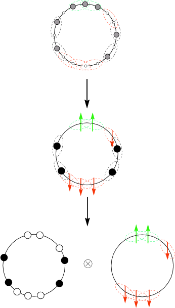
FIG. 1.: The mapping is illustrated in this Figure. In the first chain, the circles stand for occupied sites while the small dots stand for empty ones. The introduction of the nearest-neighbor interaction leads to a further factorization of the wave function describing the charge degrees of freedom.

- [1] P. W. Anderson, Science 235, 1196 (1987).
- [2] P. W. Anderson, The theory of superconductivity in the High cuprates, Princeton E.P., Princeton N.J., (1997).
- [3] F. C. Zhang and T. M. Rice, Phys. Rev. B 37,3759 (1988).
- [4] B. Dardel, D. Malterre, M. Grioni, P. Weibel, and Y. Baer, Phys. Rev. Lett. 67, 3144 (1991).
- [5] H. J. Schulz, Phys. Rev. Lett. 64, 2831 (1990).
- [6] H. Bethe, Z. Phys. 71, 205 (1931).
- [7] E. Lieb and F. Y. Wu, Phys. Rev. Lett. 20, 1445 (1965).
- [8] M. Ogata and H. Shiba, Phys. Rev. B 41, 2326 (1990).
- [9] Karlo Penc, Karen Hallberg, Fr d ric Mila, and Hiroyuki Shiba, Phys. Rev. Lett. 77, 1390 (1996).
- [10] Karlo Penc, Fr d ric Mila, and Hiroyuki Shiba, Phys. Rev. Lett. 75, 894 (1995).
- [11] H. Eskes and A. M. Olés , Phys. Rev. Lett. 73, 1279 (1994).
- [12] A. Parola and S. Sorella, Phys. Rev. Lett. 64, 1831 (1990).
- [13] R. G. Dias and J. M. Lopes dos Santos, Journal de Physique I 2, (1992) 1889.
- [14] N. M. R. Peres, R. G. Dias, P. D. Sacramento, and J. M. P. Carmelo, Phys. Rev. B (to be published 15 February 2000).
- [15] F. Gebhard, K. Bott, M. Scheidler, P. Thomas, and S. W. Koch, Philos. Mag. B, 75, 1 (1997); 75, 13 (1997); 75, 47 (1997).
- [16] P. Jordan and E. Wigner, Z. Physik 47, 631 (1928).
- [17] C. N. Yang and C. P. Yang, Phys. Rev., 150, 321 (1966); 150, 327 (1966); 151, 258 (1966).
- [18] N. M. R. Peres, P. D. Sacramento, D. K. Campbell and J. M. P. Carmelo, Phys. Rev. B 59, 7382 (1999).
- [19] B. Sutherland and B. S. Shastry, Phys. Rev. Lett. 65, 1833 (1990); 65, 243 (1990).
- [20] F. V. Kusmarstev, Phys. Lett. A 161, 433 (1992).
- [21] F. D. M. Haldane, J. Phys. C 14, 2585 (1981); Phys. Rev. Lett. 45, 1358 (1980).
- [22] G. Gomez-Santos, Phys. Rev. Lett. 70, 3780 (1993).
- [23] X. Zotos and P. Prelovšek, Phys. Rev. B 53, 983 (1996).
- [24] H. Castella, X. Zotos, and P. Prelovšek, Phys. Rev. Lett. 47, 972 (1995)
- [25] X. Zotos, F. Naef, and P. Prelovšek, Phys. Rev. B 55, 11029 (1997).
- [26] W. Khon, Phys. Rev. 133, A171 (1964).
- [27] B. S. Shastry and B. Sutherland, Phys. Rev. Lett. 65, 243 (1990).
- [28] M. Takahashi, Prog. Theor. Phys. 46, 401 (1971); M. Takahashi and M. Suzuki, Prog. Theor. Phys. 48, 2187 (1972).
- [29] M. Gaudin, Phys. Rev. Lett. 26, 1302 (1971).
- [30] S. K. Lyo and J. P. Galinar, J. Phys. C 10, 1693 (1977).
- [31] S. K. Lyo, Phys. Rev. B 18, 1854 (1978).
- [32] J. M. P. Carmelo,P. D. Sacramento, N. M. R. Peres, and D. Baeriswyl, cond-mat/9805043; J. M. P. Carmelo, N. M. R. Peres, and P. D. Sacramento, Phys. Rev. Lett. (to be published).
- [33] R. G. Dias, unpublished.