[

Nesting Induced Precursor Effects: a Renormalization Group Approach

Abstract

We develop a controlled weak coupling renormalization group (RG) approach to itinerant electrons. Within this formalism we rederive the phase diagram for two-dimensional (2D) non-nested systems. Then we study how nesting modifies this phase diagram. We show that competition between p-p and p-h channels, leads to the manifestation of unstable precursor fixed points in the RG flow. This effect should be experimentally measurable, and may be relevant for an explanation of pseudogaps in the high temperature superconductors (HTC), as a crossover phenomenon.

]

An important clue to understand the physics of the HTC may come from the unconventional normal state properties preceding superconducting ordering: a pseudogap is opened, which manifests through an apparent continuous reduction in the density of states[1] at a temperature $T^{*}$, higher than the superconducting critical temperature, $T_{c}$. The precise definition of this incipient ordering mechanism is still subject of discussion[2]^,[3]. Two main pictures have been proposed depending on whether the correlations being built up in the pseudogap are of superconducting[4] or (spin, or charge) density wave nature[5]. However no experimental conclusive proof has been given so far favoring any of these pictures.

In the former, it is assumed that pre-formed pairs appear at the pseudogap energy scale $T^{*}$, but coherence would only be established at $T_{c}.$ Some support in favor of this scenario is provided for instance by ARPES measurements. They indicate that the pseudogap shares some of the superconducting properties like the gap symmetry. Furthermore, they reveal the presence of a non-vanishing gap in the vicinity of the $\left(\pi,0\right)$ point already above $T_{c}$[6]. Nevertheless, it has been argued that NMR and heat capacity data show that superconductivity and pseudogap are competing[7], like antagonistic phases. Also, $T^{*}$ merges with $T_{c}$ at a critical doping in the overdoped superconducting region, when the condensation energy, the critical currents and the superfluid density reach sharp maxima. This has been argued to be irreconcilable with a preformed pairing scenario[2].

The amplitude of incommensurate peaks observed in inelastic neutron scattering varies upon doping in a way highly related to the pseudogap and falls to zero in the overdoped region[2]. ARPES has clearly shown the existence of a Fermi surface which is lying not too far from the diagonals of the first Brillouin zone[6], therefore providing an approximate nesting.

In the ideal case of perfect nesting, it is well known that density wave and superconducting instabilities are strongly interfering[8]^- [14]. In this work we present a simple one-loop RG approach to electrons on 2D Fermi surfaces with flat nested regions, away from half-filling. We show that the strong competition arising from particle-particle and particle-hole corrections when nesting of the Fermi surface (FS) is included, naturally induces instabilities that can be preceded by other incipient instabilities. In the RG sense this appears as a crossover phenomenon: the RG flow passes near an unstable fixed point, capturing the physics of this fixed point at intermediate energies, before the system orders in the final superconducting state. This scenario naturally provides two energy scales and therefore bears striking similarities with the pseudogap phase of the HTC’s. The condition of perfect nesting may be relaxed provided interactions are large enough.

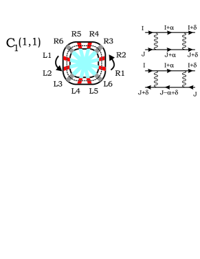
FIG. 1.: Left: Tomographic parameterisation of a Fermi surface with 3 patches per side ($N_{c}=3$): 2 on nested regions (N=2) and 1 in curved portions (M=1). The $C_{1}\left(1,1\right)$ is illustrated. Right: Diagrams considered.

We parametrize a 2D Fermi surface with a set of $4N_{c}$ patches, as illustrated in figure 1. The kinetic energy dispersion is linearized around the Fermi surface, each patch being assigned a Fermi velocity, $v_{{I}}.$ In this work all $v_{{I}}$ are assumed equal as the results do not depend significantly on smooth Fermi velocity modulations. The most general spin rotational invariant interaction term which remains in an effective low energy theory only involves incoming electrons on opposite sides of the Fermi surface[13, 15]. This remark enables us to separate the set of patches in two complementary subsets called right ($R$) and left ($L$) patches, for convenience. We may therefore write:

$${\cal H}_{C} = \frac{1}{2N_{c}L}\sum_{{I,K,\delta}}\,\sum_{q\simeq 0}\ (C_{{\delta}}^{c}({I,J})\,J_{q,{\delta}}^{R}\left({I}\right)\,J_{-q,-{\delta}}^{L}\left({K}\right)$$ (2)

$$+C_{{\delta}}^{s}({I,J})\,{\bf J}_{q,{\delta}}^{R}\left({I}\right)\cdot{\bf J}_{-q,-{\delta}}^{L}\left({K}\right))$$

where charge $J_{{\delta}}^{R}({I})=\sum_{\tau,\tau^{\prime}}:R_{{I+\delta},\tau}^{+}\;\delta_{\tau,\tau^{\prime}}\,\,R_{{I},\tau^{\prime}}:$ , and spin currents ${\bf J}_{{\bf\delta}}^{R}({I})=\sum_{\tau,\tau^{\prime}}:R_{{I+\delta},\tau}^{+}\;{\bf\sigma}_{\tau,\tau^{\prime}}\,\;R_{{I},\tau^{\prime}}:,$ have been used, and momentum variables within each patch have been omitted to simplify the notation. Here chain indices could have been written in bold as they could represent vectors[12]. In that case we could, for instance, consider a bilayer of 2D electron systems: the present formalism is in fact quite general allowing the treatment of many different systems. Eq. $\left(\ref{interaction}\right)$ allows an extremely simple derivation of one-loop equations: only the two diagrams in fig. 1, need to be considered. Requiring the invariance of the two-particle vertex under cutoff reduction we arrive at ($\partial\equiv\partial/\partial\ln D$ and $C_{i}\equiv C_{i}/2\pi N_{c}$) :

$$\partial C_{{\delta}}^{c}({I,K})\text{{}} = \text{{}}\sum_{{\alpha}}\delta^{c}({I,K,\delta,\alpha})\,{(}C_{{\alpha}}^{c}({I,K})C_{{\delta-\alpha}}^{c}({I+\alpha,K+\alpha})$$ (6)

$$+3C_{{\alpha}}^{s}({I,K})C_{{\delta-\alpha}}^{s}({I+\alpha,K+\alpha}){)/}\left(v_{{I+\alpha}}+v_{{K+\alpha}}\right)$$

$$-\sum_{{\alpha}}\delta^{ZS}({I,K,\delta,\alpha}){(}C_{{\alpha}}^{c}({I,K-\alpha+\delta})C_{{\delta-\alpha}}^{c}({I+\alpha,K})$$

$$+3C_{{\alpha}}^{s}({I,K-\alpha+\delta})\,C_{{\delta-\alpha}}^{s}({I+\alpha,K}){)/}\left(v_{{I+\alpha}}+v_{{K-\alpha+\delta}}\right)$$

for charge couplings, whereas for spin couplings we get:

$$\partial C_{{\delta}}^{s}({I,K}) = \sum_{{\alpha}}\delta^{c}({I,K,\delta,\alpha})\,{(}C_{{\alpha}}^{s}({I,K})C_{{\delta-\alpha}}^{c}({I+\alpha,K-\alpha})$$ (12)

$$+C_{{\alpha}}^{c}({I,K})C_{{\delta-\alpha}}^{s}({I+\alpha,K-\alpha})$$

$$-2C_{{\alpha}}^{s}({I,K})\,C_{{\delta-\alpha}}^{s}({I+\alpha,K-\alpha}){)}/\left(v_{{I+\alpha}}+v_{{K+\alpha}}\right)-$$

$$-\sum_{{\alpha}}\delta^{ZS}({I,K,\delta,\alpha}){(}C_{{\alpha}}^{c}({I,K-\alpha+\delta})C_{{\delta-\alpha}}^{s}({I+\alpha,K})$$

$$+C_{{\alpha}}^{s}({I,K-\alpha+\delta})C_{{\delta-\alpha}}^{c}({I+\alpha,K})$$

$$+2C_{{\alpha}}^{s}({I,K-\alpha+\delta})\,C_{{\delta-\alpha}}^{s}({I+\alpha,K}){)}/\left(v_{{I+\alpha}}+v_{{K-\alpha+\delta}}\right)$$

Here $\delta^{c}$ and $\delta^{ZS}$ implement phase space restrictions: they are equal to 1 iff all electrons involved in the scattering are kept on the FS along the process. This happens if the electrons are on nested regions of the FS, or, in the case of the Cooper channel, if ${I=K}$. Otherwise $\delta^{c}$ and $\delta^{ZS}$ are set equal to zero.

In order to characterize the possible instabilities in the system, we introduce  several response functions, of the form: ${\cal R}_{{\delta}}\left({I,K}\right)=$ $-i\int dt\,e^{i\omega t}$ $\left\langle T\left\{{\cal O}_{{\delta}}\left({I;}t\right)\,{\cal O}_{{\delta}}^{+}\left({K;}0\right)\right\}\right\rangle.$ For singlet superconductivity we denote ${\cal R}_{{\delta}}\left({I,K}\right)\equiv S_{{\delta}}^{S}\left({I,K}\right)$ and the order parameter is: ${\cal O}_{SSC,{\delta}}\left({I;}t\right)=\frac{1}{\sqrt{2}}\sum_{\tau}\tau\,R_{{I+\delta},\tau}\left(t\right)L_{{I},-\tau}\left(t\right).$ For triplet superconductivity, ${\cal R}_{{\delta}}\left({I,K}\right)\equiv S_{{\delta}}^{T}\left({I,K}\right),$ and ${\cal O}_{TSC,{\delta}}\left({I;}t\right)=\frac{1}{\sqrt{2}}\sum_{\tau}R_{{I+\delta},\tau}\left(t\right)L_{{I},-\tau}\left(t\right).$ As interactions do not connect pairs of particles with different ${\delta}$ (because of momentum conservation)[13], the problem of finding the most divergent instabilities is reduced to that of diagonalizing matrices $S_{{\delta}}\left({I,K}\right),$ with ${\delta}$ fixed. The eigenvectors determine the order parameter characterizing the instability.

For charge density wave we define ${\cal R}_{{\delta}}\left({I,K}\right)\equiv D_{{\delta}}^{c}\left({I,K}\right),$ with the order parameter ${\cal O}_{CDW,{\delta}}\left({I}\right)=\frac{1}{\sqrt{2}}\sum_{\tau}\,R_{{I+\delta},\tau}^{+}\,L_{{I},\tau}\,$  $\equiv\frac{1}{\sqrt{2}}\sum_{\tau}\,R_{{M+Q},\tau}^{+}\,L_{{M-Q},\tau}\;$(i.e., ${M=I+}\frac{{\delta}}{2}$ and $\,{Q=}\frac{{\delta}}{2}$). The last definition stresses that interactions connect only order parameters with equal particle-hole center of mass, ${M.}$ Thus, the problem of diagonalizing $D_{{\delta}}^{c}\left({I,K}\right)$ is once again simplified as there is a fixed parameter. Finally for spin density waves we define similarly ${\cal O}_{SDW,{\delta}}\left({I}\right)=$ $\frac{1}{\sqrt{2}}\sum_{\tau}\,\tau\,R_{{M+Q},\tau}^{+}\,L_{{M-Q},\tau}.$

With these definitions it is straightforward to obtain RG equations for the response functions[8]^,[13], of the form $\partial\ln\overline{{\cal R}}_{{\delta}}\left({I,K}\right)/\partial\ln D=\upsilon$ with $\overline{{\cal R}}_{{\delta}}\left({I,K}\right)$= $\pi\left(v_{{I}+{\delta}}+v_{{I}}\right)\partial{\cal R}_{{\delta}}\left({I,K}\right)/\partial\ln\omega$. More precisely:

$$\upsilon_{SSC} = -\frac{C_{{I-K}}^{c}\left({K},{K}+{\delta}\right)-3C_{{I-K}}^{s}\left({K},{K}+{\delta}\right)}{\left(v_{{K}+{\delta}}+v_{{K}}\right)}$$ (13)

$$\upsilon_{TSC} = -\frac{C_{{I-K}}^{c}\left({K},{K}+{\delta}\right)+C_{{I-K}}^{s}\left({K},{K}+{\delta}\right)}{\left(v_{{K}+{\delta}}+v_{{K}}\right)}$$ (14)

$$\upsilon_{CDW} = \frac{C_{{I-K}}^{c}\left({K,I+\delta}\right)+3C_{{I-K}}^{s}\left({K,I+\delta}\right)}{\left(v_{{2I-K+\delta}}+v_{{K}}\right)}$$ (15)

$$\upsilon_{SDW} = \frac{C_{{I-K}}^{c}\left({K,I+\delta}\right)-C_{{I-K}}^{s}\left({K,I+\delta}\right)\,\,}{\left(v_{{2I-K+\delta}}+v_{{K}}\right)}$$ (16)

In this work we are concerned with the ordering of the electronic system. As a general trend, the effective couplings in the one-loop approximation diverge for a finite value of the reduced cut-off. This is naturally interpreted as the signature of a low temperature instability towards an ordered state. However this divergency of the effective couplings also signals a breakdown of the one-loop approximation. This difficulty may be overcome by noting that in general ratios of any two coupling constants reach finite asymptotic values as the instability is approached[14]. In this work we have thus emphasized the study of these asymptotic flows in the space of directions for the effective coupling vector. Representing the $C_{{\delta}}({I,J})$ by a generic $C_{i},$ this can be done by finding the flow of non-diverging normalized couplings $c_{i}\equiv C_{i}/{\cal N},$ with ${\cal N=}\sqrt{\sum_{j}\left(C_{j}\right)^{2}}$ (the sum is over all the couplings). From the RG equations $\left(\ref{RG1}\right)$ and $\left(\ref{RG2}\right)$ having the form $\partial C_{i}/\partial\ln D=$ $A_{ijk}\,C_{j}C_{k}$ we obtain the evolution for the normalized couplings: $dc_{i}/du=\sum_{jkl}A_{jkl}\,c_{k}$ $c_{l}\left(\delta_{ij}-c_{i}c_{j}\right).$ We have introduced a new scale parameter $u$ related to $D$ by $du=-{\cal N}$ $d\ln D$. In this parametrization the magnitude ${\cal N}$ of the coupling vector diverges only as $u\rightarrow\infty.$ From the flow as a function of $u$, we can recover the more physical variable $D$ since $d\ln{\cal N}/du$= $A_{ikl}\,c_{i}\,c_{k}\,c_{l}$ which yields ${\cal N}\left(u\right)$ and therefore $D\left(u\right)$. A similar procedure can be applied to the computation of response functions, that we generically represent by $\overline{{\cal R}}_{i}$. Their RG equations have the form $d\ln\overline{{\cal R}}_{i}/d\ln D=B_{ik}\,C_{k}$, which becomes $d\ln\overline{{\cal R}}_{i}/du=B_{ik}\,c_{k}$. As $u$ goes to infinity the r.h.s. reaches a finite value. This is easily seen to imply a divergency of the form ${\cal R}_{i}\sim[\,\ln(D/D^{*})\,]^{-\alpha_{i}}$, where $D^{*}$ is the scale at which the instability occurs. The exponents $\alpha_{i}$ are completely determined by the fixed point values $c_{i}^{*}$ of the normalized couplings.

This procedure provides a controlled framework to study the complete RG flow (not restricted to the one-loop approximation) provided the bare couplings are small enough. Certainly we expect the one-loop approach to break down if ${\cal N}$ is of the order unity. For a given choice of initial couplings with norm ${\cal N}_{0}$, this yields a maximal value of $u$ ($u_{\max}$) beyond which our approximation is no longer reliable. The main point is that $u_{\max}$ can be made arbitrarily large provided ${\cal N}_{0}\,$is small enough. In general we expect $u_{\max}\sim\ln(1/{\cal N}_{0})$. In some applications we are also interested in a finite an not infinitesimal ${\cal N}_{0}$ regime. Higher order corrections destroy the fixed directions found in the one-loop approximation. However, we conjecture those become fixed points in the usual sense and that the topology of the one-loop flow pattern is preserved.

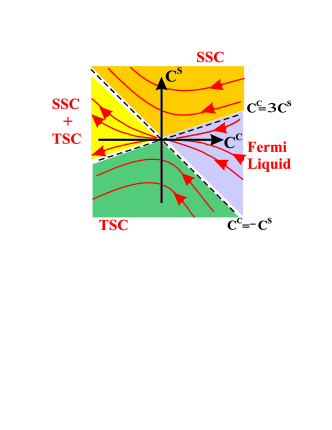
FIG. 2.: Phase diagram for a two dimensional isotropic electronic system with a circular Fermi surface.

As a first example of application of the present formalism we consider a non-nested Fermi surface. The spinless case is thoroughly discussed in the review paper by Shankar[15]. Phase space restrictions set in $\left(\ref{RG1}\text{-}\ref{RG2}\right)$ through the $\delta$ functions, imply that only couplings of the form $C_{{\delta}}({I,I})$ are renormalized, due to particle-particle corrections (BCS channel). Divergence of the flow is then related to superconductivity. Indeed, inspired from (13-14), the RG flow equations can be quite simply written in terms of singlet $C_{{\delta}}^{S}({I})\equiv C_{{\delta}}^{c}({I,I})-3C_{{\delta}}^{s}({I,I})$ and triplet couplings$\,C_{{\delta}}^{T}({I})\equiv C_{{\delta}}^{c}({I,I})+C_{{\delta}}^{s}({I,I})$:

$$\partial C_{{\delta}}^{T}({I})=\alpha\left(C_{{\delta}}^{T}({I})\right)^{2}\;\;\;\;\;\;\partial C_{{\delta}}^{S}({I})=\alpha\left(C_{{\delta}}^{S}({I})\right)^{2}$$ (17)

where $\alpha$ is a Fermi velocity dependent constant. The phase diagram is shown in Figure 2, for a system with initial couplings $C_{{\delta}}^{c}({I,I})=C^{c}$ and $C_{{\delta}}^{s}({I,I})=C^{s}$. The only region where the flow does not diverge corresponds to a Fermi Liquid phase[15]. In the other regions, the RG couplings diverge at the energy scale that we associate with the superconducting critical temperature, $T_{c}$.

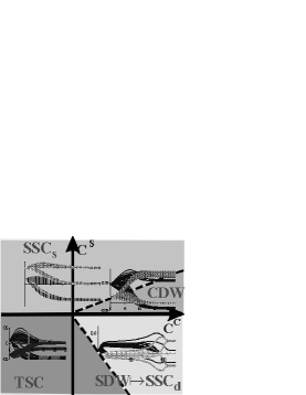
FIG. 3.: Phase diagram for a nested system: the flows of the couplings in each phase are inserted.

This picture changes when we introduce nesting. As already discussed [10, 12] flat regions dramatically enhance the number of low energy couplings to be considered. The occurrence of log singularities in both the particle-particle and the particle-hole channels induce an intricate interference mechanism, leading to the so-called parquet regime. In Figure 3, we show the new phase diagram, together with typical flow patterns (using the $u$ variable, and normalized couplings) for each of the different phases. These results have been obtained for a partially nested Fermi surface with $N=6$ patches along each flat segment and $M=0$ along each curved arc. Note that increasing the number of patches doesn’t change significantly the phase-diagram.

The modifications due to nesting are most obvious in the initial coupling domain corresponding to the Fermi liquid regime for the circular Fermi surface. For positive bare spin coupling, we obtain a CDW phase, as a mean field analysis predicts. The most striking result appears for repulsive couplings in the charge sector and moderate negative spin couplings. With this parametrization, the simple repulsive Hubbard model falls in this region. The flow pattern from Figure 3 clearly shows a two-step evolution as $u$ is increased. Before entering the final asymptotic regime, the system spends a large $u$-time in the proximity of an unstable fixed point (for the normalized couplings). In this intermediate phase, the most diverging response is the SDW susceptibility. The corresponding order parameter has the approximate form $R^{+}_{N}L_{1}+R^{+}_{N-1}L_{2}+...+h.c$ so the most favorable nesting vector is perpendicular to the flat regions. Couplings involving incoming and outgoing electrons close to the endpoints of flat regions are the most enhanced. This intermediate fixed point corresponds very likely to the one found by Zheleznyak et al [10] who worked with the original un-normalized couplings. Our approach yields the remarkable result that the system is finally attracted towards a stable low energy d-wave superconductor ($SSC_{d}$) fixed point. Again, the largest couplings involve the endpoints of the flat regions, and from the superconducting response function, the gap exhibits a strong anisotropy. It vanishes at the center of flat regions and reaches its maximal values at their extremities. The dramatic role played by these extremal regions suggests some similarity with the Van-Hove singularity scenario studied by several groups [9, 11, 16]. However, we haven’t introduced any singularity in the Fermi velocity. Our model also ignores Umklapp processes, which are expected to play a crucial role in stabilizing a commensurate SDW (Néel state), and in describing the proximity to a Mott insulator [11].

It is important to specify the energy scales associated to both fixed points. Assuming the bare bandwidth is $D_{0}$, the correspondence between the running scale $D$ and the fictitious time $u$ takes the form: $ln(D_{0}/D)=h(u)/{\cal N}_{0}$, where ${\cal N}_{0}$ is the length of the initial coupling vector, and $h(u)$ is a function depending on the direction of this vector. In general, $h$ appears to be an increasing function of $u$ which reaches a finite limit $h(\infty)$ as $u$ becomes infinite. This defines the instability scale $D_{c}$ below which the system is superconducting. Similarly, we define a scale $D_{1}$ for which the distance of the normalized coupling vector to the intermediate fixed point is minimal. Let us note by $u_{1}$ the corresponding value of $u$. We obtain: $D_{1}/D_{0}=(D_{c}/D_{0})^{h(u_{1})/h({\infty})}$, which holds for a chosen direction of the initial coupling vector. $D_{c}$ and $D_{1}$ are considered here to be functions of ${\cal N}_{0}$. In practice, we have found that $h(u_{1})/h({\infty})$ is very close to unity. As an order of magnitude, if $D_{c}\simeq 100K$ and $D_{0}\simeq 5000K$, $D_{1}-D_{c}\simeq 1K$. However, SDW correlations begin to build up at a much higher energy scale, as can be seen in Figure 4. We may for instance evaluate the scale $D^{*}$ at which the SDW exponent reaches 99 percent of its maximal value.

$N$	$3\ \ \$	$6\ \$	$8\ \$	$\ \ \ 10\ \ \ \$	$\ \ \ 12\ \ \$	$14\$
$T_{c}\left(K\right)$	$0$	$0.0$	$0.2$	$15$	$82$	$150$
$T^{*}\left(K\right)$	$0$	$0.0$	$9$	$208$	$736$	$1066$
Table 1: System with N+M=14 and normalized couplings.

From the table above, we conclude that there can be a large temperature range for which a SDW enhancement is observed above the superconducting instability. Both temperature scales are seen to decrease as the length of nested segments is reduced. This reduction is accompanied by an increase in the minimal distance to the unstable fixed point along the flow. This leads to a less pronounced intermediate regime, smaller exponents for the SDW response, and consequently a smaller magnitude of SDW correlations.

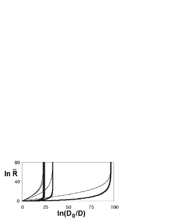
FIG. 4.: Flow of the dominant SDW (thin) and SSCd (thick) response functions for systems with N+M=14, but different nesting qualities (N=14,12,8,3). Better nested systems develop instabilities at higher energy scales. SSCd response functions become the most diverging responses at the final energy scale, associated with $T_{c}$.

In summary, we have shown that precursor effects are predicted by a controlled weak coupling RG approach to fermionic systems. The flow approaches an unstable fixed point for systems with repulsive interactions, before being attracted to the final stable superconducting fixed point controlling the low temperature physics of the system. SDW response functions are enhanced and dominate near the intermediate fixed point, before the d-wave superconducting response finally diverges. We believe that Umklapp processes are likely to strengthen this picture. Close to half-filling, they are not expected to compete with SDW ordering, but with superconductivity, thereby reducing $T_{c}$ without affecting the cross-over energy scale. In spite of the weak coupling limit chosen here, we observe striking similarities with the pseudogap behavior of the HTC. This suggests that the strength of interactions in real materials may compensate the deviations of the observed Fermi surface from perfect nesting.

The authors acknowledge discussions with D. Zanchi, K. Le Hur and R. Dias. This work received traveling support from ICCTI/CNRS, Proc.423. FVA also benefited from the MCT Praxis XXI Grant No. 2/2.1/Fis/302/94.

REFERENCES

- [1] C.C. Homes et al, Phys. Rev. Lett. 71, 1645 (1993); H. Ding et al, Nature 382, 51 (1996); A.G. Loeser et al, Science 273, 325 (1996).
- [2] J.L. Tallon and J.W. Loram, cond-mat/0005063
- [3] T. Timusk and B. Statt, Rep. Prog. Phys. 62, 61 (1999)
- [4] Jan R. Engelbrecht et al, Phys. Rev. Lett. 57, 13406 (1998); P. Nozières and S. Schmitt-Rink, J. Low Temp. Phys. 59, 195 (1985); V.J. Emery and S.A. Kivelson, Phys. Rev. Lett. 64, 475 (1990)
- [5] T. Tanamoto, H. Kohno and H. Fukuyama, J. Phys. Soc. Jpn 63, 2739 (1994); J. Schmalian, D. Pines and B. Stojkovic, Phys. Rev. Lett. 80, 3839 (1998)
- [6] H. Ding et al, Phys. Rev. Lett. 78, 2628 (1997); P.V. Bogdanovet al, cond-mat/0005394; Borisenko et al,Phys. Rev. Lett. 84, 4453 (2000); .
- [7] J.W. Loram et al, Physica C 235-240, 134 (1994); J.L. Tallon and G.V.M. Williams, Phys. Rev. Lett. 82, 3725 (1999).
- [8] J. Solyom, Adv. Phys. 28, 201 (1979).
- [9] D. Zanchi and H.J. Schulz, Phys.Rev. B 61, 13609 (2000), C.J. Halboth and W. Metzner, Phys.Rev. B 61, 7364 (2000)
- [10] A.T. Zheleznyak, V.M. Yakovenko, I.E. Dzyaloshinskii, Phys. Rev.B 55, 3200 (1997)
- [11] C. Honerkamp et al, cond-mat/9912358
- [12] F. Vistulo de Abreu and B. Doucot, Europhys. Lett. 38, 533 (1997); F. Vistulo de Abreu, PhD Thesis, UJF, Grenoble (1997), (unpublished).
- [13] B. Douçot and F. Vistulo de Abreu, to be published.
- [14] L. Balents and M.P.A. Fisher, Phys. Rev. B 53, 12133 (1996)
- [15] R. Shankar, Rev. Mod. Phys. 66, 129 (1994).
- [16] J. Gonzalez, F. Guinea, M.A.H. Vozmediano, Phys. Rev. Lett. 84, 4930 (2000)