Small world effects in evolution

Abstract

For asexual organisms point mutations correspond to local displacements in the genotypic space, while other genotypic rearrangements represent long-range jumps. We investigate the spreading properties of an initially homogeneous population in a flat fitness landscape, and the equilibrium properties on a smooth fitness landscape. We show that a small-world effect is present: even a small fraction of quenched long-range jumps makes the results indistinguishable from those obtained by assuming all mutations equiprobable. Moreover, we find that the equilibrium distribution is a Boltzmann one, in which the fitness plays the role of an energy, and mutations that of a temperature.

I Introduction

Darwinian evolution on asexual organisms acts by two mechanisms: mutations, that increase the genetic diversity, and selection, that fixes and reduces this diversity.

We classify mutations into point ones, corresponding to local displacements on the genotypic space (defined more accurately in the following), and other type of mutations or rearrangements, which imply larger jumps. Mutations are quite rare, so we can safely assume that for each generation at most only one mutation occurs. From a biological point of view, this discussion applies to unicellular asexual organisms, for which there is no distinction between somatic and germ cells. Moreover, we do not consider the possibility of recombination (exchange of genetic material). For non-recombinant (asexual) organisms, the combined effects of reproduction and mutations correspond to a random walk on the genotypic space. Even sexual (recombinant) populations do transmit asexually some part of their genotype, such as mithocondrial or y-chromosome DNA, to which the following analysis applies. Furthermore, we assume a constant environment.

We schematize the effects of selection by the selective reduction of the survival probability. Selection results from several constraints and can affect the frequency of certain genotypes, or even eliminate them from the population. We classify the components of selection into static and dynamic ones. In the first class we put the constraints that are independent on the population distribution, such as the functionality of a certain protein or the tuning of a metabolic path. The static part of the selection is equivalent to the concept of “fitness landscape” [1, 2]. The dynamic part of the selection originates from to the competition among individuals. We assume in this schematization that the competition only arises because the population shares some external resource which is evenly distributed, i.e. we disregard the effects of the inter-individual competition [3, 4]. In this limit the effects of competition do not depend on the distribution of genotypes, and simply limit the total size of the population.

The most important effects of the selection can be roughly schematized by assuming that certain genotypes are forbidden, so that they are eliminated from the accessible space. Let us consider for the moment that evolution takes place in a flat fitness landscape. In this frame, there are no interactions among individuals: the evolution is given by the simple superposition of all possible lineages. The probability distribution of the population in the genotypic space at a given time can be obtained by summing over all possible individual “histories” in a way similar to the path integral formulation of statistical mechanics [5]. In this view, the phylogenetic lineage of an individual is given by the path connecting the genotypes of ancestors.

This assumption has to fail somewhere, since otherwise evolution would be equivalent to a diffusion process, without anything favoring the formation of species. It often assumed that speciation events are rare and occur in a very short time [6], either due to some change in the fitness landscape (caused by an external catastrophes like the fall of a large meteorite, or by an internal rearrangement induced by coevolution) or because small isolated populations, escaping from competition, are free to explore their genotypic space (genetic drift) and find a path to an higher fitness peak [7]. Therefore, it is usually assumed that one can reconstruct the diverging time of two species from their genotypic distance from a single speciation event [8].

It is however known from recent investigations about the small-world phenomenon [9], that diffusion is seriously affected even by a small fraction of long-range jumps [10]. This fact could have dramatic consequences in our understanding of the large-scale evolution mechanism. If the short-range mutations are dominant, the evolution is equivalent to a diffusion process in the genotypic space. Assuming that the fitness landscape is formed by mountains separated by valleys, and that the crests of mountains are almost flat, then the large-scale evolution is dominated by the times needed to cross a valley by chance, while the short-scale is dominated by the neutral exploration of crests [6, 11].

Vice versa, if the long-range mutations are important (eventually amplified by the small-world mechanism), the time needed to connect two genotypes does not depend on their distance nor by the shape of the fitness landscape and the fitness maxima are quickly populated. Moreover, in this scenario, the speciation phenomenon should not be ascribed to the “discovery” of a preexisting niche, but rather to the formation of that niche in a given ecosystem due to internal interactions (coevolution) or external physical changes (catastrophes). After the formation, the niche is quickly populated because of the long-range mutations. In this framework, allopatric speciation [7] looses its fundamental importance, and sympatric speciation due to coevolution [12, 13] becomes a plausible alternative.

In order to evaluate quantitatively the relevance of these speculations, we introduce an individual-based model of an evolving population. We assume that the genetic information (the genotype) of an individual is represented by a binary string $\boldsymbol{x}=(x_{1},x_{2},\dots,x_{L})$ of $L$ symbols $x_{i}=0,1$ (multilocus model with two alleles). In this way we are modeling haploid organisms, i.e.  bacteria or viruses or, more appropriately, more archaic, pre-biotic entities. The choice of a binary code is not fundamental but certainly makes things easier. It can be justified by thinking at a purine-pyrimidine coding, or to “good” and “bad” alleles for genes (units of genetic information). In this second version, $0$ represents a good gene and $1$ a bad one. This is a sort of “minimal model” which is often used to model the evolution of genetic populations [12, 13, 14, 15, 16]. For bacteria, one can give indications that major and minor codons work in such a way [17]. The genotypic space is thus a Boolean hypercube of $L$ dimensions, and each individuals sits on a corner of this cube, according to its genotype. The $2^{L}$ corners of this hypercube represent all possible genotypes, which are at a maximum distance equal to $L$.

In the next section, we formalize the model and introduce the mathematical representation of mutation mechanisms. Then, in Section III, we consider the consequences of short and long-range mutations for a flat fitness landscape. In the long-range case all genotypes are connected, regardless of their mutual distance: this case can be considered the equivalent of a mean-field approximation. We derive analytically the rate of spreading $v$ and the characteristic spreading time $\tau$ of a genetically homogeneous inoculum in the short-range ($v_{s}$, $\tau_{s}$) and long-range ($v_{\ell}$, $\tau_{\ell}$) cases. In the first case, $v_{s}$ is independent of the genotype length $L$, and $\tau_{s}$ grows linearly with $L$; the opposite happens in the long-range case. Clearly, this different behavior has dramatic evolutionary consequences as $L$ becomes large.

In general, however, only a small set of all possible long-range mutations is observed in real organisms. We thus compute numerically the rate of spreading $v$ in a mixed short-range and sparse long-range case. A small-world effect can be observed: in the limit of large genotype lengths, a vanishing fraction of long-range mutations cooperates with the short-range ones to give essentially the mean-field results.

In Section IV, we show that the effects of mutations and selection can be separated in the limit of a very smooth fitness landscape and mean-field long-range mutations. In this approximation we obtain analytically that the asymptotic probability distribution is a Boltzmann equilibrium one, in which the fitness plays the role of of an energy and mutations correspond to temperature. We compute numerically the asymptotic probability distribution for several fitness landscapes, finding that the equilibrium hypothesis is verified. As a nontrivial example of small-world effects in evolution, we checked numerically that this scenario still holds for a sparse long-range mutation matrix. Conclusions and perspectives are drawn in the last section.

II The model

In order to be specific, let us assume that the genotype of an individual is represented by a Boolean string of length $L$. In this way, the genotypic space is a Boolean hypercube with $2^{L}$ nodes.

The genotype of an individual is represented by a string $\boldsymbol{x}=(x_{1},x_{2},\dots,x_{L})$ of $L$ Boolean symbols $x_{i}=0,1$. Each position corresponds to a locus whose gene has two allelic forms. In this way we are modeling haploid (only one copy of each gene) organisms, i.e.  bacteria or viruses or, more appropriately, more archaic, pre-biotic entities. The genotype can be also viewed as a spin configuration. In this case we use the symbol $\sigma_{i}=2x_{i}-1$.

We consider two kinds of mutations: point mutations, that interchange a $0$ with a $1$, and all other mutations that do not alter the length of the genotype (transposition and inversions). We define the distance $d(\boldsymbol{x},\boldsymbol{y})$ between two genotypes $\boldsymbol{x}$ and $\boldsymbol{y}$ as the minimal number of point mutations needed to pass from $\boldsymbol{x}$ to $\boldsymbol{y}$ (Hamming distance)

$\displaystyle d(\boldsymbol{x},\boldsymbol{y})=\sum_{i=1}^{L}(x_{i}-y_{i})^{2}.$

All possible genotypes of length $L$ are distributed on the $2^{L}$ vertices of an hypercube. A point mutation corresponds to a unit displacement on that hypercube (short-range jump).

The occurrence of point mutations in real organisms depends on the identity of the symbol and on its position on the genotype; in the present approximation, however, we assume that all point mutations are equally likely. Moreover, since the probability of observing a mutation is quite small, we impose that at most one mutation is possible in one generation. The probability to observe a point mutation from genotype $\boldsymbol{y}$ to genotype $\boldsymbol{x}$ is given by the short-range mutation matrix $M_{s}(\boldsymbol{x},\boldsymbol{y})$. By denoting with $\mu_{s}$ the probability of a point mutation per generation, we have

$$M_{s}(\boldsymbol{x},\boldsymbol{y})=\left\{\begin{array}[]{ll}1-\mu_{s}&\mbox{if $\boldsymbol{x}=\boldsymbol{y}$,}\\ \dfrac{\mu_{s}}{L}&\mbox{if $d(\boldsymbol{x},\boldsymbol{y})=1$,}\\ 0&\mbox{otherwise.}\end{array}\right.$$ (1)

Other types of mutations correspond to long-range jumps in the genotypic space. The simplest approximation consists in assuming all mutations equiprobable. Let us denote with $\mu_{\ell}$ the probability per generation of this kind of mutations. The long-range mutation matrix, $M_{\ell}(\boldsymbol{x},\boldsymbol{y})$, is defined as

$$M_{\ell}(\boldsymbol{x},\boldsymbol{y})=\left\{\begin{array}[]{ll}1-\mu_{\ell}&\mbox{if $\boldsymbol{x}=\boldsymbol{y}$,}\\ \dfrac{\mu_{\ell}}{2^{L}-1}&\mbox{otherwise.}\end{array}\right.$$ (2)

In the real world, only some kinds of mutations are actually observed. We model this fact by replacing $\boldsymbol{M}_{\ell}$ with a sparse matrix $\hat{\boldsymbol{M}}_{\ell}$. We introduce the sparseness index $s$, which is the average number of nonzero off-diagonal elements of $\hat{\boldsymbol{M}}_{\ell}$. The sum of these off-diagonal elements still gives $\mu_{\ell}$. In this case $\hat{\boldsymbol{M}}_{\ell}$ is a quenched sparse matrix, and $\boldsymbol{M}_{\ell}$ can be considered the average of the annealed version.

After considering both types of mutations, the overall mutation matrix is $\boldsymbol{M}=\boldsymbol{M}_{\ell}\boldsymbol{M}_{s}$ or $\boldsymbol{M}=\hat{\boldsymbol{M}}_{\ell}\boldsymbol{M}_{s}$ for the quenched version.

We model our population at the level of the probability distribution of genotypes $\boldsymbol{p}\equiv\boldsymbol{p}(t)$, thus disregarding spatial effects. The evolution equation for $\boldsymbol{p}$ is

$$p^{\prime}(\boldsymbol{x})=\dfrac{A(\boldsymbol{x})\sum_{\boldsymbol{y}}M(\boldsymbol{x},\boldsymbol{y})p(\boldsymbol{y})}{\overline{A}},$$ (3)

where the selection function $A(\boldsymbol{x})$ corresponds to the average reproduction rate of individuals with genotype $\boldsymbol{x}$, and ${\overline{A}}=\sum_{\boldsymbol{x}}A(\boldsymbol{x})p(\boldsymbol{x})$ is the average reproduction rate of the population [1, 2, 18, 19]. We write $A(\boldsymbol{x})$ in an exponential form $A(\boldsymbol{x})=\exp(V(\boldsymbol{x}))$, and we denote $V(\boldsymbol{x})$ with the term fitness landscape.

The selection does not act directly on the genotype, but rather on the phenotype (how an individual appears to others). The phenotype of a given genotype can be interpreted as an array of morphological characteristics. We consider the simplest case, in which the phenotype if univocally determined by the genotype $\boldsymbol{x}$, which is not the general case, since polymorphism or age dependence are usually present. The general mapping between genotype and phenotype is largely unknown and is expected to be quite complex. The effects of some genes are additive (non-epistatic), while others can interact in a simple (control genes) or complex (morphologic genes) way.

A possible way of approximating these effects is to use the following form for the fitness $V(\boldsymbol{x})$:

$$V(\boldsymbol{x})=\dfrac{{\mathcal{H}}}{L}\sum_{i=1}^{L}\sigma_{i}+\dfrac{{\mathcal{J}}}{L-1}\sum_{i=1}^{L-1}\sigma_{i}\sigma_{i+1}+{\mathcal{K}}\eta(\boldsymbol{x}),$$ (4)

where $\eta(\boldsymbol{x})$ is a random function of $\boldsymbol{x}$, uniformly distributed between $-1$ and $1$ ($\langle\eta(\boldsymbol{x})\eta(\boldsymbol{y})\rangle=\delta_{\boldsymbol{x}\boldsymbol{y}}$). The “field” term ${\mathcal{H}}$ represents a non-epistatic contribution to the fitness, in which all genes have equal weight. The “ferromagnetic” term ${\mathcal{J}}$ represents simple interactions between pairs of genes (even though in general those are not symmetric) and corresponds to a weakly rough landscape. Finally, ${\mathcal{K}}$ modulates a widely rough landscape and can be thought as an approximation of the effects of complex (spin-glass like) interactions among genes.

III Spreading and small-world effects on a flat fitness landscape

In this section we study the case of a flat fitness landscape (no selection), i.e. ${\mathcal{H}}={\mathcal{J}}={\mathcal{K}}=0$. In this way we are modeling the evolution on the crest of a mountain, assuming that all deleterious mutations are immediately lethal (the part of genotype that can originate this kind of mutations is not considered), and that we can neglect the small variation of fitness along the crest. This landscape is the one usually considered in the theory of neutral evolution [11]. Let us assume that this crest is colonized by a founder deme genotypically homogeneous (a delta peak in the genotypic distribution). We want to obtain the average time needed to populate the crest according with the different mutation schemes. Since the fitness landscape is flat, $\overline{A}$ is a constant.

We are interested in the behavior of $\rho(t)$, which is the average distance of the population from a given starting genotype $\boldsymbol{x}_{0}$, i.e.

$$\rho(t)=\sum_{\boldsymbol{x}}p(\boldsymbol{x},t)d(\boldsymbol{x},\boldsymbol{x}_{0}).$$ (5)

We introduce the spreading velocity $v$ as

$\displaystyle v=\left.\dfrac{\partial\rho}{\partial t}\right|_{t=0}.$

In Appendix A we obtain the spectral properties of the mutational matrices $\boldsymbol{M}_{s}$ and $\boldsymbol{M}_{\ell}$. The corresponding spreading velocities in the limit of small time interval $t$ compared to the characteristic spreading time $\tau_{s}=L/2\mu_{s}$ (short-range) and $\tau_{\ell}=1/\mu_{\ell}$ (long-range) are $v_{s}=\mu_{s}$, Eq. (12), and $v_{\ell}=L\mu_{\ell}/2$, Eq. (13). If short and long-range mutations coexists, one has $v=v_{s}+v_{\ell}$, Eq. (14).

One can approximate the behavior of real biological systems by considering a mixture of short-range mutations, which occur with a relatively high frequency, and sparse long-range mutations, with sparseness index $s$.

We investigated the sparse case by numerical simulations, for some genotype lengths $L$. As shown in Figure 1, as soon as the sparseness index $s>0$, the numerical value of $v$ becomes very close to the mean-field one, Eq. (14). Notice that the average distance from inoculum, $\rho(t)$, is rather insensitive to the distribution of $\boldsymbol{p}$. The actual distribution can be quite different from the one obtained with the mean-field matrix $\boldsymbol{M}_{\ell}$.

This transition may be interpreted as an indication of a small-world effect, and that there exists a first-order transition at $s=0$ [20]. However, the fluctuations of the velocity, $\text{Var}(v)$, appears to diverge at $s=0$ with an exponent $1$, as shown in Figure 2.

These results suggest the presence of a small-world phenomenon in evolution: the rare and sparse long-range mutations cooperate synergetically with the short-range ones to give essentially a mean-field effect. We checked that the previous results hold also for a non-flat (but smooth) fitness landscape ($\mu_{s}=10^{-5}$, $\mu_{\ell}=10^{-4}$ and ${\mathcal{H}}=10^{-4}$, ${\mathcal{J}}=0$, ${\mathcal{K}}=0$). Again, as soon as $s>0$, the spreading velocity increases from the short-range values to the mean-field ones.

IV Equilibrium properties and small-world effects on a smooth fitness landscapes

In the following we shall study the effects of the cooperation between short-range and sparse long-range mutations on the equilibrium properties of the model.

Let us study the model in the presence of a smooth static fitness landscape. In this case the fitness $A$ does not depend explicitly on the distribution $\boldsymbol{p}$, and Eq. (3) can be linearized by using unnormalized variables $z(\boldsymbol{x},t)$ satisfying

$$z(\boldsymbol{x},t+1)=\sum_{\boldsymbol{y}}A(\boldsymbol{y})M(\boldsymbol{x},\boldsymbol{y})z(\boldsymbol{y},t),$$ (6)

with the correspondence

$\displaystyle p(\boldsymbol{x},t)=\dfrac{z(\boldsymbol{x},t)}{\sum_{\boldsymbol{y}}z(\boldsymbol{y},t)}.$

In vectorial terms, Eq. (6) can be written as

$$\boldsymbol{z}(t+1)=\boldsymbol{M}\boldsymbol{A}\boldsymbol{z}(t),$$ (7)

where $\boldsymbol{M}_{\boldsymbol{xy}}=M(\boldsymbol{x},\boldsymbol{y})$ and $\boldsymbol{A}_{\boldsymbol{xy}}=A(\boldsymbol{x})\delta_{\boldsymbol{xy}}$.

When one takes into consideration only point mutations ($\boldsymbol{M}\equiv\boldsymbol{M}_{s}$), Eq. (6) can be read as the transfer matrix of a two-dimensional Ising model [21, 22, 23], for which the genotypic element $\sigma_{i}(t)$ corresponds to the spin in row $t$ and column $i$, and $z(\boldsymbol{\sigma},t)$ is the restricted partition function of row $t$. The effective Hamiltonian ${\mathcal{V}}$ (up to constant terms) of a possible genealogical history $\{\boldsymbol{x}(t)\}$ or $\{\boldsymbol{\sigma}(t)\}$ from time $1\leq t\leq T$ is

$${\mathcal{V}}=\sum_{t=1}^{T-1}\left(\gamma\sum_{i=1}^{L}\sigma_{i}(t)\sigma_{i}(t+1)+V\bigl{(}\boldsymbol{x}(t)\bigr{)}\right),$$ (8)

where $\gamma=-\ln(\mu_{s}/(1-\mu_{s}))$.

This peculiar two-dimensional Ising model has a long-range coupling along the row (depending on the choice of the fitness function) and a ferromagnetic coupling along the time direction (for small short range mutation probability). In order to obtain the statistical properties of the system one has to sum over all possible configurations (stories), eventually selecting the right boundary conditions at time $t=1$. The bulk properties of Eq. (8) cannot be reduced in general to the equilibrium distribution of a one dimensional system, since the transition probabilities among rows do not obey detailed balance. Moreover, the temperature-dependent Hamiltonian (8) does not allow an easy identification between energy and selection, and temperature and mutation, what is naively expected by the biological analogy with an adaptive walk.

A Long-range mutations

Let us first consider the long-range mutation case. Eq. (7), reformulated according to Eq. (3), corresponds to

$\displaystyle\boldsymbol{z}(t+\tau)=(\boldsymbol{A}\boldsymbol{M}_{\ell})^{\tau}\boldsymbol{z}(t).$

Since it is easier to consider the effects of $\boldsymbol{A}$ and $\boldsymbol{M}_{\ell}$ separately, let us study in which limit they commute. The norm of the commutator on the asymptotic probability distribution $\boldsymbol{p}$ is

$\displaystyle||[\boldsymbol{A}\boldsymbol{M}_{\ell}]||=\sum_{\boldsymbol{xy}}|[\boldsymbol{A}\boldsymbol{M}_{\ell}]_{\boldsymbol{xy}}p(\boldsymbol{y})|,$

and it is bounded by $\mu_{\ell}c$, where $c=\max_{\boldsymbol{xy}}|A_{\boldsymbol{xx}}-A_{\boldsymbol{yy}}|$. In the limit $\mu_{\ell}c\rightarrow 0$ (i.e. a very smooth landscape), to first order in $c$ we have

$\displaystyle(\boldsymbol{A}\boldsymbol{M}_{\ell})^{\tau}=\boldsymbol{A}^{\tau}\boldsymbol{M}_{\ell}^{\tau}+O(\tau^{2}\mu_{\ell}c)\boldsymbol{A}^{\tau-1}\boldsymbol{M}_{\ell}^{\tau-1},$

which is the analogous of the Trotter product formula.

When $\tau$ is order $1/\mu_{\ell}$, $\boldsymbol{M}_{\ell}^{\tau}$ is a constant matrix with elements equal to $1/2^{L}$, and thus $\boldsymbol{M}_{\ell}\boldsymbol{p}$ is a constant probability distribution. If $\mu_{\ell}$ is large enough, $(\boldsymbol{A}\boldsymbol{M}_{\ell})^{\tau}=\boldsymbol{A}^{\tau}\boldsymbol{M}_{\ell}^{\tau}$.

The asymptotic probability distribution $\tilde{\boldsymbol{p}}$ is thus proportional to the diagonal of $\boldsymbol{A}^{1/\mu_{\ell}}$:

$$\tilde{p}(\boldsymbol{x})=C\exp\left(\dfrac{V(\boldsymbol{x})}{\mu_{\ell}}\right)$$ (9)

i.e. a Boltzmann distribution with Hamiltonian $V(\boldsymbol{x})$ and temperature $\mu_{\ell}$. This corresponds to the naive analogy between evolution and equilibrium statistical mechanics. In other words, the genotypic distribution is equally populated if the phenotype is the same, regardless of the genotypic distance since we used long-range mutations.

We have checked numerically this hypothesis, by iterating Eq. (3) for a time $T$ large enough to be sure of having reached the asymptotic state. We plotted the logarithm of the probability distribution $\tilde{p}(\boldsymbol{x})$ versus the value of the Hamiltonian $V(\boldsymbol{x})$. We computed the slope $1/\mu_{e}$ of the linear regression. The quantity $\mu_{e}$ is the effective “temperature” of the probability distribution according to the equilibrium hypothesis.

The results for the mean-field mutation matrix $\boldsymbol{M}_{\ell}$ are shown in Figure 3. We see that the equilibrium hypothesis is well verified in the limit $\mu_{\ell}\gg c$; and that convergence is faster for a rough landscape. In all cases the effective temperature $\mu_{e}$ is close to the expected value, i.e. to the mutation rate $\mu_{\ell}$.

B Short-range mutations

The above results only hold qualitatively for pure short-range mutations as shown in Figure 4. A small dispersion of points in figure implies that the genotypes can be divided into evenly-populated groups sharing approximately the same fitness. This is always the case for the additive fitness landscape (${\mathcal{H}}$ contribution), since in this case the position of symbols in the genotype is ininfluent, and the short-range mutations are able to homogenize the distribution inside a group. This is only approximately valid for the ${\mathcal{J}}$ contributions, since in this case the fitness depends on pairs of symbols, while mutations only act on single symbols. However, as shown in Figure 4-d, the homogeneous state is reached for a sufficiently high mutation probability. Finally, the homogeneous state is never reached for the very rough landscape case (${\mathcal{H}}$ contribution), even though the linear relation is satisfied in average.

In order to obtain a quantitatively correct prediction, one has to consider that the resulting slope $\mu_{e}$ is related to the second largest eigenvalue $\lambda_{1}$ of the mutation matrix by $\mu=1-\lambda_{1}$. When the fitness only depends on the “external field” term ${\mathcal{H}}$, in the asymptotic state the short-range mutations connects group of equal fitness. This fact is reflected by the vanishing dispersion of points in Figure 4-a and 4-b.

In all cases, we expect that in the limit of a very smooth landscape, $\mu_{e}$ tends towards the limiting value $2\mu_{s}/L$ of Eq. (11). This limit is reached faster when only the ${\mathcal{H}}$ term is present. This implies that for large genotype, the effective temperature due to short-range mutations is vanishing.

In the opposite case, when the selection is strong, the application of the matrix $\boldsymbol{A}$ “rotates” the distribution $\boldsymbol{p}$ in a way which is practically random with respect to the Fourier eigenvectors of $\boldsymbol{M}_{s}$. Thus, the effective second eigenvalue of the mutation matrix is given by $1-\mu_{s}$, obtained averaging over all the eigenvalues of Eq (11). Consequently, we obtain $\mu_{e}\simeq\mu_{s}$. This limit is reached faster in the case of a strongly disordered fitness landscape, i.e. in the limit of large ${\mathcal{K}}$. When only the ${\mathcal{J}}$ term is present, one observes an intermediate case.

C Small-world effects

Let us now consider the case of a sparse long-range mutation matrix, coupled to a stronger short-range matrix, i.e. $\mu_{s}\gg\mu_{\ell}$. We performed simulations with $\mu_{s}=0.1$ and $\mu_{\ell}=0.01$, $L=6$, 8 and 10 and varying $s$. The results are summarized in Table I.

The effects of the two kinds of mutations is additive, implying that, for small $\mu_{\ell}$, the distributions are visually similar to the short-range case, Figure 4. However, as soon as $s$ is greater than a threshold $s_{c}$, the effective temperature $\mu_{e}$ increases by the expected long-range contribution, $\mu_{\ell}$. This increment is very relevant when the effect of short-range mutations are vanishing, i.e. for smooth landscapes (${\mathcal{H}}$ and ${\mathcal{J}}$ contributions) and large genotypes. The effect is less relevant in the disordered case, (${\mathcal{K}}$ contributions), since in this case the contribution to the effective temperature by the small-range mutations do not decrease with $L$.

By increasing the weigth of the sparse long-range mutations, also the probability distribution becomes similar to the long-range case, Figure 3. We performed simulations with $\mu_{s}=0.1$ and $\mu_{\ell}=0.1$, $L=6,8,10$ varying $s$. The results are shown in Table I. Notice that the value of $s_{c}$ (estimated visually from the plot of data) is rather insensitive to $L$ and the parameters of the fitness $V(\boldsymbol{x})$.

We quantified the distance between the resulted distribution and the Boltzmann one Eq. (9) through the computation of the average square difference from linear regression, $\chi^{2}$. In Figure 5 we show that $\chi^{2}$ becomes very small as soon as $s>s_{c}$, which seems to vanish with $L\rightarrow\infty$.

This implies that, for large genotypes, a vanishing fraction of long-range mutations, coupled to small-range ones, are sufficient to establish the statistical mechanics analogy of selection and mutations.

V Conclusions

We studied some simple models of asexual populations evolving on a smooth fitness landscape, in the presence of point mutations (small-range jumps in genotypic space) and other genetic rearrangements (long-range jumps).

We have computed analitically the spreading velocity of an initially homogeneous inoculum on a flat fitness landscape, for the short-range and the long-range mean-field (all mutations equiprobable) cases. Since in the real situation only a small set of the all possible mutations can occur, we have also considered the quenched version of the long-range mutation matrix. In this case we have shown that a small-world effect is present, since even a small fraction of quenched long-range jumps makes the results indistinguishable from those obtained by assuming all mutations equiprobable. These results still hold for a smooth fitness landscape.

We have investigated this issue further, studying the equilibrium properties of the system in the presence of a smooth fitness landscape. In this framework, it has been possibile to show that the equilibrium distribution is a Boltzmann one, in which the fitness plays the role of an energy, and mutations that of a temperature. We have checked numerically this result for different fitness landscapes, and a mean-field long-range mutation mechanism. As in the previous case, a small-world phenomenon appears, since similar results can be obtained using a combination of sparse long-range and short-range mutations.

Appendix: spectral properties of the mean-field mutation matrices

Both $\boldsymbol{M}_{s}$ and $\boldsymbol{M}_{\ell}$, Eqs. (1-2), are Markov matrices. Moreover, they are circular matrices, since the value of a given element does not depend on its absolute position but only on the distance from the diagonal. This means that their spectrum is real, and that the largest eigenvalue is $\lambda_{\boldsymbol{0}}=1$. Since the matrices are irreducible, the corresponding eigenvector $\boldsymbol{\xi}_{\boldsymbol{0}}$ is non-degenerate, and corresponds to the flat distribution $\xi_{\boldsymbol{0}}(\boldsymbol{x})=1/2^{L}$. In analogy with circular matrices in the usual space, one can obtain their complete spectrum using the analogous of Fourier transform in a Boolean hyper-cubic space. Let us define the “Boolean scalar product” $\odot$:

$\displaystyle\boldsymbol{x}\odot\boldsymbol{y}=\bigoplus_{i=1}^{L}x_{i}y_{i},$

where the symbol $\oplus$ represent the sum modulus two (XOR) and the multiplication can be substituted by an AND (which has the same effect on Boolean quantities). This scalar product is obviously distributive with respect to the XOR:

$\displaystyle(\boldsymbol{x}\oplus\boldsymbol{y})\odot\boldsymbol{z}=(\boldsymbol{x}\odot\boldsymbol{z})\oplus(\boldsymbol{y}\odot\boldsymbol{z}).$

Note that the operation $\boldsymbol{x}\oplus\boldsymbol{y}$ is performed bitwise between the two genotypes: $(\boldsymbol{x}\oplus\boldsymbol{y})_{i}=x_{i}\oplus y_{i}$.

Given a function $f(\boldsymbol{x})$ of a Boolean quantity $\boldsymbol{x}\in\{0,1\}^{L}$, its “Boolean Fourier transform” is $\tilde{f}(\boldsymbol{k})$ ($\boldsymbol{k}\in\{0,1\}^{L}$)

$\displaystyle\tilde{f}(\boldsymbol{k})=\dfrac{1}{2^{L}}\sum_{\boldsymbol{x}}(-1)^{\boldsymbol{x}\odot\boldsymbol{k}}f(\boldsymbol{x}).$

The anti-transformation operation is determined by the definition of the Kronecker delta

$\displaystyle\delta_{\boldsymbol{k}\boldsymbol{0}}=\dfrac{1}{2^{L}}\sum_{\boldsymbol{x}}(-1)^{\boldsymbol{x}\odot\boldsymbol{k}},$

and is given by

$\displaystyle f(\boldsymbol{x})=\sum_{\boldsymbol{k}}(-1)^{\boldsymbol{x}\odot\boldsymbol{k}}\tilde{f}(\boldsymbol{k}).$

One can easily verify that the Fourier vectors $\xi_{k}(\boldsymbol{x})=(-1)^{\boldsymbol{x}\odot\boldsymbol{k}}$ are eigenvectors of both $\boldsymbol{M}_{\ell}$ and $\boldsymbol{M}_{s}$, with eigenvalues

$$\begin{array}[]{rl}\lambda_{\boldsymbol{0}}&=1,\\ \lambda_{\boldsymbol{k}}&=1-\mu_{\ell}-\dfrac{\mu_{\ell}}{2^{L}-1},\end{array}$$ (10)

for the long-range case, and

$$\begin{array}[]{rl}\lambda_{\boldsymbol{0}}&=1,\\ \lambda_{\boldsymbol{k}}&=1-\dfrac{2\mu_{s}d(\boldsymbol{k},\boldsymbol{0})}{L},\end{array}$$ (11)

for the short-range case, where $d(\boldsymbol{x},\boldsymbol{y})$ is the Hamming distance between genotypes $\boldsymbol{x}$ and $\boldsymbol{y}$.

The computation of $\rho(t)$, Eq. (5), is easily performed in Fourier space, using the analogous of Parsifal theorem:

$\displaystyle\begin{split}\sum_{\boldsymbol{x}}f(\boldsymbol{x})g(\boldsymbol{x})&=\sum_{\boldsymbol{x}}\sum_{\boldsymbol{k}}\sum_{\boldsymbol{k}^{\prime}}\tilde{f}(\boldsymbol{k})\tilde{g}(\boldsymbol{k}^{\prime})(-1)^{\boldsymbol{x}\odot(\boldsymbol{k}\oplus\boldsymbol{k}^{\prime})}\\ &=2^{L}\sum_{\boldsymbol{k}}\sum_{\boldsymbol{k}^{\prime}}\tilde{f}(\boldsymbol{k})\tilde{g}(\boldsymbol{k}^{\prime})\delta_{\boldsymbol{kk}^{\prime}}\\ &=2^{L}\sum_{\boldsymbol{k}}\tilde{f}(\boldsymbol{k})\tilde{g}(\boldsymbol{k}),\end{split}$

where we have used the property $\boldsymbol{k}\oplus\boldsymbol{k}^{\prime}=\boldsymbol{0}$ if and only if $k_{i}=k^{\prime}_{i}$ for each component $i$.

Let us denote by $\boldsymbol{e}_{n}$ the unit vector along direction $n$, i.e. $(\boldsymbol{e}_{n})_{i}=\delta_{ni}$.

The Fourier transform of the distance $d(\boldsymbol{x},\boldsymbol{y})$ is obtained considering that $(-1)^{(\boldsymbol{x}\oplus\boldsymbol{y})\odot\boldsymbol{e}_{n}}$ gives $1$ if $x_{n}=y_{n}$ and $-1$ otherwise, thus

$\displaystyle d(\boldsymbol{x},\boldsymbol{y})=\dfrac{1}{2}\left(L-\sum_{n=0}^{L-1}(-1)^{(\boldsymbol{x}\oplus\boldsymbol{y})\odot\boldsymbol{e}_{n}}\right).$

We obtain

$\displaystyle\begin{split}\tilde{d}_{\boldsymbol{x}_{0}}(\boldsymbol{k})&=\frac{1}{2^{L}}\sum_{\boldsymbol{x}}d(\boldsymbol{x},\boldsymbol{x}_{0})(-1)^{\boldsymbol{x}\odot\boldsymbol{k}}\\ &=\frac{1}{2^{L}}\frac{1}{2}\sum_{\boldsymbol{x}}\left(L-\sum_{n=0}^{L-1}(-1)^{(\boldsymbol{x}\oplus\boldsymbol{x}_{0})\odot\boldsymbol{e}_{n}}\right)(-1)^{\boldsymbol{x}\odot\boldsymbol{k}}\\ &=\frac{L}{2}\delta_{\boldsymbol{k}\boldsymbol{0}}-\frac{1}{2}\left(\sum_{n=0}^{L-1}(-1)^{\boldsymbol{x}_{0}\odot\boldsymbol{e}_{n}}\right)\left(\sum_{\boldsymbol{x}}(-1)^{\boldsymbol{x}\odot(\boldsymbol{k}\oplus\boldsymbol{e}_{n})}\right)\\ &=\frac{L}{2}\delta_{\boldsymbol{k}\boldsymbol{0}}-\frac{1}{2}\sum_{n=0}^{L-1}(-1)^{\boldsymbol{x}_{0}\odot\boldsymbol{e}_{n}}\delta_{\boldsymbol{k}\boldsymbol{e}_{n}};\end{split}$

i.e.

$\displaystyle\tilde{d}_{\boldsymbol{x}_{0}}(\boldsymbol{k})=\begin{cases}L/2&\text{if $\boldsymbol{k}=\boldsymbol{0}$},\\ -1/2&\text{if $\boldsymbol{k}=\boldsymbol{e}_{n}$ and $(\boldsymbol{x}_{0})_{n}=0$},\\ 1/2&\text{if $\boldsymbol{k}=\boldsymbol{e}_{n}$ and $(\boldsymbol{x}_{0})_{n}=1$},\\ 0&\text{otherwise.}\end{cases}$

The probability distribution $p(\boldsymbol{x},t)$ can be expanded on the eigenvector basis $\xi_{k}(\boldsymbol{x})$ of $\boldsymbol{M}$:

$\displaystyle p(\boldsymbol{x},0)=\sum_{\boldsymbol{k}}a_{\boldsymbol{k}}\xi_{\boldsymbol{k}}(\boldsymbol{x})=\sum_{\boldsymbol{k}}a_{\boldsymbol{k}}(-1)^{\boldsymbol{x}\odot\boldsymbol{k}},$

and

$\displaystyle p(\boldsymbol{x},t)=\boldsymbol{M}^{t}p(\boldsymbol{x},0)=\sum_{\boldsymbol{k}}a_{\boldsymbol{k}}\lambda_{\boldsymbol{k}}^{t}\xi_{\boldsymbol{k}}(\boldsymbol{x}),$

i.e.

$\displaystyle\tilde{p}(\boldsymbol{k},t)=a_{\boldsymbol{k}}\lambda_{\boldsymbol{k}}^{t}.$

Thus

$\displaystyle\begin{split}\rho(t)&=\sum_{\boldsymbol{k}}\tilde{d}_{\boldsymbol{x}_{0}}(\boldsymbol{k})\tilde{p}(\boldsymbol{k},t)\\ &=\sum_{\boldsymbol{k}}\tilde{d}_{\boldsymbol{x}_{0}}(\boldsymbol{k})a_{\boldsymbol{k}}\lambda_{\boldsymbol{k}}^{t}\\ &=\dfrac{L}{2}\lambda_{\boldsymbol{0}}^{t}+\sum_{n=0}^{L-1}\dfrac{1}{2}a_{\boldsymbol{e}_{n}}\lambda_{\boldsymbol{e}_{n}}^{t}.\end{split}$

If at $t=0$ the distribution is concentrated at $\boldsymbol{x}_{0}=\boldsymbol{0}$ ($p(\boldsymbol{x},0)=\delta_{\boldsymbol{x}\boldsymbol{0}}$) then $a_{\boldsymbol{k}}=1$ for all $\boldsymbol{k}$. In both the short and long-range cases, $\lambda_{\boldsymbol{e}_{n}}$ does not depend on $n$ (see Eqs. (10)-(11)), and thus

$\displaystyle\rho(t)=\dfrac{L}{2}\left(\lambda_{\boldsymbol{0}}^{t}-\lambda_{\boldsymbol{1}}^{t}\right).$

For the short-range case we have

$\displaystyle\begin{split}\rho_{s}(t)&=\dfrac{L}{2}\left(1-\left(1-\dfrac{2\mu_{s}}{L}\right)^{t}\right)\\ &=\dfrac{L}{2}\left(1-\exp\left(t\ln\left(1-\dfrac{2\mu_{s}}{L}\right)\right)\right)\\ &\simeq\dfrac{L}{2}\left(1-\exp\left(-\dfrac{t}{\tau_{s}}\right)\right),\end{split}$

and the characteristic spreading time is $\tau_{s}=L/2\mu_{s}$. For $t$ small compared with $\tau_{s}$ ($L\rightarrow\infty$) we have

$$\rho_{s}(t)\simeq\mu_{s}t\equiv v_{s}t.$$ (12)

For long-range mutations we have

$\displaystyle\begin{split}\rho_{\ell}(t)&=\dfrac{L}{2}\left(1-\left(1-\mu_{\ell}-\dfrac{\mu_{\ell}}{\boldsymbol{e}_{n}L-1}\right)^{t}\right)\\ &\simeq\dfrac{L}{2}\left(1-\exp\left(-\dfrac{t}{\tau_{\ell}}\right)\right)\end{split}$

with $\tau_{\ell}=1/\mu_{\ell}$. For $t<<\tau_{\ell}$ ($\mu_{\ell}\rightarrow 0$) we have

$$\rho_{\ell}(t)\simeq\dfrac{L\mu_{\ell}}{2}t\equiv v_{\ell}t.$$ (13)

The behavior of $\rho(t)$ for short times, vanishing mutation probabilities and large genotypes, Eqs. (12)-(13), is rather trivial. In these approximations one can neglect back mutations, and obtain the same results on a Cayley tree. However, the full analysis gives the exact behavior of $\rho(t)$ for all times.

In the mixed case one has $\boldsymbol{M}=\boldsymbol{M}_{s}\boldsymbol{M}_{\ell}$. Since $\boldsymbol{M}_{s}$ and $\boldsymbol{M}_{\ell}$ share the same eigenvectors, $\lambda=\lambda_{s}\lambda_{\ell}$ and, in the previous approximations,

$$v=v_{s}+v_{\ell}.$$ (14)

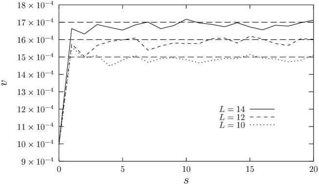
FIG. 1.: The spreading velocity $v$ vs. sparseness $s$ for three values of the genotype length $L$; $\mu_{\ell}=10^{-4}$, $\mu_{s}=10^{-3}$, flat fitness landscape. The dashed lines indicate the mean field value $v=\mu_{s}+L\mu_{\ell}/2$.

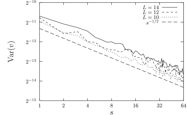
FIG. 2.: The fluctuations $\text{Var}(v)$ of the spreading velocity $v$ vs. sparseness $s$ for for three values of the genotype length $L$; $\mu_{\ell}=10^{-4}$, $\mu_{s}=10^{-3}$, flat fitness landscape. The dashed line represent the law $\text{Var}(v)\sim s^{-1/2}$ .

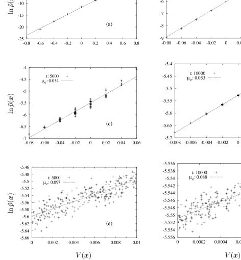
FIG. 3.: Numerical check for long-range mutations. In the simulations we set $L=8$, $\mu_{\ell}=0.1$ and $\mu_{s}=0$. We varied ${\mathcal{H}}$ (a,b), ${\mathcal{J}}$ (c,d) and ${\mathcal{K}}$ (e,f), setting all other parameters to zero. (a) ${\mathcal{H}}=0.01$, ${\mathcal{J}}=0$, ${\mathcal{K}}=0$; (b) ${\mathcal{H}}=0.001$, ${\mathcal{J}}=0$, ${\mathcal{K}}=0$; (c) ${\mathcal{H}}=0$, ${\mathcal{J}}=0.01$, ${\mathcal{K}}=0$; (d) ${\mathcal{H}}=0$, ${\mathcal{J}}=0.001$, ${\mathcal{K}}=0$; (e) ${\mathcal{H}}=0$, ${\mathcal{J}}=0$, ${\mathcal{K}}=0.1$; (f) ${\mathcal{H}}=0$, ${\mathcal{J}}=0$, ${\mathcal{K}}=0.01$. In the figures $t$ indicates the number of generations, $\mu_{e}$ the reciprocal of the slope of linear regression.

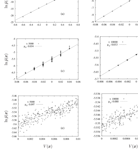
FIG. 4.: Numerical check for short-range mutations. In the simulations we set $L=8$, $\mu_{\ell}=0$ and $\mu_{s}=0.1$. We varied ${\mathcal{H}}$ (a,b), ${\mathcal{J}}$ (c,d) and ${\mathcal{K}}$ (e,f), setting all other parameters to zero. (a) ${\mathcal{H}}=0.1$, ${\mathcal{J}}=0$, ${\mathcal{K}}=0$; (b) ${\mathcal{H}}=0.01$, ${\mathcal{J}}=0$, ${\mathcal{K}}=0$; (c) ${\mathcal{H}}=0$, ${\mathcal{J}}=0.01$,${\mathcal{K}}=0$; (d) ${\mathcal{H}}=0$, ${\mathcal{J}}=0.001$, ${\mathcal{K}}=0$; (e) ${\mathcal{H}}=0$, ${\mathcal{J}}=0$, ${\mathcal{K}}=0.01$; (f) ${\mathcal{H}}=0$, ${\mathcal{J}}=0$, ${\mathcal{K}}=0.001$. In the figures $t$ indicates the number of generations, $\mu_{e}$ the reciprocal of the slope of linear regression.

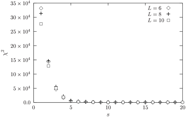
FIG. 5.: Scaling of the average square difference from linear regression, $\chi^{2}$ vs. sparseness $s$, for three values of the genotype length $L$; $\mu_{\ell}=0.1$, $\mu_{s}=0.1$, ${\mathcal{H}}=0$, ${\mathcal{J}}=0$, ${\mathcal{K}}=0.1$. Averages taken over 20 runs.

$V$	$L=6$			$L=8$			$L=10$			$L=12$
	$\mu_{e}^{(0)}$	$\overline{\mu}_{e}$	$s_{c}$	$\mu_{e}^{(0)}$	$\overline{\mu}_{e}$	$s_{c}$	$\mu_{e}^{(0)}$	$\overline{\mu}_{e}$	$s_{c}$	$\mu_{e}^{(0)}$	$\overline{\mu}_{e}$	$s_{c}$
${\mathcal{H}}$	0.035	0.045	3	0.025	0.035	3	0.020	0.030	2	0.017	0.027	2
${\mathcal{J}}$	0.071	0.082	4	0.053	0.063	4	0.042	0.052	4	0.035	0.045	3
${\mathcal{K}}$	0.080	0.105	6	0.090	0.105	6	0.096	0.107	6	0.098	0.111	3

TABLE I.: Effettive temperature $\mu_{e}$ for several values of the genotype length $L$ and parameters of the fitness $V(\boldsymbol{x})$, Eq (4). Here $\mu_{s}=0.1$, $\mu_{\ell}=0.01$; the row labeled ${\mathcal{H}}$ stands for ${\mathcal{H}}=0.1$, ${\mathcal{J}}={\mathcal{K}}=0$, the row labeled ${\mathcal{J}}$ stands for ${\mathcal{J}}=0.1$, ${\mathcal{H}}={\mathcal{K}}=0$, the row labeled ${\mathcal{K}}$ stands for ${\mathcal{K}}=0.1$, ${\mathcal{H}}={\mathcal{J}}=0$. We report the value or $\mu_{e}^{(0)}$ for sparseness $s=0$ (only small-range mutations) and the average value $\overline{\mu}_{e}$ for $s>s_{c}$, where $s_{c}$ is estimated visually from the plot of data (see also Fig. 5).

REFERENCES

- [1] R.A. Fisher, The genetical theory of natural selection (Dover, New York 1930).
- [2] S. Wright, The Roles of Mutation, Inbreeding, Crossbreeding, and Selection in Evolution, Proc. 6th Int. Cong. Genetics, Ithaca, 1, 356 (1932).
- [3] F. Bagnoli and M. Bezzi, Phys. Rev. Lett. 79, 3302 (1997), and cond-mat/9708101.
- [4] F. Bagnoli and M. Bezzi, Annual Review of Computational Physics VIII (2000)
- [5] F. Bagnoli and M. Bezzi, Path Integral Formulation of Evolving Ecosystems, in Path Integrals from peV to TeV, Edited by R. Casalbuoni et.al.(World Scientific, Singapore 1999) p. 493.
- [6] S. Gould and N. Elredge, Paleobiology 3, 114 (1997); Nature 366, 223 (1993).
- [7] E. Mayr, Populations, species and evolution (Harvard University Press, Cambridge Mass. 1970).
- [8] J. Maynard Smith, Evolutionary genetics (Oxford University Press, Oxford 1998).
- [9] D. J. Watts and S. H. Strogatz, Nature 393, 440 (1998).
- [10] R. Monasson, Eur. Phys. Jour. B 12, 60 (1999).
- [11] M. Kimura, The neutral theory of molecular evolution (Cambridge University Press, Cambridge 1983).
- [12] A. S. Kondrashov and F. A. Kondrashov, Nature 400, 351 (1999).
- [13] U. Dieckmann and M. Doebeli, Nature 400, 354 (1999).
- [14] W. Eigen, Naturwissenshaften 58, 465 (1971); W. Eigen and P. Schuster, Naturwissenshaften 64, 541 (1977).
- [15] M. Doebeli, J. Evol. Biol. 9, 893 (1999).
- [16] M. Doebeli, J. Evol. Biol. 9, 893 (1999); U. Dieckmann and M. Doebeli, Nature 400, 354 (1999).
- [17] F. Bagnoli and P. Lió, J. Theor. Biol. 173, 271 (1995).
- [18] D. L. Hartle, A Primer of Population Genetics, 2nd ed. (Sinauer, Sunderland, Massachusetts, 1988).
- [19] L. Peliti, Fitness Landscapes and Evolution, in Physics of Biomaterials: Fluctuations, Self-Assembly and Evolution, Edited by T. Riste and D. Sherrington (Kluwer, Dordrecht 1996) pp. 287-308, and cond-mat/9505003.
- [20] M. Argollo de Menezes, C.F. Moukarzel and T.J.P. Penna, Europhys. Lett. vol. 50, 5 (2000) and cond-mat/9903426.
- [21] I. Leuthäusser, J. Stat. Phys. 48, 343 (1987).
- [22] P. Tarazona, Phys. Rev. A 45, 6038 (1992).
- [23] T. Wiehe, E. Baake and P. Schuster, J. Theor. Biol. 177, 1 (1995).
- [24] http://www.docs.unifi.it/