A Quantum Analogue of the Jarzynski Equality

Understanding nonequilibrium quantum dynamics well be an important problem in the next century; new types of quantum devices, for instance, may function in their nonequilibrium states. In fact, it has been theoretically shown that quantum ratchet systems, which have the potential for being a new type of quantum device, function well in competitive situations between thermal relaxation and external driving, which are extremely nonequilibrium conditions.${}^{\hbox{\immediate{\bf{?}},\penalty 1000\hskip 0.91003pt plus 0.70004pt minus 0.70004pt{\bf{?}},\penalty 1000\hskip 0.91003pt plus 0.70004pt minus 0.70004pt{\bf{?}})}}$ A framework of theoretical methods for understanding such systems, however, is still under development. In this letter, we shall develop one equality which holds during a nonequilibrium process accompanied with thermal relaxation and external driving. This equality is a quantum analogue of the Jarzynski equality.${}^{\hbox{\immediate{\bf{?}},\penalty 1000\hskip 0.91003pt plus 0.70004pt minus 0.70004pt{\bf{?}})}}$ Considering such equality raises important issues regarding quantum nonequilibrium thermodynamics.

Consider the situation in which a classical system interacts with an isothermal heat bath characterized by an inverse temperature $\beta$. In this case, the system will become a thermal equilibrium state after a sufficiently long relaxation time. Next we assume that the system depends on a (macroscopic) parameter $\lambda$. If we change the parameter $\lambda$ infinitely slowly from $0$ to $1$, the system becomes another thermal equilibrium state corresponding to $\lambda=1$ from an equilibrium state with $\lambda=0$. When the operation is sufficiently slow (switching time $t_{s}$ is much larger), that is, when the system remains in quasistatic equilibrium during a switching process, the total work $W(t_{s}=\infty)$ performed on the system by the outside through the parameter $\lambda$ is identical to the Helmholtz free-energy difference $\Delta F$ between the initial state and the final one:

$$W(t_{s}=\infty)=\Delta F\equiv F_{0}-F_{1}\enspace,$$

where $F_{\lambda}$ is the Helmholtz free energy of the thermal equilibrium state with $\lambda$. If we operate the switching much faster, that is, a finite $t_{s}$, the work must be larger than the free-energy difference:

$$W(t_{s})\geq\Delta F\enspace.$$

This inequality represents the least-work principle. Extra work is required for a faster switching process because of thermodynamic stability. This extra work is released into the heat bath after the operation, when the system interacts with the isothermal heat bath.

In 1997, Jarzynski presented an equality which differs from the above inequality in the same situation.${}^{\hbox{\immediate{?},\penalty 1000\hskip 0.91003pt plus 0.70004pt minus 0.70004pt{?})}}$ His result is expressed by the following form:

$$\langle\exp(-\beta W(t_{s}))\rangle_{path}=\exp(-\beta\Delta F)\enspace.$$ (1)

This is called the Jarzynski equality. The brackets $\langle\dots\rangle_{path}$ mean taking the ensemble average along a single path during the switching process. An initial state is chosen from a thermal equilibrium ensemble with $\beta$ and $\lambda=0$. The dynamics of the system during the process can be taken as an arbitrary one that can express the thermal relaxation. If Monte Carlo dynamics, for instance, is used, one path corresponds to a single sampling series. Jarzynski also showed that the above equality holds in several dynamics such as Monte Carlo dynamics, Nosé-Hoover dynamics, Langevin dynamics, and even Hamiltonian dynamics without a thermal heat bath.${}^{\hbox{\immediate{?})}}$ This equality is general since it involves the least-work principle mentioned above.

In this letter, we consider an analogue of the Jarzynski equality in quantum situations. Let us define several notations and quantities. We denote the Hamiltonian of the system as ${\cal H}_{\lambda(t)}$, and $\lambda(t)$ a switching parameter operated by the outside at time $t$. A partition function $Z_{\lambda}$ and the Helmholtz free energy $F_{\lambda}$ are expressed as follows:

$$Z_{\lambda(t)} ={\rm Tr}\exp(-\beta{\cal H}_{\lambda(t)})\enspace,$$ (2)

$$F_{\lambda(t)} =-\beta^{-1}\ln Z_{\lambda(t)}(\beta)\enspace.$$ (3)

The work operator $\hat{W}(t)$ during a time interval $[0,t]$ is defined by the following:

$$\hat{W}(t)\equiv\int_{0}^{t}ds{{\displaystyle{\partial\lambda(s)}}\over{\displaystyle{\partial s}}}{{\displaystyle{\partial{\cal H}_{\lambda(s)}}}\over{\displaystyle{\partial\lambda}}}\enspace.$$ (4)

If $\lambda$ is not a macroscopic parameter, this definition does not correspond to the intuitive view of work. Here, we only consider the case where $\lambda$ is a macroscopic parameter. Using a density matrix of the system $\rho(t)$, we get the expression of the total average work $\langle\hat{W}(t)\rangle$ in the switching process as

$$\langle\hat{W}(t)\rangle\equiv{\rm Tr}\left\{\int_{0}^{t}ds{{\displaystyle{\partial\lambda(s)}}\over{\displaystyle{\partial s}}}{{\displaystyle{\partial{\cal H}_{\lambda(s)}}}\over{\displaystyle{\partial\lambda}}}\rho(s)\right\}\enspace.$$ (5)

In the present situation, the least-work principle also holds

$$\langle\hat{W}(t)\rangle\geq\Delta F\enspace$$

for arbitrary switching processes. The equal sign is valid for quasistatic limits as well as the classical case.

Let us consider a path average of exponentiated work corresponding to the left-hand side of the classical Jarzynski equality. In the present situation, taking the path average is difficult because we do not know how an ensemble reproduces thermal relaxation in the quantum dynamics. Therefore, we use the density matrix approach here. Then, the classical path average can be directly interpreted into the quantum situation:

$$\langle\exp\left(-\beta W(t)\right)\rangle_{path}\approx\overline{\exp\left(-\beta\hat{W}(t)\right)}\equiv{\rm Tr}\left\{\lim_{N\to\infty}{\cal T}\prod_{n=0}^{N-1}\left\{\widetilde{{\cal P}}_{\lambda(t_{n+1})}^{\delta t}e^{-\beta{\cal H}_{\lambda(t_{n+1})}}e^{+\beta{\cal H}_{\lambda(t_{n})}}\right\}\frac{e^{-\beta{\cal H}_{\lambda(0)}}}{Z_{\lambda(0)}}\right\}\enspace,$$ (6)

where $\delta t=t/N$ and $t_{n}=n\delta t$. The term $e^{-\beta{\cal H}_{\lambda(t_{n+1})}}e^{+\beta{\cal H}_{\lambda(t_{n})}}$ corresponds to exponentiated infinitesimal work. In this expression, $\widetilde{{\cal P}}_{\lambda(t)}^{\delta t}$ is an infinitesimal time-evolution superoperator for a tiny step $\delta t$ at time $t$ defined by

$$\widetilde{{\cal P}}_{\lambda(t)}^{\delta t}=e^{{\cal L}(t)\delta t}\enspace,$$

where ${\cal L}(t)$ is the Liouville superoperator governing the time evolution of the density matrix:

$$\frac{\partial\rho(t)}{\partial t}={\cal L}(t)\rho(t)\enspace.$$

Details of the dynamics are not important at this time. Its least property is determined in the following. ${\cal T}$ shows that the time ordering is taken as an increase in the left direction.

This is actually the analogue of the classical path average. It can be expressed as follows:

$$\langle\exp(-\beta W(t))\rangle_{path}=\lim_{N\to\infty}\int dx_{N}\prod_{n=0}^{N-1}\left\{\int dx_{n}{\cal P}_{\lambda(t_{n+1})}^{\delta t}(x_{n+1}|x_{n})e^{-\beta\delta w(x_{n})}\right\}\frac{e^{-\beta{\cal H}_{\lambda(t_{0})}(x_{0})}}{Z_{\lambda(0)}}\enspace,$$ (7)

where $x_{n}$ denotes canonical variables describing the classical system and an infinitesimal work, $\delta w(x_{n})$ is defined by ${\cal H}_{\lambda(t_{n+1})}(x_{n})-{\cal H}_{\lambda(t_{n})}(x_{n})$. ${\cal P}_{\lambda(t_{n+1})}^{\delta t}(x_{n+1}|x_{n})$ is an infinitesimal time-evolution operator such as a transition probability for the Monte Carlo dynamics. From this form we can understand that eq. (6) is a straight extension of classical situations.

In this way, we obtain the quantum analogue of the path-averaged exponentiated work. In the next step, we must show that the above expression is identical to the exponentiated Helmholtz free-energy difference. For this purpose, we use the fundamental property of the Liouville superoperator: it is vanished by the one density matrix that is the thermal equilibrium distribution $\propto\exp\left(-\beta{\cal H}_{\lambda(t)}\right)$, because the system always interacts with the thermal heat bath in the present case. Such distribution, of course, depends on time $t$. That is, $\exp\left(-\beta{\cal H}_{\lambda(t)}\right)$ is a singular solution of the dynamics. In this sense, a part of the exponentiated infinitesimal work does not evolve:

$$\widetilde{{\cal P}}_{\lambda(t_{n+1})}^{\delta t}e^{-\beta{\cal H}_{\lambda(t_{n+1})}}=e^{-\beta{\cal H}_{\lambda(t_{n+1})}}\enspace.$$

Finally, we obtain

$${\rm Tr} \left\{\lim_{N\to\infty}{\cal T}\prod_{n=0}^{N-1}\left\{\widetilde{{\cal P}}_{\lambda(t_{n+1})}^{\delta t}e^{-\beta{\cal H}_{\lambda(t_{n+1})}}e^{+\beta{\cal H}_{\lambda(t_{n})}}\right\}\frac{e^{-\beta{\cal H}_{\lambda(0)}}}{Z_{\lambda(0)}}\right\}$$

$$= \frac{1}{Z_{\lambda(0)}}{\rm Tr}\left\{\lim_{N\to\infty}\widetilde{{\cal P}}_{\lambda(t_{N})}^{\delta t}e^{-\beta{\cal H}_{\lambda(t_{N})}}e^{+\beta{\cal H}_{\lambda(t_{N-1})}}\dots\widetilde{{\cal P}}_{\lambda(t_{1})}^{\delta t}e^{-\beta{\cal H}_{\lambda(t_{1})}}e^{+\beta{\cal H}_{\lambda(0)}}e^{-\beta{\cal H}_{\lambda(0)}}\right\}$$

$$= \frac{1}{Z_{\lambda(0)}}{\rm Tr}\left\{\lim_{N\to\infty}\widetilde{{\cal P}}_{\lambda(t_{N})}^{\delta t}e^{-\beta{\cal H}_{\lambda(t_{N})}}e^{+\beta{\cal H}_{\lambda(t_{N-1})}}\dots\widetilde{{\cal P}}_{\lambda(t_{2})}^{\delta t}e^{-\beta{\cal H}_{\lambda(t_{2})}}e^{+\beta{\cal H}_{\lambda(t_{1})}}e^{-\beta{\cal H}_{\lambda(t_{1})}}\right\}$$

$$\vdots$$

$$= \frac{1}{Z_{\lambda(0)}}{\rm Tr}\left\{e^{-\beta{\cal H}_{\lambda(t)}}\right\}\enspace.$$

Thus, the following equality

$$\overline{\exp\left(-\beta\hat{W}(t)\right)}=\frac{Z_{\lambda(t)}}{Z_{\lambda(0)}}$$

is proofed. This is the quantum analogue of the classical Jarzynski equality, the “quantum Jarzynski equality.”

It should be noted that this expression is valid in pure quantum dynamics as in classical dynamics. In pure dynamics, an operation of the superoperator on an arbitrary operator $A$, $\widetilde{{\cal P}}_{\lambda(t_{n+1})}^{\delta t}A$, is identical to $e^{-i{\cal H}_{\lambda(t_{n+1})}\delta t/\hbar}Ae^{i{\cal H}_{\lambda(t_{n+1})}\delta t/\hbar}$. Then, all the infinitesimal time-evolution superoperators are effectively identity operators. Finally, we obtain the exponentiated free-energy difference again.

The quantum Jarzynski equality is formulated by an operator form. Thus, all the variables during the process are operators in contrast to the classical one. This property creates some difficulties in the decomposition of the time variable. If we change the definition of the infinitesimal exponentiated work slightly, for example, to $e^{+\beta{\cal H}_{\lambda(t_{n})}}e^{-\beta{\cal H}_{\lambda(t_{n+1})}}$ or $e^{-\beta({\cal H}_{\lambda(t_{n+1})}-{\cal H}_{\lambda(t_{n})})}$, it causes errors at each time. Denoting the error of order $O(\delta t)$ as $A_{t_{n}}$, that is, the exponentiated work is taken as $e^{-\beta{\cal H}_{\lambda(t_{n+1})}}e^{+\beta{\cal H}_{\lambda(t_{n})}}+A_{t_{n}}+O((\delta t)^{2})$, we obtain the final error as

$${{\displaystyle{1}}\over{\displaystyle{Z_{\lambda(0)}}}}{\rm Tr}\left[\lim_{N\to\infty}\left\{\sum_{l=0}^{N-1}\left({\cal T}{\prod_{n=l+1}^{N-1}}^{*}\widetilde{{\cal P}}_{\lambda(t_{n+1})}^{\delta t}e^{-\beta{\cal H}_{\lambda(t_{n+1})}}e^{+\beta{\cal H}_{\lambda(t_{n})}}\right)\widetilde{{\cal P}}_{\lambda(t_{l+1})}^{\delta t}A_{t_{l}}e^{-\beta{\cal H}_{\lambda(t_{l})}}+O((\delta t)^{2})\right\}\right]\enspace,$$ (8)

where ${\prod_{n=l+1}^{N-1}}^{*}$ represents the omission of the term $\prod_{n=N}^{N-1}$. At the limit $N\to\infty$ this error may remain, since $N$ terms of the order $O(\delta t)=O(1/N)$ are collected. The higher-order errors may vanish because their number is $O(N)$ at most. Therefore, the small mistaken choice of the exponentiated infinitesimal work causes a serious error in the final result. In a practical situation, however, $A_{t_{n}}$ may be of the order $O(\delta t\times(t_{s})^{-1})$. For sufficiently large $t_{s}$, the final error is not serious.

To confirm the quantum Jarzynski equality, we numerically investigate a simple quantum system. We choose the spin $1/2$ system interacting with an isothermal heat bath and time-dependent magnetic field. Here, we consider a process in which the magnetic field is linearly reversed in a finite time interval. The Hamiltonian ${\cal H}_{s}(t)$ and the magnetic field $\lambda(t)$ at time $t$ are as follows:

$${\cal H}_{s}(t) =-\frac{\lambda(t)}{2}\sigma^{z}-\frac{1}{2}\Delta\sigma^{x}\enspace,$$

$$\lambda(t) =\lambda_{0}\left(1-2\frac{t}{t_{s}}\right)\enspace,$$

where $\sigma^{x}$ and $\sigma^{z}$ are Pauli matrices. The parameters $\Delta$ and $\lambda_{0}$ are constants taken as $\Delta=0.1$ and $\lambda_{0}=1$, respectively. Interaction between the system and the heat bath is described by $\gamma\sigma^{x}\sum_{\alpha}(a^{\dagger}_{\alpha}+a_{\alpha})$ ($\gamma$ is a coupling constant) and the bath is expressed by a set of harmonic oscillators $\sum_{\alpha}\hbar\omega_{\alpha}\left(a^{\dagger}_{\alpha}a_{\alpha}+1/2\right)$ , where $a^{\dagger}_{\alpha}(a_{\alpha})$ is a creation (annihilation) operator with a mode $\alpha$. $t_{s}$ is a switching interval. The dynamics starts at time $t=0$ with a thermal equilibrium state and finishes at time $t=t_{s}$. Using the projection technique${}^{\hbox{\immediate{\bf{?}})}}$ with the assumption that the heat bath is always in a thermal equilibrium state with an inverse temperature $\beta$, we obtain the equation of motion of the density matrix of the spin system $\rho(t)$ as

$$\frac{\partial\rho}{\partial t}=-\frac{i}{\hbar}\left[{\cal H}_{s}(t),\rho(t)\right]+\frac{\gamma^{2}}{\hbar^{2}}\Gamma(\rho)\enspace,$$ (9)

where $\Gamma$ is a relaxation term guaranteeing that the system will relax into an instantaneous thermal equilibrium state $\propto\exp(-\beta{\cal H}_{s}(t))$. If the Hamiltonian does not depend on time, this equation can express the thermal relaxation to a thermal equilibrium state. The explicit form of $\Gamma$ is so complicated that is not presented here, but can be essentially described by $\sigma^{x}$ (interaction between the spin and the bath) and the autocorrelation function of the thermal heat bath variables. For actual calculations we use the second-order perturbation for the coupling constant $\gamma$.

Figure 1 shows the results of numerical calculations. Several time series of the expectation value of work defined by eq. (5) are presented. Each time series has a different switching time $t_{s}$. The exact Helmholtz free-energy difference at the corresponding time and the result of the quantum Jarzynski equality are also shown. As switching time increases, the value of work is more converged into the exact Helmholtz free-energy difference, because the dynamics becomes closer to a quasistatic one. On the other hand, when $t_{s}$ is short, a nonadiabatic transition dominates the dynamics. Thus, the extra work is needed. The result of the quantum Jarzynski equality completely agrees with the exact Helmholtz free-energy difference.

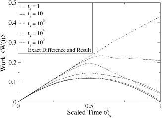
Fig.  1: Time series of the expectation value of work, the exact Helmholtz free-energy difference and the result of the quantum Jarzynski equality. Horizontal axis is taken to be scaled time $t/t_{s}$.

To summarize, we have constructed a quantum analogue of the Jarzynski equality. This equality connects a type of average of the exponentiated work operator during the switching process with the exact Helmholtz free-energy difference between an initial thermal equilibrium state and the final thermal equilibrium state, even though the actual final state of the process is not thermal equilibrium. We have also confirmed that the present equality works in practical calculations. In the spin 1/2 system with varying magnetic field interacting with the thermal heat bath, the result coincides with the exact difference of the Helmholtz free energy.

The present quantum Jarzynski equality includes the classical quality. In the classical limit, the density operator becomes a diagonal matrix, that is, the distribution function of the corresponding classical system. In this limit, the infinitesimal time-evolution operator describes only the transition between diagonal elements such as one of a Fokker-Planck operator. Then, the average part of the quantum one is similar to eq. (7).

It should be noted that the dynamics during the switching process can be chosen arbitrarily as one which has only the property that the time-dependent thermal equilibrium state $\propto\exp(-\beta{\cal H}_{\lambda(t)})$ is a singular solution of the dynamics. This property does not restrict the dynamics to Liouvillian dynamics with the projection technique such as eq. (9). Even though the singular solution $\exp(-\beta{\cal H}_{\lambda(t)})$ is unstable, the dynamics having such a singular solution can produce the same results. In this situation, however, other results derived from the dynamics are not physical.

It is known that the classical Jarzynski equality is related to the fluctuation theorem,${}^{\hbox{\immediate{\bf{?}},\penalty 1000\hskip 0.91003pt plus 0.70004pt minus 0.70004pt{\bf{?}},\penalty 1000\hskip 0.91003pt plus 0.70004pt minus 0.70004pt{\bf{?}})}}$ which is the relation of a distribution function of the entropy production rate, and is also valid in dynamics between nonequilibrium steady states.${}^{\hbox{\immediate{\bf{?}})}}$ Based on these findings, we can put forth several questions. What is a quantum analogue of the classical fluctuation theorem and how is the quantum Jarzynski equality extended into nonequilibrium steady dynamics? These problems are now in progress.

The author is grateful to N. Ito, S. Miyashita, and K. Saito for valuable discussions. This work was partly supported by Grants-in-Aid from the Ministry of Education, Science, Sports and Culture (No. 11740222).

References

- [1] S. Yukawa, M. Kikuchi, G. Tatara and H. Matsukawa; J. Phys. Soc. Jpn. 66, (1997), 2953.
- [2] P. Reimann, M. Grifoni and P. Hänggi; Phys. Rev. Lett. 79, (1997), 10.
- [3] G. Tatara, M. Kikuchi, S. Yukawa and H. Matsukawa; J. Phys. Soc. Jpn. 67, (1998), 1090.
- [4] C. Jarzynski; Phys. Rev. Lett. 78, (1997), 2690.
- [5] C. Jarzynski; Phys. Rev. E 56, (1997), 5018.
- [6] For example, R. Kubo, M. Toda and N. Hashitsume; Statistical Physics II, Nonequilibrium Statistical Mechanics, (Springer-Verlag, New York, 1991).
- [7] G. E. Crooks; Phys. Rev. E 60, (1999), 2721.
- [8] G. Gallavotti and E. G. D. Cohen; Phys. Rev. Lett. 74, (1995), 2694.
- [9] G. Gallavotti and E. G. D. Cohen; J. Stat. Phys. 80, (1995), 931.
- [10] T. Hatano; Phys. Rev. E 60, (1999), R5017.