Ohta-Jasnow-Kawasaki Approximation for Nonconserved Coarsening under Shear

Abstract

We analytically study coarsening dynamics in a system with nonconserved scalar order parameter, when a uniform time-independent shear flow is present. We use an anisotropic version of the Ohta-Jasnow-Kawasaki approximation to calculate the growth exponents in two and three dimensions: for $d=3$ the exponents we find are the same as expected on the basis of simple scaling arguments, that is $3/2$ in the flow direction and $1/2$ in all the other directions, while for $d=2$ we find an unusual behavior, in that the domains experience an unlimited narrowing for very large times and a nontrivial dynamical scaling appears. In addition, we consider the case where an oscillatory shear is applied to a two-dimensional system, finding in this case a standard $t^{1/2}$ growth, modulated by periodic oscillations. We support our two-dimensional results by means of numerical simulations and we propose to test our predictions by experiments on twisted nematic liquid crystals.

I Introduction

When a statistical system in its homogeneous disordered phase is suddenly quenched below the critical temperature, deep into a multi-phase coexistence region, a dynamical process known as coarsening, or phase-ordering, results: domains of the different ordered phases are formed and compete with each other in the attempt to break the symmetry and project the system on to one single equilibrium state [1]. An equivalent phenomenon occurs in the case of binary fluids: a system at the critical concentration tries to phase-separate after the quench, by forming domains of the two different components (spinodal decomposition). An interesting problem is the analysis of the dynamical evolution of these domains, and in particular the determination of their growth rate. In this aim a property shared by many statistical systems, called dynamical scaling, stating that space and time scale homogeneously in the equal-time two-point correlation function, $C(r,t)=f[r/L(t)]$, proves very useful. It is then natural to identify the length scale $L(t)$ as the typical size of the domains during coarsening. This length scale has generally a power-law dependence on time, $L(t)\sim t^{1/z}$, sometimes with logarithmic corrections. The determination of the exponent $z$ for many different statistical systems has been the object of much effort in the past years and we can say that ordinary coarsening is now quite well understood [1].

A related topic, which is attracting growing attention in recent years, is the problem of phase-ordering when the system is subject to an external shear. Apart from the great technological relevance of such a problem, especially in the case of spinodal decomposition, the basic theoretical understanding of the phenomena involved is far from being well established [2, 3, 4]. When a shear is present, domain growth is heavily affected by the presence of the induced flow and the dynamical scaling behavior is drastically different from the case of ordinary coarsening. In particular, two main points are worthy of careful investigation: First, the growth of the domains is anisotropic and therefore the dynamical evolution is described by more than one exponent. The determination of the shear exponents is, of course, of the uppermost importance. Secondly, it is not clear whether the shear causes an interruption of coarsening, the dynamical balance between growth and deformation giving rise to a stationary state (as argued in [5]), or, on the contrary, whether domain growth continues indefinitely. Experimental, numerical and theoretical evidence concerning both these points is still very tentative [6].

In the present work we perform a theoretical investigation of the coarsening dynamics in a statistical system with nonconserved scalar order parameter (model A, in the classification of Hohenberg and Halperin [7]), when a shear flow uniform in space is present. If, on one hand, such a model is unsuitable for describing spinodal decomposition in binary fluids, on the other hand it allows us to compute the growth exponents in any spatial dimension, in the context of a suitably modified version of the classic Ohta-Jasnow-Kawasaki (OJK) approximation [8]. When considering the relevance of nonconserved dynamics for an advance in our understanding of domain growth in the presence of a shear, we must take into account the fact that the only existing analytic calculations of the growth exponents for spinodal decomposition (conserved dynamics, or model B) have been performed in the limit of infinite dimension $N$ of the order parameter [9], where no saturation of coarsening is found. However, in that case the very concept of domains is meaningless and thus a calculation which takes into account the more physical case of a scalar order parameter is desirable. Besides, an understanding of the effect of shear on nonconserved coarsening is by itself an interesting problem, both from the theoretical and experimental point of view. Indeed, experiments have been performed in the past on twisted nematic liquid crystals [10], showing that these systems are a perfect test for analytical results in statistical models with nonconserved order parameter. Many results, from growth laws to persistence exponents, have been successfully tested on twisted nematic liquid crystals [11] and we therefore propose a shear experiment on such systems to check the results of our calculation.

We investigate two very different cases: in the first, a shear uniform in time is applied and the behavior of the system is analyzed asymptotically for very large times. In the second case, we consider a shear flow which is periodically oscillating in time and we study the properties of the model for times much longer than the period of the oscillation. The primary effect of the shear flow is naturally to stretch the domains in the direction of the flow, such that they can be roughly represented as highly elongated ellipsoids, with the growth taking place along the main axes. Two natural length scales therefore arise, $L_{\|}$ and $L_{\bot}$, the size of the domain along the largest and the smallest axes, respectively. The determination of the growth laws for these two length scales is the main objective of this work.

In the case of a time-independent shear, our results are nontrivial and, especially in two dimensions, quite unexpected. For $d=2$ our calculation gives $L_{\|}\sim\gamma^{1/2}t\,(\ln t)^{1/4}$ and $L_{\bot}\sim\gamma^{-1/2}\,(\ln t)^{-1/4}$, where $\gamma$ is the shear rate, while for $d=3$ we find $L_{\|}\sim\gamma t^{3/2}$ and $L_{\bot}\sim t^{1/2}$. The three-dimensional exponents are the same as one would expect on the basis of simple scaling arguments and are compatible with calculations for conserved dynamics in the large-$N$ limit [9]: the growth along the flow is enhanced by a factor $\gamma t$, while the transverse growth is unaffected by the shear. On the other hand, the two-dimensional result comes as quite a surprise: the short size of the domains $L_{\bot}$ goes asymptotically to zero for very large times, while the scale area grows as in the unsheared case, $L_{\|}L_{\bot}\sim t$. As we shall show, there are topological arguments supporting this last result. As long as our approach is valid, we do not find any evidence of the onset of a stationary state giving rise to an interruption of the coarsening process. However, in two dimensions our calculation breaks down when the thickness of the domains becomes comparable with the interfacial width. We cannot say what happens when this stage is reached, but it is possible that some kind of stationary state occurs in this regime. In the case of an oscillatory shear flow in two dimensions, we find $L_{\|}\sim t^{1/2}\,\sqrt{\gamma/\omega}\,f_{\parallel}(t)$ and $L_{\bot}\sim t^{1/2}\,\sqrt{\omega/\gamma}\,f_{\perp}(t)$, where $\omega$ is the frequency of the periodic flow: both length scales grow like $t^{1/2}$, but are modulated by oscillatory functions, $f_{\parallel}(t)$ and $f_{\perp}(t)$, with the same period as the flow and with mutually opposite phase. In this case also, therefore, we do not find any stationary state.

The structure of the paper is the following. In Section II we introduce the OJK approximation, with the appropriate modifications due to the presence of the shear. We end Section II by formulating some self-consistency equations for the matrix encoding the anisotropy of the domains (the elongation matrix). Given the technical difficulty of such equations, in Section III we present some simple geometric arguments useful to achieve a better understanding of the asymptotic behavior of the many quantities involved in the calculation. The explicit solution of the equations in two dimensions, together with the calculation of the growth exponents, is carried out in Section IV for a time independent shear rate and in Section V for an oscillatory shear rate, while in Section VI we solve the time-independent problem in three dimensions. In Section VII we present some numerical simulations in two dimensions, supporting our results, and in Section VIII we discuss a possible experimental test in the context of twisted nematic liquid crystals. Finally, we draw our conclusions in Section IX. A shorter account of part of this work can be found in [12].

II The OJK approach

The time evolution of a statistical system with nonconserved scalar order parameter $\phi(\vec{x},t)$ is described by the time-dependent Ginzburg-Landau equation [13]

$$\frac{\partial\phi(\vec{x},t)}{\partial t}=\nabla^{2}\phi(\vec{x},t)-V^{\prime}(\phi)\ ,$$ (1)

where $V(\phi)$ is a double-well potential. Under the hypothesis that the thickness $\xi$ of the interface separating different domains is much smaller than the size $L$ of the domains, it is possible to write an equation for the motion of the interface itself, assumed to be well localized in space. This is the Allen-Cahn equation [14], asserting that the velocity $v$ of the interface is proportional to the local curvature

$$v(\vec{x},t)=-{\vec{\nabla}\cdot\vec{n}(\vec{x},t)}\ ,$$ (2)

where $\vec{n}(\vec{x},t)$ is the unit vector normal to the interface and $\vec{\nabla}\cdot\vec{n}(\vec{x},t)$ is the curvature. The normal vector can be written in general as

$${\vec{n}(\vec{x},t)}=\frac{\vec{\nabla}m(\vec{x},t)}{|\vec{\nabla}m(\vec{x},t)|}\ ,$$ (3)

where $m(\vec{x},t)$ can be any field which is zero at the interface of the domain, defined by the vanishing of the order parameter $\phi(\vec{x},t)$. Given that this is the only restriction on the field $m(\vec{x},t)$, it is convenient not to use the order parameter itself in order to describe the motion of the interface via equation (2), but a smoother field [8]. Indeed, as we shall see, the principal effect of the OJK approximation is to produce a Gaussian distribution for the field $m(\vec{x},t)$, which would be particularly unsuitable for the highly non-Gaussian, double-peaked distribution of the order parameter $\phi(\vec{x},t)$.

From equations (2) and (3) we have

$$v(\vec{x},t)=-\sum_{a=1}^{d}\frac{\partial}{\partial x_{a}}\left(\frac{\partial_{a}m(\vec{x},t)}{|\vec{\nabla}m(\vec{x},t)|}\right)=-\frac{\nabla^{2}m(\vec{x},t)}{|\vec{\nabla}m(\vec{x},t)|}+\sum_{a,b=1}^{d}\frac{\partial_{a}m(\vec{x},t)\partial_{b}m(\vec{x},t)}{|\vec{\nabla}m(\vec{x},t)|^{2}}\ \frac{\partial_{a}\partial_{b}m(\vec{x},t)}{|\vec{\nabla}m(\vec{x},t)|}\ .$$ (4)

By considering a frame co-moving with the interface, we can write

$$0=\frac{dm(\vec{x},t)}{dt}=\frac{\partial m(\vec{x},t)}{\partial t}+\vec{v}_{tot}\cdot\vec{\nabla}m(\vec{x},t)\ .$$ (5)

If a shear flow is present, it can be taken into account by including in the total velocity $\vec{v}_{tot}$ of the interface, a contribution due to velocity field $\vec{u}$ induced by the shear

$${\vec{v}_{tot}}=v{\vec{n}}+{\vec{u}}\ ,$$ (6)

where $v{\vec{n}}$ is the curvature driven velocity, with direction orthogonal to the interface and modulus given by (4). By substituting relation (4) into equation (5) and by noting that $\vec{n}\cdot\vec{\nabla}m=|\vec{\nabla}m|$, we finally get the OJK equation

$$\frac{\partial m(\vec{x},t)}{\partial t}+\sum_{a=1}^{d}u_{a}\frac{\partial m(\vec{x},t)}{\partial x_{a}}=\nabla^{2}m(\vec{x},t)-\sum_{a,b=1}^{d}n_{a}(\vec{x},t)\;n_{b}(\vec{x},t)\frac{\partial^{2}m(\vec{x},t)}{\partial x_{a}\partial x_{b}}\ .$$ (7)

This is an exact relation for the field $m(\vec{x},t)$. The OJK equation is highly nonlinear due to the dependence of the vector $\vec{n}$ on the field $m$ through eq.(3). The OJK approximation [8] consists in replacing the factor $n_{a}n_{b}$ by its spatial average

$$D_{ab}(t)\equiv\langle n_{a}(\vec{x},t)n_{b}(\vec{x},t)\rangle\ .$$ (8)

Note that the elongation matrix $D_{ab}$ must satisfy the obvious sum rule

$$\sum_{a=1}^{d}D_{aa}(t)=1\ .$$ (9)

In the isotropic case (${\vec{u}}=0$) the elongation matrix is just $D_{ab}=\delta_{ab}/d$ by symmetry, and the OJK equation reduces to a simple diffusion equation with diffusion constant equal to $(d-1)/d$. On the other hand, when a shear flow is present the matrix $D_{ab}$ must encode the anisotropy induced by the shear and it must therefore depend on time, as the average shape of the domains does. The system of equations we have to solve is therefore

$$\frac{\partial m(\vec{x},t)}{\partial t}+\sum_{a=1}^{d}u_{a}\frac{\partial m(\vec{x},t)}{\partial x_{a}} = \nabla^{2}m(\vec{x},t)-\sum_{a,b=1}^{d}D_{ab}(t)\frac{\partial^{2}m(\vec{x},t)}{\partial x_{a}\partial x_{b}}\ ,$$ (10)

$$D_{ab}(t) = \left\langle\frac{\partial_{a}m(\vec{x},t)\;\partial_{b}m(\vec{x},t)}{\sum_{c}[\partial_{c}m(\vec{x},t)]^{2}}\right\rangle\ .$$ (11)

In this paper we will consider a space-uniform shear in the $y$ direction, with flow in the $x$ direction. The velocity profile is therefore given by

$${\vec{u}}=\gamma y{\vec{e}}_{x}\ ,$$ (12)

where $\gamma$ is the shear rate and ${\vec{e}}_{x}$ is the unit vector in the flow direction. In the present Section we will consider the case of a time-independent shear rate $\gamma$. A straightforward generalization of the calculation to the periodic case will be given in Section V.

By going into Fourier space we can rewrite equation (10) as

$$\frac{\partial m(\vec{k},t)}{\partial t}-\gamma k_{x}\frac{\partial m(\vec{k},t)}{\partial k_{y}}=\left(-\sum_{a=1}^{d}k_{a}^{2}+\sum_{a,b=1}^{d}D_{ab}(t)k_{a}k_{b}\right)m(\vec{k},t)\ .$$ (13)

Note that a naive scaling analysis of the left-hand side of this equation would give

$$L_{x}(t)\sim\gamma t\;L_{y}(t)\ ,$$ (14)

where $L_{x}$ and $L_{y}$ are the characteristic domain sizes in the $x$ and $y$ directions respectively. If we assume that the domain growth in the directions transverse to the flow is not modified by the shear, we obtain from (14) the results

$$L_{x}(t) \sim \gamma t^{3/2}$$ (15)

$$L_{y}(t) \sim t^{1/2}\ ,$$ (16)

where $L_{y}$ now represents any transverse direction. This is the simple scaling we mentioned in the Introduction. As we shall see, result (15) only holds in three dimensions, while a completely different situation occurs for $d=2$.

In order to solve equation (13) we perform the change of variables

$$q_{x} = k_{x}$$ (17)

$$q_{y} = k_{y}+\gamma k_{x}t$$ (18)

$$q_{a} = k_{a}\ \ ,\ \ \forall\ a\geq 3$$ (19)

$$\tau = t\ ,$$ (20)

introducing the field $\mu(\vec{q},\tau)\equiv m(\vec{k},t)$. The corresponding equation for $\mu$ reads

$$\frac{\partial\ln\mu(\vec{q},\tau)}{\partial\tau} = -q_{x}^{2}-(q_{y}-\gamma q_{x}\tau)^{2}-\sum_{a=3}^{d}q_{a}^{2}+$$ (21)

$$D_{11}(\tau)q_{x}^{2}+2D_{12}(\tau)q_{x}(q_{y}-\gamma q_{x}\tau)+D_{22}(\tau)(q_{y}-\gamma q_{x}\tau)^{2}+\sum_{a,b=3}^{d}D_{ab}(\tau)q_{a}q_{b}\ .$$ (22)

The original OJK equation (7), with a shear flow given by (12), is invariant under any transformation which preserves the sign of the product $xy$. In order to keep this symmetry, it is necessary for the elongation matrix $D_{ab}$ to have the following block-diagonal form

$$D_{1a}(t)=D_{2a}(t)=0\ \ \ ,\ \ \ D_{ab}(t)=D_{33}(t)\;\delta_{ab}\ \ \ ,\ \ \ \forall\ a,b\geq 3\ ,$$ (23)

where, to simplify the notation, we have used $D_{33}(t)$ to denote all the diagonal elements for $a\geq 3$. Equation (21) can now be integrated to give

$$\mu(\vec{q},\tau)=\mu(\vec{q},0)\;\exp\left[-\frac{1}{4}\sum_{ab}q_{a}R_{ab}(\tau)\;q_{b}\right]\ ,$$ (24)

with

$$R_{11}(\tau) = 4\int_{0}^{\tau}d\tau^{\prime}\;\{[1-D_{11}(\tau^{\prime})]+2\gamma\tau^{\prime}D_{12}(\tau^{\prime})+\gamma^{2}\tau^{\prime 2}[1-D_{22}(\tau^{\prime})]\}$$ (25)

$$R_{12}(\tau) = 4\int_{0}^{\tau}d\tau^{\prime}\;\{-D_{12}(\tau^{\prime})-\gamma\tau^{\prime}[1-D_{22}(\tau^{\prime})]\}$$ (26)

$$R_{22}(\tau) = 4\int_{0}^{\tau}d\tau^{\prime}\;[1-D_{22}(\tau^{\prime})]$$ (27)

$$R_{1a}(\tau) = R_{2a}(\tau)=0\ \ ,\ \ \forall\ a\geq 3$$ (28)

$$R_{ab}(\tau) = 4\delta_{ab}\int_{0}^{\tau}d\tau^{\prime}\;[1-D_{33}(\tau^{\prime})]\equiv R_{33}(\tau)\;\delta_{ab}\ \ ,\ \ \forall\ a,b\geq 3\ .$$ (29)

We can now go back to the original field $m(\vec{k},t)$, via the relation

$$m(\vec{k},t)=\mu(k_{x},k_{y}+\gamma k_{x}t,k_{3},\dots,k_{d},t)\ ,$$ (30)

to obtain

$$m(\vec{k},t)=m(k_{x},k_{y}+\gamma k_{x}t,k_{3},\dots,k_{d},0)\ \exp\left[-\frac{1}{4}\sum_{ab}k_{a}M_{ab}(t)\;k_{b}\right]\ ,$$ (31)

with

$$M_{11}(t) = R_{11}(t)+2\gamma tR_{12}(t)+\gamma^{2}t^{2}R_{22}(t)$$ (32)

$$M_{12}(t) = R_{12}(t)+\gamma tR_{22}(t)$$ (33)

$$M_{22}(t) = R_{22}(t)$$ (34)

$$M_{1a}(t) = M_{2a}(t)=0\ \ ,\ \ \forall\ a\geq 3$$ (35)

$$M_{ab}(t) = R_{33}(t)\;\delta_{ab}\equiv M_{33}(t)\;\delta_{ab}\ \ ,\ \ \forall\ a,b\geq 3\ .$$ (36)

Relation (31) can be better understood in real space: due to the shear flow, the field $m$ at point $(x,y,\dots)$, at time $t$, is the propagation of the initial condition at point $(x-\gamma yt,y,\dots)$. Note that, if we assume a Gaussian distribution for $m(\vec{k},0)$ (disordered initial condition), the field maintains a Gaussian distribution at all the times, due to the linearity of equation (10). In order to get the correlation of $m(\vec{x},t)$ in real space we have to average over the initial conditions

$$\langle m(\vec{k},0)m(\vec{k}^{\prime},0)\rangle=\sqrt{\Delta}\ \delta(\vec{k}+\vec{k}^{\prime})\ .$$ (37)

The equal time pair-correlation function of $m$ is therefore

$$C_{m}(\vec{x},\vec{x}^{\prime};t)\equiv\langle m(\vec{x},t)m(\vec{x}^{\prime},t)\rangle=\sqrt{\frac{(2\pi)^{d/2}\Delta}{\det M(t)}}\ \exp\left[-\frac{1}{2}\sum_{ab}r_{a}[M^{-1}]_{ab}(t)\;r_{b}\right]\ ,$$ (38)

where $r_{a}=x_{a}-x_{a}^{\prime}$. All the information on the domain growth is contained in the correlation matrix $M_{ab}(t)$. Indeed, the eigenvectors of $M_{ab}(t)$ give the principal elongation axes of the domains and the square roots of its eigenvalues give the domain sizes along these axes.

The correlation matrix is connected to the elongation matrix by equations (27) and (34). In order to close the problem we have thus to write another set of equations, relating $M_{ab}(t)$ and $D_{ab}(t)$, by exploiting relation (11). If we introduce the field $\varphi_{a}(\vec{x},t)\equiv\partial_{a}m(\vec{x},t)$, we can write

$$D_{ab}(t)=\int{\cal D}P(\varphi)\;\frac{\varphi_{a}(\vec{x},t)\varphi_{b}(\vec{x},t)}{\sum_{c}\varphi_{c}(\vec{x},t)^{2}}=\frac{1}{2}\int_{0}^{\infty}dy\;\int{\cal D}P(\varphi)\;e^{-\frac{1}{2}y\sum_{c}\varphi_{c}(\vec{x},t)^{2}}\;\varphi_{a}(\vec{x},t)\varphi_{b}(\vec{x},t)\ ,$$ (39)

and we have thus to work out the probability distribution ${\cal D}P(\varphi)$. The field $\varphi$ is Gaussian and therefore we just need to compute its correlator. From equation (38) we have

$$\langle\varphi_{a}(\vec{x},t)\varphi_{b}(\vec{x},t)\rangle=\kappa\;[M^{-1}]_{ab}(t)\ \ \ \ \ ,\ \ \ \ \ \kappa=\sqrt{\frac{(2\pi)^{d/2}\Delta}{\det M(t)}}\ ,$$ (40)

and therefore

$${\cal D}P(\varphi)=\frac{1}{Z}\;\exp\left[-\frac{1}{2\kappa}\sum_{ab}\varphi_{a}(\vec{x},t)M_{ab}(t)\varphi_{b}(\vec{x},t)\right]\,{\cal D}\varphi\ ,$$ (41)

where the constant $Z$ normalizes the distribution. By defining

$$N_{ab}(y,t)=M_{ab}(t)+y\;\delta_{ab}\ ,$$ (42)

and by performing the rescaling $\varphi\to\varphi\sqrt{\kappa}$, $y\to y/\kappa$, we can write

$$D_{ab}(t) = \frac{1}{2}\int_{0}^{\infty}dy\;\frac{\int{\cal D}\varphi\;e^{-\frac{1}{2}\sum_{a^{\prime}b^{\prime}}\varphi_{a^{\prime}}(\vec{x},t)N_{a^{\prime}b^{\prime}}(y,t)\varphi_{b^{\prime}}(\vec{x},t)}\varphi_{a}(\vec{x},t)\varphi_{b}(\vec{x},t)}{\int{\cal D}\varphi\;e^{-\frac{1}{2}\sum_{a^{\prime}b^{\prime}}\varphi_{a^{\prime}}(\vec{x},t)M_{a^{\prime}b^{\prime}}(t)\varphi_{b^{\prime}}(\vec{x},t)}}$$ (43)

$$= \frac{1}{2}\sqrt{\det M(t)}\int_{0}^{\infty}dy\;\frac{[N^{-1}]_{ab}(y,t)}{\sqrt{\det N(y,t)}}\ .$$ (44)

Let us introduce the following parameters in order to explicitly write the relation above:

$$\sigma(t) \equiv M_{11}(t)M_{22}(t)-M_{12}(t)^{2}=R_{11}(t)R_{22}(t)-R_{12}(t)^{2}\ ,$$ (45)

$$\tau(t) \equiv M_{11}(t)+M_{22}(t)\ .$$ (46)

The first equation is a particular case of the more general relation $\det M=\det R$, a consequence of the fact that (19) is an orthogonal transformation. We can finally write

$$D_{11}^{22}(t) = \frac{1}{2}\sqrt{\sigma(t)M_{33}(t)^{d-2}}\int_{0}^{\infty}dy\;\frac{M_{22}^{11}(t)+y}{[y^{2}+\tau(t)y+\sigma(t)]^{\frac{3}{2}}[M_{33}(t)+y]^{\frac{d-2}{2}}}$$ (47)

$$-D_{12}(t) = \frac{1}{2}\sqrt{\sigma(t)M_{33}(t)^{d-2}}\int_{0}^{\infty}dy\;\frac{M_{12}(t)}{[y^{2}+\tau(t)y+\sigma(t)]^{\frac{3}{2}}[M_{33}(t)+y]^{\frac{d-2}{2}}}$$ (48)

$$D_{33}(t) = \frac{1}{2}\sqrt{\sigma(t)M_{33}(t)^{d-2}}\int_{0}^{\infty}dy\;\frac{1}{[y^{2}+\tau(t)y+\sigma(t)]^{\frac{1}{2}}[M_{33}(t)+y]^{\frac{d}{2}}}\ .$$ (49)

Relations (27), (34) and (48) form a closed set of equations for the correlation matrix $M_{ab}(t)$, or, equivalently, for the elongation matrix $D_{ab}(t)$. Before attempting to solve them, it is helpful to use physical considerations as a guide to the expected asymptotic form of the elongation matrix in the limit of very large times. To this aim, we will consider the case of a time-independent shear rate.

III Physical considerations on the elongation matrix

When a time-independent shear flow in the $x$ direction is present, the domains will be highly elongated along this direction and therefore most of the surface of the domains will tend to become parallel to the $x$ direction for very large times. We thus expect the following relation to hold

$$D_{11}(t)=\langle n_{x}n_{x}\rangle\to 0\ \ \ ,\ \ \ t\to\infty\ .$$ (50)

In the two-dimensional case, due to the sum rule (9), this relation implies

$$D_{22}(t)=\langle n_{y}n_{y}\rangle\to 1\ \ \ ,\ \ \ t\to\infty\ \ \ ,\ \ \ d=2\ ,$$ (51)

while in dimensions $d\geq 3$ it is not a priori clear whether both $D_{22}$ and $D_{33}$ remain nonzero or not. The only thing we can write is

$$D_{22}(t)+(d-2)D_{33}(t)\to 1\ \ \ ,\ \ \ t\to\infty\ \ \ ,\ \ \ d\geq 3\ .$$ (52)

With regard to the off-diagonal elements of the elongation matrix, it is not hard to convince oneself that the only nonzero ones can be $D_{12}(t)=D_{21}(t)=\langle n_{x}n_{y}\rangle$ (see equation (23)): indeed, due to the shear, the domains are elongated along two main axes which are not the $(xy)$ axes, unless $t=\infty$. Therefore, the sub-matrix $D_{ab}^{(xy)}(t)$ cannot be diagonal for any finite time. On the other hand, for $t\to\infty$ the two elongation axes become coincident with $(xy)$ and thus we expect that

$$D_{12}(t)\to 0\ \ \ ,\ \ \ t\to\infty\ .$$ (53)

It is finally clear that no qualitative difference can exist between $d=3$ and $d>3$. Indeed, in this paper we will explicitly state the results only for $d=2$ and $d=3$.

A useful exercise is to approximate a domain with an ellipsoid and compute the asymptotic value of $D_{ab}(t)$ as a function of the main axes. We will do this explicitly in two dimensions and we will just quote the main results for $d=3$. Let us call $L_{\|}$ and $L_{\bot}$ the largest and smallest axis of a two-dimensional ellipse. Besides, let $\theta$ be the tilt angle, that is the angle between the $x$ axis and the $L_{\|}$ axis (see Fig.1).

FIG. 1.: A two-dimensional domain in the elliptic approximation.

When a time-independent shear is applied, it is natural to assume for $t\to\infty$:

$$\theta\to 0\ \ \ ,\ \ \ L_{\|}\gg L_{\bot},$$ (54)

as an expression of the extreme elongation of the domain in the direction of the flow. We can now parametrise the tilted ellipse in the following way

$$x(\omega) = \frac{1}{2}L_{\|}\cos\omega-\frac{1}{2}\theta L_{\bot}\sin\omega$$ (55)

$$y(\omega) = \frac{1}{2}\theta L_{\|}\cos\omega+\frac{1}{2}L_{\bot}\sin\omega\ ,$$ (56)

with $\omega\in[0,2\pi]$ and where we have used the fact that $\theta$ is very small. The average of any quantity $A$ along the perimeter of the ellipse can now be calculated as,

$$\langle A\rangle=\frac{\int_{0}^{2\pi}d\omega\,\mu(\omega)A(\omega)}{\int_{0}^{2\pi}d\omega\,\mu(\omega)}\ ,$$ (57)

with the metric $\mu$ given by

$$\mu(\omega)=\frac{1}{2}(L_{\|}^{2}\sin^{2}\omega+L_{\bot}^{2}\cos^{2}\omega)^{1/2}\ .$$ (58)

It is useful to compute explicitly the normalizing factor in (57), i.e. the asymptotic perimeter of the ellipse,

$$\int_{0}^{2\pi}d\omega\,\mu(\omega)=\frac{1}{2}L_{\|}\;\int_{0}^{2\pi}d\omega\,(\sin^{2}\omega+\frac{L_{\bot}^{2}}{L_{\|}^{2}}\cos^{2}\omega)^{1/2}\sim 2L_{\|}+\frac{L_{\bot}^{2}}{L_{\|}}\ln\left(\frac{L_{\|}}{L_{\bot}}\right)\ ,$$ (59)

where we have used the relation $L_{\|}\gg L_{\bot}$. The asymptotic perimeter divided by the total area, $L_{\|}L_{\bot}$, is the interfacial density $\rho$ of the domains, which must be proportional to the energy density $E$ of the system. In the elliptic approximation we therefore have

$$E\sim\rho\sim\frac{2}{L_{\bot}}+\frac{L_{\bot}}{L_{\|}^{2}}\ln\left(\frac{L_{\|}}{L_{\bot}}\right)\ .$$ (60)

It will be interesting to compare this simple result with the one obtained from the OJK calculation in the next Section.

The vector normal to the interface can be easily found by imposing its orthogonality with the tangent vector $(\partial_{\omega}x,\partial_{\omega}y)$. This gives

$$n_{x}(\omega) = \frac{-\theta L_{\|}\sin\omega+L_{\bot}\cos\omega}{\mu(\omega)}$$ (61)

$$n_{y}(\omega) = \frac{L_{\|}\sin\omega+\theta L_{\bot}\cos\omega}{\mu(\omega)}\ .$$ (62)

We can now use the relations above to compute the elongation matrix of the ellipse, $D_{ab}=\langle n_{a}n_{b}\rangle$. By doing this we get

$$D_{11}(t) \sim \theta^{2}+\frac{L_{\bot}^{2}}{L_{\|}^{2}}\ln\left(\frac{L_{\|}}{L_{\bot}}\right)\to 0$$ (63)

$$D_{12}(t) \sim \;-\theta\to 0\ .$$ (64)

Note that a priori we cannot say which one of the two pieces of $D_{11}$ is going to dominate in the limit $t\to\infty$.

In dimension $d=3$ it is possible to perform a similar analysis, by introducing a third axis $L_{z}$ orthogonal to the $(xy)$ plane. The result is

$$D_{11}(t) \sim \theta^{2}+\frac{L_{\bot}^{2}}{L_{\|}^{2}}\to 0$$ (65)

$$D_{12}(t) \sim \;-\theta\to 0\ .$$ (66)

Besides, it is possible to show that if the ratio $L_{\bot}/L_{z}$ remains constant for $t\to\infty$, then both $D_{22}$ and $D_{33}$ are nonzero in this limit, and

$$D_{22}(t) = g_{2}(L_{\bot}/L_{z})$$ (67)

$$D_{33}(t) = g_{3}(L_{\bot}/L_{z})\ ,$$ (68)

where the two scaling functions must satisfy the relation

$$g_{2}(x)+g_{3}(x)=1\ .$$ (69)

The results of this Section confirm our expectation on the behavior of the elongation matrix and also give us some hint on the relation between the elongation matrix and the domain sizes, whose determination is, of course, our final goal.

IV Time independent shear in two dimensions

Finding a solution of the set of equations (27), (34) and (48) is, even in two dimensions and with a time-independent shear rate, not entirely straightforward. Therefore, we will first try to exploit a naive scaling analysis to find a suitable ansatz for the elongation matrix, and eventually we will modify our initial guess in such a way to self-consistently satisfy all our equations.

First, note that in two dimensions it is relatively simple to compute the integrals in (48). We obtain

$$D_{11}^{22}(t) = \frac{\tau(t)M_{22}^{11}(t)-2\sigma(t)-\sqrt{\sigma(t)}\;[2M_{22}^{11}(t)-\tau(t)]}{\tau(t)^{2}-4\sigma(t)}$$ (70)

$$D_{12}(t) = -M_{12}(t)\;\frac{\tau(t)-2\sqrt{\sigma(t)}}{\tau(t)^{2}-4\sigma(t)}\ ,$$ (71)

where it is easy to check that sum rule (9) is satisfied. Note that, of course, eqs.(70) are valid also for a time-dependent rate $\gamma(t)$ and we will therefore use them also in the next Section in the case of an oscillatory shear.

A crucial task is now to understand which terms dominate in the limit $t\to\infty$ in the equations above. A useful starting point is the correlation function in equation (38): if we assume that there are just two length scales, $L_{x}(t)$ and $L_{y}(t)$, a naive consequence we can draw is the following

$$M_{11}(t) \sim L_{x}(t)^{2}$$ (72)

$$M_{12}(t) \sim L_{x}(t)L_{y}(t)$$ (73)

$$M_{22}(t) \sim L_{y}(t)^{2}\ .$$ (74)

Moreover, the physics of the system suggests that

$$L_{x}(t)\gg L_{y}(t)\ .$$ (75)

Note that $L_{x}$ and $L_{y}$ do not in general coincide with $L_{\|}$ and $L_{\bot}$, as defined in the last Section. Indeed, this is the main difference between the naive approach and the final full solution in two dimensions. Relation (75) implies

$$M_{11}(t)\gg M_{12}(t)\gg M_{22}(t)\ ,$$ (76)

and thus

$$\tau(t)\sim M_{11}(t)\ \ \ \ ,\ \ \ \ \sigma(t)\ll M_{11}(t)^{2}\ .$$ (77)

In order to find the asymptotic behavior of equations (70) we need an extra relation. From definition (46), it seems natural to assume that $\sigma(t)\sim M_{11}(t)M_{22}(t)$, and therefore, from (76), that

$$\sigma(t)\gg M_{22}(t)^{2}\ .$$ (78)

What we are (naively) assuming is that there are no cancellations in $\sigma(t)$. This assumption will fail in the final solution, but it will only logarithmically fail, such that relation (78) will still be true. By using relations (77) and (78) in (70), we finally obtain

$$D_{11}(t) = \frac{\sqrt{\sigma(t)}}{M_{11}(t)}$$ (79)

$$D_{12}(t) = -\frac{M_{12}(t)}{M_{11}(t)}\ ,$$ (80)

at leading order for $t\to\infty$. Substituting relations (73) into (79) and (80), and by using the naive scaling relation $L_{x}(t)\sim\gamma tL_{y}(t)$, obtained in Section II, we get

$$D_{11}(t) = \frac{L_{y}(t)}{L_{x}(t)}\sim\frac{1}{\gamma t}$$ (81)

$$D_{12}(t) = -\frac{L_{y}(t)}{L_{x}(t)}\sim-\frac{1}{\gamma t}\ ,$$ (82)

where again we have assumed that $\sigma(t)\sim M_{11}(t)M_{22}(t)$. If we now use this asymptotic form of the elongation matrix in relations (27) and (34), we obtain

$$M_{11}(t) = \gamma^{2}t^{2}\;R_{22}(t)$$ (83)

$$M_{12}(t) = \gamma t\;R_{22}(t)$$ (84)

$$M_{22}(t) = R_{22}(t)\ ,$$ (85)

and

$$\sigma(t)=R_{11}(t)R_{22}(t)\ ,$$ (86)

with

$$R_{11}(t) = 4\gamma^{2}\int_{0}^{t}dt^{\prime}\;t^{\prime 2}D_{11}(t^{\prime})$$ (87)

$$R_{22}(t) = 4\int_{0}^{t}dt^{\prime}\;D_{11}(t^{\prime})\ ,$$ (88)

always at leading order. Relations (84) are consistent with equation (76), and by substituting (84) into (80) we find self-consistently the asymptotic form $D_{12}(t)\sim-1/\gamma t$. Moreover, by assuming once again that $\sigma(t)\sim M_{11}(t)M_{22}(t)$ and by substituting (84) into (79) we get $D_{11}(t)\sim 1/\gamma t$ and all our assumptions seem thus to be self-consistent. Unfortunately, this is not the case and it is not hard to understand that something is going wrong. Indeed, if we now plug into equation (79) the form of $\sigma(t)$ coming from equation (86), rather than the naive assumption $\sigma(t)\sim M_{11}(t)M_{22}(t)$, we get the following self-consistent equation for $D_{11}(t)$:

$$D_{11}(t)=\frac{\sqrt{R_{11}(t)R_{22}(t)}}{\gamma^{2}t^{2}\ R_{22}(t)}=\frac{1}{\gamma t^{2}}\left(\frac{\int_{0}^{t}dt^{\prime}\;t^{\prime 2}D_{11}(t^{\prime})}{\int_{0}^{t}dt^{\prime}\;D_{11}(t^{\prime})}\right)^{1/2}\ .$$ (89)

If we insert into the r.h.s. of this equation the asymptotic form of $D_{11}$ found above, we find an unpleasant surprise, that is

$$D_{11}(t)=\frac{a}{\gamma t\,\sqrt{\ln\gamma t}}\ ,$$ (90)

with $a=1/\sqrt{2}$, in contradiction with (81). However, the situation is far from being desperate, because if we try this very form of $D_{11}$ in equation (89) we fortunately find self-consistency with $a=1/2$. Our initial result (81) only failed to capture a logarithmic correction and it is possible to check that, with this new form of $D_{11}$, we recover all the relevant relations of this Section, namely (88), (86), (84), (80), (79), (78), (77) and (76), but not (81).

Summarizing, the correct final form of the elongation matrix in the two-dimensional case is therefore (always at leading order for $t\to\infty$):

$$D_{11}(t) = \frac{1}{2\gamma t\,\sqrt{\ln\gamma t}}$$ (91)

$$D_{12}(t) = -\frac{1}{\gamma t}$$ (92)

$$D_{22}(t) = 1-D_{11}(t)\ ,$$ (93)

while equation (81) is not correct. From (88) we have

$$R_{11}(t) = \frac{\gamma\;t^{2}}{\sqrt{\ln\gamma t}}$$ (94)

$$R_{22}(t) = \frac{4\sqrt{\ln\gamma t}}{\gamma}\ ,$$ (95)

whereas, from (84), the correlation matrix is

$$M_{11}(t) = 4\gamma t^{2}\,\sqrt{\ln\gamma t}$$ (96)

$$M_{12}(t) = 4t\,\sqrt{\ln\gamma t}$$ (97)

$$M_{22}(t) = \frac{4\sqrt{\ln\gamma t}}{\gamma}$$ (98)

$$\sigma(t) = 4t^{2}\ .$$ (99)

It is possible to see now that the critical assumption which went wrong in our initial analysis was $\sigma(t)\sim M_{11}(t)M_{22}(t)$. Indeed, from equations (97) we see that $\sigma(t)$ is smaller than this, because there are some non-trivial cancellations in the determinant of $M_{ab}$. For this same reason, one should not be misled by the fact that apparently in (97) the determinant of $M_{ab}$ is null: we did not write the sub-leading contributions to the correlation matrix which make $\sigma(t)\sim t^{2}\ll t^{2}\ln t$.

In order to obtain the domain size along the principal elongation axes, $L_{\|}(t)$ and $L_{\bot}(t)$, we have to find the eigenvalues $\lambda_{1}(t)$ and $\lambda_{2}(t)$ of $M_{ab}(t)$. This is easily done by recalling that the characteristic polynomial is just $\lambda^{2}-\tau\lambda+\sigma$, where $\tau$ and $\sigma$ are the trace and the determinant of $M_{ab}(t)$, respectively (cfr. eq.(46)). The final result for the two-dimensional case is:

$$L_{\|}(t) = \sqrt{\lambda_{1}(t)}=\sqrt{\tau(t)}=2\sqrt{\gamma}\;t\ (\ln\gamma t)^{1/4}$$ (100)

$$L_{\bot}(t) = \sqrt{\lambda_{2}(t)}=\sqrt{\frac{\sigma(t)}{\tau(t)}}=\frac{1}{\sqrt{\gamma}\;(\ln\gamma t)^{1/4}}\ .$$ (101)

Note how striking the effect of the shear is in two dimensions: the size of the domains along the minor axis shrinks to zero, even though very slowly, for $t\to\infty$. The asymptotic effect of this unlimited narrowing of the domains for very large times is still unclear to us. However, we do expect our approach to break down when $L_{\bot}(t)$ becomes of the same order as the interface thickness $\xi$, when equation (2) ceases to be valid. This happens after a very large time, of the order $\exp(1/\gamma^{2}\xi^{4})$. What we can say is that, if a steady state exists, it can be reached only when the thickness of the domains becomes comparable with the interface width.

An important feature of the solution we have found is the failure of standard $(x,y)$ scaling. In order to appreciate this fact, we have to remember that, even though $L_{\parallel}$ and $L_{\perp}$ are the natural domain sizes along the eigen-axes of the correlation matrix, other length scales can be defined, as shown in Fig.2:

FIG. 2.: The length scales $L_{x}$, $L_{y}$, $H_{x}$ and $H_{y}$.

First of all, we have $L_{x}$ and $L_{y}$: from the correlation function (38), it follows that

$$L_{x}(t) = \frac{1}{\sqrt{[M^{-1}]_{11}}}$$ (102)

$$L_{y}(t) = \frac{1}{\sqrt{[M^{-1}]_{22}}}\ ,$$ (103)

and from (97) we get

$$L_{x}(t) = \frac{\sqrt{\gamma}\,t}{(\ln\gamma t)^{1/4}}$$ (104)

$$L_{y}(t) = \frac{1}{\sqrt{\gamma}\,(\ln\gamma t)^{1/4}}\ .$$ (105)

Secondly, we can define $H_{x}$ and $H_{y}$, as the maximum extension of the domain in the $x$ and $y$ directions, that is

$$H_{x} = L_{\parallel}\cos\theta$$ (106)

$$H_{y} = L_{\parallel}\sin\theta\ ,$$ (107)

where $\theta$ is the usual tilt angle (see Fig.1), which can be easily computed from the eigenvectors of $M$. These are

$$\vec{e}_{\|}=\left(1,\frac{1}{\gamma t}\right)\ \ \ ,\ \ \ \vec{e}_{\bot}=\left(-\frac{1}{\gamma t},1\right)\ ,$$ (108)

and therefore

$$\theta=\frac{1}{\gamma t}\ .$$ (109)

In this way we have

$$H_{x}(t) = 2\sqrt{\gamma}t\,(\ln\gamma t)^{1/4}$$ (110)

$$H_{y}(t) = \frac{2(\ln\gamma t)^{1/4}}{\sqrt{\gamma}}\ .$$ (111)

In the absence of shear all these length scales would coincide, that is we would have $L_{\parallel}=L_{x}=H_{x}$ and $L_{\perp}=L_{y}=H_{y}$. With the shear this is no longer true, simply because $M_{12}\neq 0$. Still, we would expect these length scales to differ only by some constant factors, such that they would all be of the same order asymptotically in time. If this situation held, we would have a standard $(x,y)$ scaling, even though with anisotropic domains. However, in two dimensions the situation is very different, because the length scales above differ by logarithmic corrections. More precisely, we have

$$L_{\parallel}(t) \sim \sqrt{\ln\gamma t}\ L_{x}(t)\sim H_{x}(t)$$ (112)

$$L_{\perp}(t) \sim L_{y}(t)\sim\frac{1}{\sqrt{\ln\gamma t}}\ H_{y}(t)\ .$$ (113)

The fact that $L_{\parallel}\neq L_{x}$, and therefore the emergence of a nonstandard dynamical scaling, is closely related to the vanishing of the determinant of $M$ at the leading order, and its consequence is that $(x,y)$ are not the correct scaling axes. We shall see that this fact does not happen in three dimensions. In order to obtain the right scaling, we have to refer to the eigenvectors of the correlation matrix $M$, from which we can finally write the scaling form of the two-point correlation function in two dimensions

$$C(x,y;t)=f\left(\frac{s}{L_{\|}(t)},\frac{u}{L_{\bot}(t)}\right)\ ,$$ (114)

with

$$s = x+y/\gamma t$$ (115)

$$u = y-x/\gamma t\ .$$ (116)

In the expression above, $f$ is a scaling function, while $s$ and $u$ are coordinates along the main scaling axes of the domains. Note that by $x$ and $y$ we actually mean $r_{x}$ and $r_{y}$.

Furthermore, note that the elongation matrix can be written as

$$D_{11}(t) = \frac{L_{\bot}}{L_{\|}}$$ (117)

$$D_{12}(t) = -\theta\ ,$$ (118)

to be compared with the result for $D_{ab}$ obtained with the elliptic approximation (eq.(64)).

An interesting quantity which can be easily computed is the interfacial density $\rho(t)$, defined as

$$\rho(t)=\langle\,\delta(m(\vec{x},t))\,|\vec{\nabla}m(\vec{x},t)|\,\rangle=\int{\cal D}P(m,\varphi)\,\delta(m(\vec{x},t))\,|\vec{\varphi}(\vec{x},t)|\ ,$$ (119)

where, as in Section II, we have put $\varphi_{a}(\vec{x},t)=\partial_{a}m(\vec{x},t)$. The calculation is easy to do because the Gaussian fields $m$ and $\varphi$ are uncorrelated. From relations (38) and (41) we have

$$\rho(t)=\frac{\sigma(t)^{1/2}}{(2\pi)^{3/2}}\int{\cal D}\varphi\,e^{-\frac{1}{2}\varphi_{a}M_{ab}\varphi_{b}}\,|\vec{\varphi}(\vec{x},t)|\ .$$ (120)

By using the following formula

$$|\vec{\varphi}|=\frac{\int_{0}^{\infty}\frac{dy}{y^{3/2}}\left(e^{-\varphi^{2}y}-1\right)}{\int_{0}^{\infty}\frac{dy}{y^{3/2}}\left(e^{-y}-1\right)}=\frac{1}{\Gamma(-\frac{1}{2})}\int_{0}^{\infty}\frac{dy}{y^{3/2}}\left(e^{-\varphi^{2}y}-1\right)\ ,$$ (121)

we can perform the Gaussian integral over $\varphi$ in (120) and, by proceeding as at the end of Section II, we get

$$\rho(t)=\frac{\sqrt{2}}{\Gamma(-\frac{1}{2})(2\pi)^{3/2}}\int_{0}^{\infty}\frac{dy}{y^{3/2}}\left[\frac{1}{(1+y\tau/\sigma+y^{2}/\sigma)^{1/2}}-1\right]\sim\sqrt{\frac{\tau}{\sigma}}+\frac{1}{\tau}\sqrt{\frac{\sigma}{\tau}}\ln\left(\frac{\tau^{2}}{\sigma}\right)\sim\frac{1}{L_{\bot}}+\frac{L_{\bot}}{L_{\|}^{2}}\ln\left(\frac{L_{\|}}{L_{\bot}}\right)\ ,$$ (122)

where we have used the asymptotic expressions (97) for $\tau(t)$ and $\sigma(t)$, together with relations (101). Remarkably, this formula for the interfacial density has the same asymptotic form as the one we have obtained in the context of the elliptic description of domains (see eq.(60)). Besides, we note an important point: $\rho(t)$ is proportional to the energy density of the system and therefore, given that $L_{\bot}(t)$ decreases with time (equation (101)), equation (122) means that the energy in the two-dimensional case increases with time

$$E(t)\sim\frac{1}{L_{\perp}(t)}\sim\sqrt{\gamma}\,(\ln\gamma t)^{1/4}\ ,$$ (123)

where we have subtracted the trivial ground-state contribution. This may seem a surprising result, but we have to remember that due to the shear the system is not isolated, and therefore the dynamics is not a simple gradient descent (in other words, no Lyapunov functional exists). A simple example can make this point clearer. Imagine we prepare a two-dimensional system between two boundaries in a striped configuration (see Fig.2), with the stripes orthogonal to the boundaries (assume fixed boundary conditions according to the stripes). This configuration is stable at $T=0$. If we now shear this system, by moving the boundaries in opposite directions, the stripes will be stretched and the interfacial length per unit area will increase (see Fig.3). Thus, in this simple case, the energy of the system increases under the application of a shear. This example shows that there is no general reason why the energy of a sheared system cannot increase with time. Of course, it would be important to test equation (122), together with all our predictions, in a numerical simulation or even better in a real experiment (see Section VIII).

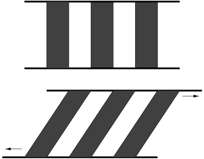
FIG. 3.: Increasing the energy of a system by shearing it.

The OJK theory also gives an explicit expression for the scaling form of the correlation function [8], which simply follows from equation (38) and from the scaling relations above

$$C_{OJK}(x,y;t)=\frac{2}{\pi}\sin^{-1}\left\{\frac{\langle m(1)m(2)\rangle}{\langle m(1)^{2}\rangle^{1/2}\langle m(2)^{2}\rangle^{1/2}}\right\}=\frac{2}{\pi}\sin^{-1}\left\{\exp\left[-\frac{1}{2}\left(\frac{s^{2}}{L_{\|}^{2}}+\frac{u^{2}}{L_{\bot}^{2}}\right)\right]\right\}\ .$$ (124)

It has been noted in [15] that in an unsheared, but anisotropic system the OJK form of the correlation function fits very well the numerical data. Note, however, that in the present case, unlike in[15], the scaling laws along the two main directions are radically different due to the shear, and therefore it is not a priori clear to what extent (124) is a good approximation to the scaling function $f$ in (114). On the other hand, we believe that the scaling form we find in (114) has a general validity. Finally, let us note the elliptic symmetry of the OJK correlation function, which could explain the partially correct results we obtained by approximating the domains with ellipses. The same will be true in three dimensions.

An important property of the result we have found is that the scale area of a domain $A(t)$ satisfies the following relation:

$$A(t)=L_{\|}L_{\bot}=2t\ ,$$ (125)

as in the case where no shear is present. As we are going to explain, there are topological reasons why in two dimensions relation (125) must be satisfied either with or without shear. Equation (125) is thus a necessary condition fulfilled by our result, which, by itself, clearly shows that the transverse growth must be depressed if the longitudinal one is enhanced.

Let us consider an isolated domain in two dimensions in the absence of shear. The rate of variation of the area enclosed in the loop is

$$\frac{dA(t)}{dt}=\oint dl\;v=-\oint dl\;\vec{\nabla}\cdot\vec{n}\ ,$$ (126)

where $v$ is the velocity of the interface and $\vec{\nabla}\cdot\vec{n}$ is the local curvature (see eq.(2)). By virtue of the Gauss-Bonnet theorem, the right-hand side of equation (126) is in two dimensions a topological invariant, and therefore independent of the shape of the domain.

When a shear is present, we have to add to the velocity due to the curvature the flow velocity $\vec{u}$ in the direction orthogonal to the interface. The right-hand side of equation (126) is thus corrected by the following term:

$$\oint dl\;\vec{n}\cdot\vec{u}=\int d^{2}x\;\vec{\nabla}\cdot\vec{u}=0\ ,$$ (127)

the final equality holding for any divergence-free shear flow. Equation (125), therefore, holds in two dimensions irrespective of the presence of the shear. It is interesting that the OJK approximation, in the self-consistent anisotropic version we have presented here, is able to capture this essential topological feature of phase ordering in two dimensions. Note also that the constant $2$ in relation (125) is exactly the same as one would obtain from the domain size in the absence of shear. We will find the same constant in the case of an oscillatory shear, as a further confirmation of the validity of our method.

V Oscillatory shear in two dimensions

The rather surprising results we have obtained in two dimensions could raise the question whether the OJK method, in the modified form we are using here, is actually suitable for studying the physics of a sheared system. Indeed, the skeptical reader may very well think that the shrinking of the transverse domains size, with the consequent increase in the total energy of the system, could be an artifact of the technique, rather than a genuine property of the model. On the other hand, as we have seen at the end of the last Section, our two-dimensional result satisfies the highly nontrivial topological relation on the growth of the scale area, eq. (125), supporting the validity of our findings. Therefore, to check how robust our method is, we test its compatibility with the two-dimensional topological constraint in a completely different situation. To this end we study in this Section the effect of an oscillatory shear on phase ordering in two dimensions.

It must be said that the case of oscillatory shear is interesting in itself. Indeed, a realistic experimental situation is very unlikely to involve an indefinite time-independent shear. More reasonably, a shear flow periodically depending on time, typically with some random modulation, is what we expect. Of course, real experiments with time independent shear can be performed (and we are proposing one in Section VIII): what we are saying is that a generalization of our calculation to a time-dependent oscillatory shear can shed some light on a more natural experimental setup.

We consider a sheared system with a velocity profile given by

$$\vec{u}=\gamma\,y\,G(t)\,\vec{e}_{x}\ ,$$ (128)

where the only assumption we make on the shear function $G(t)$ is that it is a periodic function with fundamental frequency $\omega$ and zero time average. One of the interesting aspects of the following calculation is that the results are to a great extent independent of the explicit form of $G(t)$. The derivation of the OJK equation is completely analogous to the one in Section II, and it follows simply from the obvious substitution

$$\gamma k_{x}\frac{\partial m(\vec{k},t)}{\partial k_{y}}\ \ \ \to\ \ \ \gamma G(t)k_{x}\frac{\partial m(\vec{k},t)}{\partial k_{y}}\ .$$ (129)

In order to solve the equations we have therefore to perform the change of variables (compare with (19))

$$q_{y}=k_{y}+\frac{\gamma}{\omega}g(t)k_{x}\ ,$$ (130)

with

$$g(t)\equiv\omega\int_{0}^{t}dt^{\prime}\ G(t^{\prime})\ .$$ (131)

Of course, for $G(t)=1$ we reproduce the time-independent shear case. All the equations of Section II can now be generalized to the oscillatory shear case by means of the following trivial substitution

$$\gamma t\ \ \to\ \ \frac{\gamma}{\omega}\,g(t)\ .$$ (132)

A critical issue to understand concerns the regime of the parameters, in particular time, that we have to consider. First of all, we cannot afford to have too high a frequency, otherwise there would be a delay in the response of the system to the shear. This means we must take the shearing frequency, $\omega$, much smaller than the shear rate, $\gamma$. On the other hand, we need to observe the system on time scales much larger than a period. Therefore, we will consider the following regime

$$\frac{1}{\gamma}\ll\frac{1}{\omega}\ll t\ ,$$ (133)

which implies

$$\alpha\equiv\frac{\gamma}{\omega}\gg 1\ .$$ (134)

Note that, in this way, we cannot recover from our final results the $\omega\to 0$ case, nor can we extrapolate to the $\omega\to\infty$ limit. On the other hand, the large parameter $\alpha$ will be useful for extracting the leading terms from our results.

Before going further, let us explain our general strategy. Due to the periodic shear, all our quantities will exhibit oscillations: some of them, like $D_{11}$, which is positive definite, will oscillate around a nonzero value, while others, like $D_{12}$, will oscillate around zero, due to the oscillation in the orientation of the domains. Given that all these quantities enter the time integrals in equations (27), a natural approach, for times much longer than the period, is to exploit their time-average: if $B(t)$ is an oscillatory quantity we write, to leading order for $t\to\infty$,

$$\int_{0}^{t}dt^{\prime}\ B(t^{\prime})\ t^{\prime n}\sim\bar{B}\ t^{n+1}\ ,$$ (135)

with

$$\bar{B}=\frac{\omega}{2\pi}\int_{0}^{\frac{2\pi}{\omega}}dt^{\prime}\ B(t^{\prime})\ .$$ (136)

In this way from equations (27) we get

$$R_{11}(t) = 4t\left\{1-\overline{D_{11}}+2\alpha\ \overline{gD_{12}}+\alpha^{2}\ \overline{g^{2}D_{11}}\right\}$$ (137)

$$R_{12}(t) = 4t\left\{-\overline{D_{12}}-\alpha\ \overline{gD_{11}}\right\}$$ (138)

$$R_{22}(t) = 4t\ \overline{D_{11}}\ .$$ (139)

Note the striking difference from the time-independent shear case: due to the oscillations the whole matrix $R_{ab}$ is now of order $t$, as it would be in the absence of shear. As mentioned above, we expect $D_{12}$ to oscillate around zero with the same period as $g$. Thus, in the equations above we can disregard terms like $\overline{D_{12}}$ and $\overline{gD_{11}}$, whose time average is zero. As a consequence, we have

$$R_{12}(t)=0\ ,$$ (140)

that is, the isotropy is restored at the level of the matrix $R_{ab}$. On the other hand, we have to keep mixed terms like $\overline{gD_{12}}$, because their time average will be nonzero. Using equations (34) we can now write

$$M_{11}(t) = 4t\left\{1-\overline{D_{11}}+2\alpha\ \overline{gD_{12}}+\alpha^{2}\ \overline{g^{2}D_{11}}+\alpha^{2}g^{2}(t)\ \overline{D_{11}}\right\}$$ (141)

$$M_{12}(t) = 4t\ \alpha\ g(t)\ \overline{D_{11}}$$ (142)

$$M_{22}(t) = 4t\ \overline{D_{11}}\ .$$ (143)

First of all note that, apart from the oscillation induced by the explicit presence of $g(t)$, the correlation matrix $M_{ab}$ is of order $t$, strongly suggesting that we will end up with a $t^{1/2}$ growth. On the other hand, $M_{12}\neq 0$, meaning that the system is still anisotropic, even though the anisotropy has zero time average.

From relation (134) and from equations (142), we have that $M_{11}\gg M_{12}\gg M_{22}$, and therefore the self-consistent equations (70), become

$$D_{11}(t) = \frac{M_{22}(t)+\sqrt{\sigma(t)}}{M_{11}(t)}$$ (144)

$$D_{12}(t) = -\frac{M_{12}(t)}{M_{11}(t)}\ .$$ (145)

As usual, we need a starting point to break into these equations and some physical considerations may help here. First, note that naively $M_{12}\sim L_{x}L_{y}\sim t$, from the topological relation (125). The second of equations (142) then suggests that $\overline{D_{11}}\sim 1/\alpha$. Secondly, from the form of the velocity profile, we have another naive relation, that is $x\sim\alpha\,y\,g(t)$. Thus, we expect that $-D_{12}\sim\theta\sim y/x\sim 1/\alpha$. We therefore make the following ansatz

$$D_{11}(t) = \frac{1}{\alpha}f(t)$$ (146)

$$-D_{12}(t) = \frac{1}{\alpha}h(t)\ ,$$ (147)

with $f(t)\geq 0$, while we expect $h$ to oscillate around zero. Both $f$ and $h$ must now be determined self-consistently. Inserting this ansatz into (142) and considering only the leading terms in $\alpha$, we have

$$M_{11}(t) = 4t\,\alpha[u+r\,g^{2}(t)]$$ (148)

$$M_{12}(t) = 4t\,g(t)r$$ (149)

$$M_{22}(t) = 4t\,\frac{r}{\alpha}$$ (150)

$$\sigma(t) = 16t^{2}\,ru\ ,$$ (151)

with the two constants $u$ and $r$ given by

$$r\equiv\overline{f}\ \ \ \ \ \ \ \ \ \ \ \ \ u\equiv\overline{g^{2}f}\ .$$ (152)

By inserting this form of $M_{ab}$ into equations (145), we find that the powers of $\alpha$ balance and we obtain two equations for the functions $f$ and $h$

$$f(t) = \frac{\sqrt{ru}}{u+rg^{2}(t)}$$ (153)

$$h(t) = \frac{rg(t)}{u+rg^{2}(t)}\ .$$ (154)

Averaging the first equation, we get

$$\sqrt{ru}=\Omega(r/u)\ ,$$ (155)

with

$$\Omega(x)=\overline{\left\{\frac{1}{1+xg^{2}(t)}\right\}}\ .$$ (156)

On the other hand, by multiplying the same equation by $g^{2}(t)$ and averaging again, we have

$$\sqrt{ru}=1-\Omega(r/u)\ ,$$ (157)

and therefore

$$\sqrt{ru}=\Omega(r/u)=1/2\ .$$ (158)

In order to compute the domain sizes we can use the same formulae as in Section IV, because we still have $\tau^{2}\simeq M_{11}^{2}\gg\sigma$. We obtain

$$L_{\parallel}(t) = \sqrt{\tau}=2t^{1/2}\ \sqrt{\frac{\gamma}{\omega}}\ \sqrt{u+rg^{2}(t)}$$ (159)

$$L_{\perp}(t) = \sqrt{\frac{\sigma}{\tau}}=2t^{1/2}\ \sqrt{\frac{\omega}{\gamma}}\ \frac{\sqrt{ru}}{\sqrt{u+rg^{2}(t)}}\ ,$$ (160)

and, happily, we find for the scale area

$$A(t)=L_{\parallel}(t)L_{\perp}(t)=4t\sqrt{ru}=2t\ ,$$ (161)

independent of the explicit form of the shear function $G(t)$. Note also that the factor $2$ in this formula is exactly the same as in the time-independent shear case and in the unsheared case. This is an important result, supporting the validity of our method for the study of the effect of shear in this type of system.

As expected, apart from the oscillations, the growth follows a $t^{1/2}$ law. The interesting thing is that both $L_{\parallel}$ and $L_{\perp}$ oscillate in time, but, as expected, with an opposite phase: when $g(t)$ has its maximum (i.e. at the maximum shear displacement), $L_{\parallel}$ is maximum and of course $L_{\perp}$ is minimum, because this is the point of maximum elongation of the domains. On the other hand, for $g(t)=0$ (i.e. zero shear displacement) $L_{\parallel}$ is minimum and $L_{\perp}$ maximum, but always with $L_{\parallel}\gg L_{\perp}$. We want to stress that this oscillatory dynamics is only deceptively simple. To better appreciate this fact we have to compute $L_{x}$ and $L_{y}$ (see Fig.2 and eq.(103)). These quantities read

$$L_{x}(t) = 2t^{1/2}\ \sqrt{\frac{\gamma}{\omega}}\ \sqrt{u}$$ (162)

$$L_{y}(t) = 2t^{1/2}\ \sqrt{\frac{\omega}{\gamma}}\frac{\sqrt{ru}}{\sqrt{u+rg^{2}(t)}}\ .$$ (163)

First of all, note that $L_{x}$, unlike $L_{y}$, does not oscillate in time, and this had to be expected from its very definition (see Fig.2). Secondly, note that for $g(t)=0$, we have $L_{x}=L_{\parallel}\gg L_{y}=L_{\perp}$: at the points of zero shear displacement the domains are very flat and large. Besides, we can compute the tilt angle $\theta$ from the eigenvectors of $M$, thus obtaining

$$\tan\theta=\frac{\omega}{\gamma}\ \frac{rg(t)}{u+rg^{2}(t)}\ .$$ (164)

We can see that $\theta$ is zero at the zero displacement point ($g(t)=0$), and increases with increasing displacement, up to a maximum, whose value decreases with increasing shear rate $\gamma$. This fact may seem counterintuitive, especially because in the case of a time-independent shear rate we have seen that the tilt angle was decreasing with time, while here it is increasing. However, there is no contradiction: the key point is that at $g(t)=0$ the domains are already very elongated, that is $L_{x}\gg L_{y}$, as an effect of the shear experienced in the former periods. We can better understand what happens by using the simple case of a linearly sheared ellipse (no growth), with initial axes $L_{x}$ and $L_{y}$, and $L_{x}\gg L_{y}$. The ellipse is described by the parametric equation

$$x = L_{x}\cos\phi+\gamma yt$$ (165)

$$y = L_{y}\sin\phi\ ,$$ (166)

with $\phi\in[0,2\pi]$. We can estimate the tilt angle by computing the ratio $y/x$ at the point where the $x$ displacement is maximum. This gives

$$\tan\theta=\frac{\gamma t}{\gamma^{2}t^{2}+L_{x}^{2}/L_{y}^{2}}\ .$$ (167)

This function has a maximum at

$$t_{\rm max}=\frac{1}{\gamma}\ \frac{L_{x}}{L_{y}}\ ,$$ (168)

and decreases asymptotically like $1/\gamma t$ for $t\to\infty$. In the case of time-independent shear rate, the initial condition $t=0$ has $L_{x}/L_{y}\sim 1$, and therefore the maximum of $\theta$ is quickly reached at $t_{\rm max}\sim 1/\gamma$, which is much smaller than the times we consider, $t\gg 1/\gamma$. For this reason, in the time region of interest the tilt angle monotonically decreases. In the oscillatory shear case, on the other hand, at the zero displacement point, $g=0$, we have $L_{x}/L_{y}\sim\gamma/\omega$ and thus $t_{\rm max}\sim 1/\omega$: the tilt angle therefore increases during the period of the oscillations, and this explains the apparent contradiction between the two cases.

From the tilt angle (164) we can compute the additional length scales $H_{x}$ and $H_{y}$ by using definition (107). We have

$$H_{x}(t) = 2t^{1/2}\ \sqrt{\frac{\gamma}{\omega}}\ \sqrt{u+rg^{2}(t)}$$ (169)

$$H_{y}(t) = 2t^{1/2}\sqrt{\frac{\omega}{\gamma}}\frac{rg(t)}{\sqrt{u+rg^{2}(t)}}\ .$$ (170)

Note that $H_{y}(t)$ is the only length scale to vanish at the zero displacement point. After the discussion above, the reason for this should now be clear.

In order to compute $r$ and $u$, we need to know the explicit form of $g(t)$, and therefore of $G(t)$. However, these are just numerical constants and the time evolution of the domain sizes is not affected by them. For the particularly simple case where

$$G(t)=\cos\omega t\ ,$$ (171)

the constants are

$$r=\frac{\sqrt{3}}{2}\ \ \ \ \ \ \ \ u=\frac{1}{2\sqrt{3}}\ .$$ (172)

VI Time independent shear in three dimensions

In dimension larger than two it becomes very difficult to explicitly compute the integrals in equations (48). Notwithstanding this, if we formulate a suitable ansatz for the elongation matrix $D_{ab}(t)$, we can then find $M_{ab}(t)$ from equations (27) and (34), and finally obtain a self-consistent relation for $D_{ab}(t)$ by an asymptotic evaluation for large times of the integrals in (48). In the present Section we will carry out this program for a time-independent shear rate.

First of all, we note that many of the terms in equations (27) can be estimated by means of the following reasonable ansatz:

$$D_{11}(t) \to 0\ \ \ ,\ \ \ t\to\infty$$ (173)

$$D_{12}(t) \sim -\frac{1}{\gamma t}\ .$$ (174)

Both these relations are also obtained in any dimension by the calculation of Section III. By inspection of equations (27) it is now clear that the key quantity needed to evaluate $R_{ab}(t)$, and thus $M_{ab}(t)$, is $[1-D_{22}(t)]$. We could be tempted to try an ansatz similar to the case $d=2$, by taking $[1-D_{22}(t)]\sim(\ln\gamma t)^{a_{1}}/t^{a_{2}}\to 0$, for $t\to\infty$. However, a careful analysis of the equations shows that this ansatz is not consistent. Therefore, the most natural thing to do is to assume that both $D_{22}(t)$ and $D_{33}(t)$ remain nonzero for $t\to\infty$, that is (according to the usual sum rule)

$$D_{22}(t) \to 1-K$$ (175)

$$D_{33}(t) \to K\ ,$$ (176)

and to fix self-consistently the value of the constant $K$. From equations (27), (34), (46) and (175) we have

$$M_{11}(t) = \frac{4}{3}K\gamma^{2}t^{3}$$ (177)

$$M_{12}(t) = 2K\gamma t^{2}$$ (178)

$$M_{22}(t) = 4Kt$$ (179)

$$M_{33}(t) = 4(1-K)\;t$$ (180)

$$\sigma(t) = \frac{4}{3}K^{2}\gamma^{2}t^{4}\ ,$$ (181)

at leading order for $t\to\infty$. Note that the explicit forms of $D_{11}(t)$ and $D_{12}(t)$ do not enter in $M_{ab}(t)$. Using relations (179) it is now possible to evaluate the asymptotic value of the integrals in equations (48) and get an equation for the constant $K$. In three dimensions equations (48) read

$$D_{22}(t) = \frac{1}{2}\sqrt{\sigma(t)M_{33}(t)}\int_{0}^{\infty}dy\;\frac{y^{2}+M_{11}(t)\,y+M_{11}(t)M_{33}(t)}{\{y^{3}+M_{11}(t)\,y^{2}+[M_{11}(t)M_{33}(t)+\sigma(t)]\;y+\sigma(t)M_{33}(t)\}^{3/2}}$$ (182)

$$D_{33}(t) = \frac{1}{2}\sqrt{\sigma(t)M_{33}(t)}\int_{0}^{\infty}dy\;\frac{y^{2}+M_{11}(t)\,y+\sigma(t)}{\{y^{3}+M_{11}(t)\,y^{2}+[M_{11}(t)M_{33}(t)+\sigma(t)]\;y+\sigma(t)M_{33}(t)\}^{3/2}}\ ,$$ (183)

where we have used the relation $M_{11}(t)\gg M_{22}(t)\sim M_{33}(t)$, according to (179). By performing the rescaling $y\to ty$ and by using relations (179) in the two integrals above, it is possible to see that in the limit $t\to\infty$ we can disregard the terms $y^{2}$ at the numerator and $y^{3}$ at the denominator. In this way we obtain

$$D_{22}(t) = \frac{\sqrt{\alpha}}{2}\int_{0}^{\infty}dy\;\frac{y+1-\beta}{(y^{2}+y+\alpha)^{3/2}}$$ (184)

$$D_{33}(t) = \frac{\sqrt{\alpha}}{2}\int_{0}^{\infty}dy\;\frac{y+\beta}{(y^{2}+y+\alpha)^{3/2}}\ ,$$ (185)

with

$$\alpha = \frac{4K(1-K)}{(4-3K)^{2}}$$ (186)

$$\beta = \frac{K}{4-3K}\ .$$ (187)

The fact that there is no time-dependence left in the right-hand sides of equations (185) shows that ansatz (174) and (175) give rise to a self-consistent solution for the three-dimensional case. Moreover, it is straightforward to check that sum rule (9) is satisfied. The integrals in (185) can now be easily performed and, by using relations (175), after some algebra we find

$$K=1/5\ .$$ (188)

A similar treatment of the integrals in (48) for $D_{11}(t)$ and $D_{12}(t)$ shows that,

$$D_{11}(t) \sim \frac{\ln(\gamma t)}{\gamma^{2}t^{2}}$$ (189)

$$D_{12}(t) \sim -\frac{1}{\gamma t}$$ (190)

consistent with ansatz (174). Let us note that relations (174), (175) and (179) are self-consistent in any dimension $d\geq 3$, as can be easily verified by using these relations in equations (48) and rescaling $y\to ty$ in the integrals. Our final result will therefore be qualitatively the same for any dimension $d\geq 3$ (for $d>3$ only numerical factors, such as the values of $K$ and the amplitudes in equations (192) below, are changed).

We can now compute the eigenvalues of the correlation matrix $M_{ab}(t)$, in order to find the sizes of the domains along the principal elongation axes. From (179) and (188), we have

$$L_{||}(t) = \frac{2}{\sqrt{15}}\;\ \gamma\;t^{3/2}$$ (191)

$$L_{\bot}(t) = \frac{1}{\sqrt{5}}\;\ t^{1/2}$$ (192)

$$L_{z}(t) = \frac{4}{\sqrt{5}}\;\ t^{1/2}\ ,$$ (193)

whose corresponding eigenvectors are

$$\vec{e}_{\|}=\left(1,\frac{3}{2\gamma t},0\right)\ \ ,\ \ \vec{e}_{\bot}=\left(-\frac{3}{2\gamma t},1,0\right)\ \ ,\ \ \vec{e}_{z}=\left(0,0,1\right)\ ,$$ (194)

where we recall that $L_{||}$ and $L_{\bot}$ are the larger and smaller orthogonal axes of the domain in the $(xy)$ plane, whereas $L_{z}$ is the axis of the domain in $z$ direction (or any direction orthogonal to the $(xy)$ plane, if $d>3$). The domain growth in dimension $d\geq 3$ is therefore the one we would expect on the basis of the simple scaling arguments given in Section II (see equations (15)): the growth exponent along the flow direction is augmented by one, whereas the others are left unchanged. Unlike the two-dimensional case, there are no topological restrictions on the product of the domain sizes, because the integral over the domain surface of the local curvature is not, in $d\neq 2$, a topological invariant.

As already anticipated, for $d=3$ standard scaling holds. Indeed, one can immediately check that

$$L_{\parallel}(t) \sim L_{x}(t)\sim H_{x}(t)$$ (195)

$$L_{\perp}(t) \sim L_{y}(t)\sim H_{y}(t)\ .$$ (196)

There is therefore no real difference between growth along the principal axes of the domains and growth in the $(xyz)$ directions, and the correlation function displays the simple asymptotic scaling form

$$C(x,y,z;t)=f\left(\frac{x}{L_{\|}},\frac{y}{L_{\bot}},\frac{z}{L_{z}}\right)\ .$$ (197)

According to the OJK theory [8], we have, for $t\to\infty$,

$$C_{OJK}(x,y,z;t)=\frac{2}{\pi}\sin^{-1}\left\{\exp\left[-\frac{1}{2}\left(\frac{(x+3y/2\gamma t)^{2}}{L_{\|}^{2}}+\frac{(y-3x/2\gamma t)^{2}}{L_{\bot}^{2}}+\frac{z^{2}}{L_{z}^{2}}\right)\right]\right\}\ .$$ (198)

In the scaling limit, where $x,y,z,t\to\infty$ with $x/L_{\|}$, $y/L_{\bot}$ and $z/L_{z}$ fixed, the term $3y/2\gamma t$ can be dropped, but the term $3x/2\gamma t$ cannot, and the OJK scaling function has ellipsoidal symmetry as expected.

As in two dimensions, we can compute the interfacial density by applying equation (119). The final result is

$$\rho(t)\sim\frac{1}{L_{\bot}}+\frac{L_{\bot}}{L_{\|}^{2}}\ ,$$ (199)

which shows that the energy density in the three dimensional case decreases in the standard way,

$$E(t)\sim t^{-1/2}\ .$$ (200)

VII Numerical simulations in two dimensions

In the present Section we will present some numerical simulations for a two-dimensional system subject to a time-independent uniform shear. We have considered a system of Ising spins on a lattice, governed by zero-temperature Monte Carlo dynamics. As in the rest of this paper, the shear flow is applied in the $x$ direction, according to the profile given by equation (12). From a practical point of view, we have sheared the system by shifting each row of spins by an amount proportional to the $y$ coordinate and to the time $\hat{t}$ (measured in Monte Carlo steps)

$$\Delta x(y,\hat{t})=y\,n_{s}(\hat{t})\ ,$$ (201)

where $n_{s}(\hat{t})$ is the number of discrete shear steps up to time $\hat{t}$. Of course, the discrete nature of the system is reflected in the discrete nature of the shearing process. To simulate a shear rate $\gamma$ (defined by $\Delta x_{\rm continuous}=\gamma y\hat{t})$) we require $n_{s}(\hat{t})={\rm Int}\,(\gamma\hat{t})$: After each $1/\gamma$ Monte-Carlo steps a discrete shear process, where each row moves one lattice spacing relative to the row below it, is applied. In the large-time limit, where $\hat{t}\gg 1/\gamma$, the system’s behavior should not be very different from that of a continuously sheared system.

We have to be careful in choosing the boundary conditions for a sheared system, because normal periodic boundary conditions would clearly be wrong. The idea is to replicate the original system infinitely many times on the $(x,y)$ plane and to shear each sub-system with respect to the others. In other words, if $(x,y)$ are the coordinates on the infinite plane, and $(i,j)$ are the coordinates on our numerical system, we have

$$i = {\rm Mod}_{N_{x}}(x+y\,n_{s}(\hat{t}))$$ (202)

$$j = {\rm Mod}_{N_{y}}(y)\ ,$$ (203)

where $N_{x}$ and $N_{y}$ are the sizes of the numerical system in the $x$ and $y$ directions, and the function ${\rm Mod}_{N}(z)$ is just the value of $z$ modulo $N$. Clearly, for $\hat{t}=0$ equations (203) reduce to standard periodic boundary conditions.

One of the main difficulties in simulating a system subject to a shear is that the domains grow very quickly in the direction of the flow, soon reaching a size comparable with the size of the system. On the other hand, as we have seen, we expect the growth to be highly depressed in the transverse direction. Thus, the most reasonable thing to do is to take $N_{x}\gg N_{y}$, in order to reduce as much as possible finite size effects. In all our simulation we have taken $N_{x}=20000$ and $N_{y}=100$. As we shall see, even for our longest times, the domains are much smaller than the size of the system in both directions. A possible proposal in order to reduce the finite size effects due to the shear-induced elongation of the domains is to work at very low $\gamma$. However, all our results hold in the limit $L_{x}\gg L_{y}$: if we decrease the shear we will have to wait for a longer time to enter the asymptotic regime of interest, and thus we will still have the problem of long domains compared to the system size. There is, therefore, no easy way out of this situation and we had to tune our parameters to take this problem into consideration. For this reason we run our simulations for only one value of the shear rate, namely $\gamma=1/4$: in order to study the dependence of all the observables on the shear rate we would have to consider values of $\gamma$ far from the suitable numerical domain.

The first thing we want to check is the behavior of the length scales $L_{x}(t)$ and $L_{y}(t)$. As we have seen, $x$ and $y$ are not the correct scaling axes, but we want to test our prediction for $L_{x}$ and $L_{y}$ against the naive expectation of equation (15). Indeed, it must be remembered that this naive scaling is also the one found in the case of conserved dynamics in the limit of infinite dimension of the field [9]. We recall our analytic prediction

$$L_{x}(t) \sim \frac{\sqrt{\gamma}\,t}{(\ln\gamma t)^{1/4}}$$ (204)

$$L_{y}(t) \sim \frac{1}{\sqrt{\gamma}\,(\ln\gamma t)^{1/4}}\sim L_{\perp}(t)\ .$$ (205)

Note that $L_{y}$ is, at the leading order, equal to $L_{\perp}$, and therefore we can limit ourselves to measure the former. This is important, because a numerical measure of $L_{\perp}$ would be very difficult: the domain size in the perpendicular direction is very small and for long times this direction passes through very few lattice sites, such that practically there are no points where the correlation function is different from zero. This problem does not exists for the correlation in the $x$, $y$ and parallel direction. In order to extract the the domain scale at a given time we have performed a fit of the correlation function to the OJK form and have located the point where the fit is equal to $1/e$. We have checked that the behavior of the domain size with time is almost entirely insensitive to the particular fit we use. Numerically, we do not expect to be able to detect the logarithmic corrections in (205), so our goal is to check the leading behavior $L_{x}\sim t$ and $L_{y}\sim O(1)$. Our results are shown in Fig.4.

FIG. 4.: The domain sizes in the $x$ and $y$ direction as a function of time. The full line is a power fit giving $L_{x}\sim t^{1.02}$. The dashed line is $L_{x}^{\rm naive}\sim t^{3/2}$, and the dotted line is $L_{y}^{\rm naive}\sim t^{1/2}$, for a comparison. In both cases, the data are averaged over $5$ samples.

As we can see, $L_{x}$ is definitely not growing like $t^{3/2}$. A power fit gives

$$L_{x}(t)\sim t^{1.02}\ .$$ (206)

Furthermore, $L_{y}$ is, on this scale, compatible with a constant, and is certainly not growing like $t^{1/2}$. Both $L_{x}(t)$ and $L_{y}(t)$ have the expected behavior, apart from the logarithmic corrections, and the naive exponents $3/2$ and $1/2$ are clearly not correct.

The value of $L_{y}$ is very small and in order to have a better idea of the fast decay of the correlation in the $y$ direction, we plot in Fig.5 the correlation function and the OJK fit for a given fixed value of the time. Note that actually the correlation vanishes on average after six lattice spacings.

The next important quantity we want to measure is the energy. From relation (123) we can see that $E(t)$ is a direct measure of $L_{\perp}(t)$. Note that the relation between $E$ and $L_{\perp}$ is, at leading order, completely independent on the OJK approximation we are using: indeed, the simple assumption $L_{\parallel}\gg L_{\perp}$ is sufficient to conclude that, at leading order, $E\sim 1/L_{\perp}$. However, we stress that the condition $L_{\parallel}\gg L_{\perp}$ is only satisfied for large times (see Fig.4). In Fig.6 we plot the energy as a function of time, both for the sheared and the unsheared case. We see that, after an initial drop in the time regime where we do not expect relation (123) to hold, the energy becomes compatible with a constant on this scale. The difference with the unsheared case is striking. In the inset of this figure we show a magnification of the last part of the curve for the sheared case: it is encouraging to see that, despite the significantly large error bars, an increase in the energy for very large times is clearly visible, compatible with our analytic prediction

$$E(t)\sim\sqrt{\gamma}\,(\ln\gamma t)^{1/4}\ .$$ (207)

However, we stress that longer simulational times and larger system sizes are necessary to test this prediction (in particular, the power of the logarithm) more carefully.

FIG. 5.: Correlation function in the $y$ direction as a function of $y$, for $\hat{t}=144$. The symbols are the numerical data for $5$ samples; the full line is the OJK fit.

FIG. 6.: The energy as a function of time in the sheared case ($\gamma=1/4$), averaged over 41 samples, and the unsheared case ($\gamma=0$) averaged over 5 samples. The full line is a power fit for the unsheared case, giving $E_{\rm un}\sim t^{-0.51}$. The horizontal broken line is a guide to the eye. Inset: energy in the sheared case as a function of time (magnification).

The last quantity we measure is $L_{\parallel}(t)$, whose form (101) differs from that of $L_{x}(t)$ only by a logarithmic correction. In Fig.7 we plot $L_{\parallel}$ as a function of the time. Even if slightly faster, the growth of the domains in the parallel direction is compatible with $t$. Indeed, a power fit gives

$$L_{\parallel}(t)\sim t^{1.14}\ .$$ (208)

Not surprisingly, at a simulational level we are unable to detect any significant difference between the growth of $L_{x}$ and $L_{\parallel}$.

FIG. 7.: Domain size $L_{\parallel}$ as a function of time, averaged over 10 samples. The full line is a power fit, giving $L_{\parallel}(t)\sim t^{1.14}$.

Summarizing, we can say that, up to the simulational times we were able to reach, numerical data are largely compatible with our theoretical results. In particular, the nontrivial leading behavior of $L_{x}(t)$, $L_{y}(t)$ and $L_{\parallel}(t)$ are correctly reproduced, while the naive expectations for the domain growth is sharply ruled out by the simulations. Note that, of course, a longer simulational time would be desirable, especially to check whether the curve of the energy develops a well defined minimum and eventually starts increasing as $(\ln t)^{1/4}$. Unfortunately, as we have seen, the high values of $L_{x}$ and $L_{\parallel}$ make this impossible with the system sizes we were able to reach, otherwise finite size effects would heavily come into play. Also for this reason, in the next Section we propose a real experimental test of our analytical results.

VIII An experimental test of the two-dimensional results

Theoretical and numerical results on nonconserved two-dimensional coarsening dynamics can be experimentally tested by means of thin films of uniaxial twisted nematic liquid crystal (TNLC) subjected to rapid thermal quenches. Since the classic experiments of Orihara, Ishibashi and Nagaya [10], showing that a dynamical scaling compatible with the law $L(t)\sim t^{1/2}$ actually takes place in this system [16], many other workers have successfully tested numerical and theoretical results on nonconserved coarsening in TNLC [11]. In particular, let us note that this kind of system seems to be particularly suitable for testing our analytic calculation: indeed, it has been shown in [10] that the scaling function describing the two-dimensional coarsening dynamics in TNLC is very well approximated by the analytic expression given by the OJK theory [8]. Moreover, it has been explicitly checked [10] that the Allen-Cahn equation (2), describing the motion of an interface due to its curvature, holds to a very good degree of accuracy for TNLC. Our aim is to describe in this Section the basic experimental setup for TNLC and to propose a shear experiment on such systems, in order to test our nonstandard two-dimensional results in the case of simple, time-independent shear.

A typical TNLC cell is obtained by confining the sample of nematic liquid crystal between two glass plates, previously prepared by rubbing them in two mutually perpendicular directions. In this way the orientations of the crystal molecules belonging to the two layers close to the plates have a relative rotation of $\pi/2$. At high temperature, in the isotropic phase, the boundary conditions only affect the system close to the boundaries, but when the crystal is quenched below the transition temperature (also called the clearing point), deep into the nematic phase, the alignment of the molecules with the boundary conditions on the plates extends into the bulk. In this way two different states appear, corresponding to the possibility of the molecules to rotate between the directions imposed by the two boundary plates in either a clockwise or an anti-clockwise sense. In other words, after the quench the TNLC cell develops two equivalent states, which we may call left-handed and right-handed. Domains of the two states are separated by disclination lines [10], defined as the points where the sense of rotation changes sign. The system is effectively two-dimensional and the dynamics of the left and right-handed domains is very well described by nonconserved coarsening dynamics.

In order to reproduce the situation studied in the present paper, it is necessary to shear the TNLC cell in a such a way that the shear direction is parallel to the two plates (the flow direction is of course parallel to them). Namely, the mutual orientation of the two plates must not be changed in the experiment, while the orthogonal walls must be moved in order to create the shear. In this way our $(xy)$ plane would be parallel to the rubbed glass plates.

Given that a vital condition for testing our asymptotic results, in the case of time-independent shear, is the possibility to shear the system for a long time, it seem to us that a linear geometry is probably unsuitable for such an experiment. On the contrary, a circular setup may be more convenient: by taking two circular glass plates, rubbed tangentially and radially, it is possible to create a cell whose wall, orthogonal to the plates, can now be rotated indefinitely. In order to create the shear it is necessary to place a fixed cylinder at the center of the system. In this way the material in contact with this cylinder is stationary, while the layers close to the outer walls move with a given tangential velocity $u_{0}$, creating a velocity profile given by

$$u(r)=\frac{u_{0}R_{0}}{R_{0}^{2}-R_{c}^{2}}\,\left(r-\frac{R_{c}^{2}}{r}\right)\ \ \ ,\ \ \ R_{c}<r<R_{0}\ ,$$ (209)

where $R_{0}$ and $R_{c}$ are the radius of the cell and of the internal cylinder, respectively. If $R_{c}-R_{0}\ll R_{0}$, it is possible to produce a flow identical to the one studied in the present work and to study the long time dynamics of the domains under shear. Indeed, by setting $r=R_{c}+y$, we have

$$u(y)=\frac{2u_{0}R_{0}}{R_{0}^{2}-R_{c}^{2}}\ y\ \ \ ,\ \ \ y\ll R_{c}\ ,$$ (210)

to be compared with relation (12).

Finally, testing our results in the case of oscillatory shear should be easier from the experimental point of view, since the periodicity of the shear function allows for the simpler linear geometry. As we have seen, the main growth follows a $t^{1/2}$ law, modulated by some oscillations in the longitudinal direction. In particular, it should not be difficult to test whether the ratio of perpendicular and parallel domain sizes satisfies the relation

$$\frac{L_{\perp}}{L_{\parallel}}\sim\frac{\omega}{\gamma}\ ,$$ (211)

in the regime where $\gamma\gg\omega$.

IX Conclusions

In this paper we have analytically studied the effect of a shear flow on phase ordering, for a statistical system with nonconserved scalar order parameter. We have developed a self-consistent anisotropic version of the OJK approximation, by means of which we have calculated the growth exponents for time-independent shear in two and three dimensions (relations (101) and (192)), and we have found the scaling form of the equal-time two-point correlation function in both cases (relations (114), (116) and (197)). While for $d=3$ our results are consistent with some simple scaling arguments and with the results obtained for conserved dynamics in the limit of large dimension $N$ of the order parameter, in $d=2$ we find that domain growth is so heavily affected by the shear, that the domains experience a narrowing which in principle makes their thickness vanish in the limit $t\to\infty$. However, as we have pointed out, our calculation is likely to break down for very long times, when the interface and the domain thickness are of the same order. What happens beyond this stage is still unclear to us: it is possible that a time-dependent steady state develops, with very narrow domains coalescing and giving rise to new thicker domains, which start narrowing again. Another possible scenario is that when $L_{\bot}\sim\xi$ domains start breaking and stretching again, giving rise to a steady state like the one depicted in [5]. Further work is needed to clarify this point and it is to be hoped that experiments on twisted nematic liquid crystals, as described in the last Section, will lead to a deeper understanding of this problem.

We have also studied the case of an oscillatory shear in two dimensions, finding a standard $t^{1/2}$ growth, modulated by periodic oscillations which occur in opposition of phase for the parallel and perpendicular direction. Interestingly enough, all our results in this case are largely independent on the particular form of the shear rate oscillations.

It is important to note that, in two dimensions, our results satisfy the topological constraint on the growth of the scale area, both in the time-independent and oscillatory case. This fact, together with the results of our numerical simulations, strongly support the validity of our method in the study of coarsening systems under shear.

Of course, it would be very interesting to know whether some of our results (in particular in dimension two) are preserved for conserved dynamics, which is the relevant case for describing spinodal decomposition in binary fluids. Unfortunately, the OJK approximation cannot be used in this case, since the very starting point, the Allen-Cahn equation for the interface motion, does not hold when the order parameter is conserved. It is therefore still unclear how to go beyond the large-$N$ limit in the context of spinodal decomposition under shear.

- [1] See A.J. Bray, Adv. Phys. 43, 357 (1994), and references therein.
- [2] See A. Onuki, J. Phys.: Condens. Matter 9, 6119 (1997), and references therein.
- [3] C. K. Chan, F. Perrot, and D. Beysens, Phys. Rev. A 43, 1826 (1991); A. H. Krall, J. V. Sengers, and K. Hamano, Phys. Rev. Lett. 69, 1963 (1992); T. Hashimoto, K. Matsuzaka, E. Moses, and A. Onuki, Phys. Rev. Lett. 74, 126 (1995); J. Läuger, C. Laubner, and W. Gronski, Phys. Rev. Lett. 75, 3576 (1995).
- [4] D. H. Rothman, Phys. Rev. Lett. 65, 3305 (1990); P. Padilla and S. Toxvaerd, J. Chem. Phys. 106, 2342 (1997); A. J. Wagner and J. M. Yeomans, Phys. Rev. E 59, 4366 (1999).
- [5] T. Ohta, H. Nozaki, and M. Doi, Phys. Lett. A 145, 304 (1990); J. Chem. Phys. 93, 2664 (1991).
- [6] For a discussion of domain growth saturation and finite size effects, see M. E. Cates, V. M. Kendon, P. Bladon, and J.-C. Desplat, Faraday Discuss. 112, 1 (1999).
- [7] P.C. Hohenberg, and B.I. Halperin, Rev. Mod. Phys. 49, 435 (1977).
- [8] T. Ohta, D. Jasnow, and K. Kawasaki, Phys. Rev. Lett. 49, 1223 (1982).
- [9] F. Corberi, G. Gonnella, and A. Lamura, Phys. Rev. Lett. 81, 3852 (1998); N. P. Rapapa and A. J. Bray, Phys. Rev. Lett. 83, 3856 (1999).
- [10] H. Orihara and Y. Ishibashi, J. Phys. Soc. Jpn. 55, 2151 (1986); T. Nagaya, H. Orihara and Y. Ishibashi, J. Phys. Soc. Jpn. 56, 3086 (1987).
- [11] I. Chuang, N. Turok, and B. Yurke, Phys. Rev. Lett. 66, 2472 (1991); R. Snyder, A.N. Pargellis, P.A. Graham, and B. Yurke, Phys. Rev. A 45, R2169 (1992); N.Mason, A.N. Pargellis, and B.Yurke, Phys. Rev. Lett. 70, 190 (1993); B.Yurke, A.N. Pargellis, S.N. Majumdar, and C. Sire, Phys. Rev. E 56, R40 (1997).
- [12] A. J. Bray and A. Cavagna, cond-mat/0001299 (2000).
- [13] L.D. Landau and I.M. Khalatnikov, Dokl. Akad. Nauk SSSR 96, 469 (1954).
- [14] S. M. Allen and J. W. Cahn, Acta Metall. 27, 1085 (1979).
- [15] E. N. M. Cirillo, G. Gonnella and S. Stramaglia, Phys. Rev. E 56, 5065 (1997).
- [16] The actual value of the dynamical exponent found by Orihara and Ishibashi was .