Single-hole dynamics in dimerized and frustrated spin-chains

Abstract

We present a unified account for the coupled single-hole- and spin-dynamics in the spin-gap phase of dimerized and frustrated spin-chains and two-leg spin ladders. Based on the strong dimer-limit of a one-dimensional $t_{1,2,3}$-$J_{1,2,3}$-model a diagrammatic approach is presented which employs a mapping of the spin-Hamiltonian onto a pseudo-fermion bond-boson model. Results for the single-hole spectrum are detailed. A finite quasi-particle weight is observed and studied for a variety of system parameters. A comparison with existing exact diagonalization data is performed and good agreement is found.

I Introduction

Unconventional quantum-magnetism in low-dimensional transition-metal compounds has received considerable interest recently due to the discovery of numerous novel materials with spin-$\frac{1}{2}$ moments arranged in chain, ladder, and depleted planar structures. Among these compounds are antiferromagnetic chain-systems which are intrinsically dimerized, in particular, (VO)₂P₂O₇ [1], CuWO₄ [2], and Cu(NO₃)${}_{2}\cdot 2.5$H₂O [3]. Moreover, quasi-one-dimensional (1D) materials have been discovered which display a temperature dependent dimerization, eg. CuGeO₃ [4] and $\alpha^{\prime}$-NaV₂O₅ [5] where the former is the first inorganic spin-Peierls chain [6] and magnetically frustrated [7, 8] while the latter is a $\frac{1}{4}$-filled two-leg ladder [9]. Spin-ladders, both inorganic, eg. SrCu₂O₃ [10] and CaV₂O₅ [11] as well as organic, eg. Cu₂(C₂H₁₂N₂)₂Cl₄ [12] have been investigated. Quite recently SrCu₂(BO₃)₂ [13, 14] has been shown to realize the two-dimensional (2D) version [15] of the 1D frustrated Majumdar-Ghosh model [16].

In contrast to conventional 1D spin-chain materials, eg. Sr₂CuO₃ and SrCuO₂ [17, 18], which display algebraic, almost long-range, spin-correlations and gap-less magnetic excitations the new materials are spin-liquids (or dimer-solids) with short-range singlet correlations and a gap in the spin spectrum. The spin-gap phenomenon has been attributed to dimerization [6, 19] and frustration [16, 20, 21] in chain-systems, and it can be interpreted accordingly in ladders due to their topological equivalence to frustrated and dimerized chains [22, 23].

Apart from magnetic excitations the dynamics of electronic carriers doped into quasi-1D spin-liquids is of interest, in particular because of the discovery of superconductivity [24] in the two-leg ladder-compound Sr_14-xCa_xCu₂₄O₄₁ [25]. Important progress has been achieved regarding the pairing correlations and the phase diagram of spin-ladders [23]. However, only a restricted set of primarily numerical studies [26, 27, 28, 29, 30, 31, 32, 33] has focused on the spectral properties of single-hole excitations in quasi-1D spin-liquids at low doping. In this regime, and due to the spin-gap, a quasi-particle picture [34], rather than a Luttinger-liquid description [35], is believed to be relevant at low energy scales [27].

In this paper we detail a theory of single-hole excitations at half-filling for a dimerized and frustrated spin-chain. Particular emphasis will be on the coupling between spin and charge degrees of freedom. The paper is organized as follows: first we introduce the $t_{1,2,3}$-$J_{1,2,3}$-model for the dimerized and frustrated spin system. Second we summarize a bond-boson-method to evaluate the spin-excitations at half filling starting from the strong dimer limit. Third, we map the $t_{1,2,3}$-$J_{1,2,3}$-model in the single-hole sector onto a coupled boson-fermion-model. Next, the single-hole excitations of the latter model are evaluated by a selfconsistent diagrammatic technique. Finally we present results for the spectral properties of the single hole, both for ladders and chains, and compare our findings to existing numerical analysis of finite systems.

II The $t_{1,2,3}$-$J_{1,2,3}$-model

For the remainder of this work we focus on systems which are of a Mott- or charge-transfer type of insulator at half filling and allow for an approximate mapping to a $t$-$J$-model. To describe the case of either dimerization and frustration of the magnetic exchange coupling along the chain or the topology of a two-leg ladder we invoke a $t$-$J$-model which includes hopping- and exchange-integrals up to third-nearest-neighbors (NNN), i.e. $t_{1,2,3}$ and $J_{1,2,3}$, as shown in figure 1.

FIG. 1.: $t_{1,2,3}$-$J_{1,2,3}$-model. $n$ labels the dimer bonds. 1 and 2 refer to non-equivalent sites per unit cell.

Depending on the case of a ladder or a chain the real-space structure of the system is either identical to that of figure 1 with $J_{2}=t_{2}=0$ or can be obtained by deforming the figure such as to place sites $2,n$ half-way in-between sites $1,n$ and $1,n+1$. The Hamiltonian reads

$$H= H_{t}+H_{J}$$ (1)

$$H_{J}= J_{1}\sum_{n}{\bf S}_{1,n}{\bf S}_{2,n}+J_{2}\sum_{n}{\bf S}_{2,n}{\bf S}_{1,n+1}$$ (4)

$$+J_{3}\sum_{i}({\bf S}_{1,n}{\bf S}_{1,n+1}+{\bf S}_{2,n}{\bf S}_{2,n+1}),$$

$$H_{t}= -t_{1}\sum_{n,\sigma}\hat{c}_{1,n,\sigma}^{\dagger}\hat{c}_{2,n,\sigma}^{\phantom{\dagger}}-t_{2}\sum_{n,\sigma}\hat{c}_{2,n,\sigma}^{\dagger}\hat{c}_{1,n+1,\sigma}^{\phantom{\dagger}}$$ (6)

$$-t_{3}\sum_{n,\sigma}(\hat{c}_{1,n\sigma}^{\dagger}\hat{c}_{1,n+1,\sigma}^{\phantom{\dagger}}+\hat{c}_{2,n\sigma}^{\dagger}\hat{c}_{2,n+1,\sigma}^{\phantom{\dagger}})+h.c.$$

where ${\bf S}_{i,n}$ are spin-1/2 operators on site $i$ of dimer-bond $n$ and $\hat{c}_{i,n,\sigma}^{(\dagger)}=[c_{i,n,\sigma}(1-n_{i,n,-\sigma})]^{(\dagger)}$ are projected fermion-operators of spin $\sigma$ on site $i,n$. Dimerization and frustration of the spin-system is expressed via the parameters $\delta$ and $\alpha$ where $J_{1(2)}=J_{0}(1+(-)\delta)$ and $\alpha=J_{3}/J_{0}$. Similarly the hopping integrals are related through $t_{1(2)}=t_{0}(1+(-)\tilde{\delta})$ and $\tilde{\alpha}=t_{3}/t_{0}$. Ladders are characterized by $\delta=\tilde{\delta}=1$. Regarding the spin-part, i.e. $H_{J}$, the ground state is known to be a product-state of singlets located on the dimer-bonds for $\alpha$ and $\delta$ on the disorder-line [16, 15] $\delta=1-2\alpha$, moreover, the spin-spectrum is gap-less only at $\delta=0$ and $0\leq\alpha<\alpha_{C}$ with $\alpha_{C}\simeq 0.2411$ [20, 21]. For magnetic couplings which are mediated by super-exchange and for systems with only a single relevant on-site Coulomb-energy scale we expect that $(1+\tilde{\delta})^{2}\sim(1+\delta)$ and $\tilde{\alpha}^{2}\sim\alpha$ for $|\delta,\alpha|\ll 1$.

III Undoped spin-system

The spin-part, i.e. $H_{J}$, of Hamiltonian (1) allows for a mapping onto a model of hard-core ’bond’-bosons originally employed in the context of the 2D Heisenberg-model for the high-T_C cuprates [36]. Here we briefly restate the essential features of this mapping. Consider any two spin–1/2 operators ${\bf S}_{1,n}$ and ${\bf S}_{2,n}$. The eigenstates of the related total spin are a singlet and three triplets These can be created out of a vacuum $\left|0\right>$ by applying the bosonic operators $s_{n}^{\dagger}$ and $t_{\alpha,n}^{\dagger}$ with $\alpha=x,y,z$

$$s_{n}^{\dagger}|0\rangle=\frac{1}{\sqrt{2}}\left(|\!\uparrow\downarrow\rangle-|\!\downarrow\uparrow\rangle\right)_{n}$$ (7)

$$t_{x,n}^{\dagger}|0\rangle=\frac{-1}{\sqrt{2}}\left(|\!\uparrow\uparrow\rangle-|\!\downarrow\downarrow\rangle\right)_{n}$$ (8)

$$t_{y,n}^{\dagger}|0\rangle=\frac{i}{\sqrt{2}}\left(|\!\uparrow\uparrow\rangle+|\!\downarrow\downarrow\rangle\right)_{n}$$ (9)

$$t_{z,n}^{\dagger}|0\rangle=\frac{1}{\sqrt{2}}\left(|\!\uparrow\downarrow\rangle+|\!\downarrow\uparrow\rangle\right)_{n}$$ (10)

where the first (second) entry in the kets refers to site 1(2) on dimer $n$ of fig. 1. On each site we have $[s,s_{\phantom{\alpha}}^{\dagger}]=1$, $[s_{\phantom{\alpha}}^{(\dagger)},t_{\alpha}^{(\dagger)}]=0$, and $[t_{\alpha}^{\phantom{(\dagger)}},t_{\beta}^{\dagger}]=\delta_{\alpha\beta}$. The action of ${\bf S}_{1,n}$ and ${\bf S}_{2,n}$ in this space leads to the representation

$$S^{\alpha}_{{}^{1}_{2},n}=\frac{1}{2}(\pm s_{n}^{\dagger}t_{\alpha,n}^{\phantom{\dagger}}\pm t_{\alpha,n}^{\dagger}s_{n}-i\epsilon_{\alpha\beta\gamma}^{\phantom{\dagger}}t^{\dagger}_{\beta,n}t_{\gamma,n}^{\phantom{\dagger}}).$$ (11)

Here $\varepsilon_{\alpha\beta\gamma}$ is the Levi–Civita symbol and a summation over repeated indices is implied hereafter. The upper(lower) subscript on the lhs. of (11) refer to upper(lower) sign on the rhs.. The bosonic Hilbert space has to be restricted to the physical Hilbert space, i.e. to either one singlet or one triplet per site, by the constraint

$$s_{n}^{\dagger}s_{n}^{\phantom{\dagger}}+t_{\alpha,n}^{\dagger}t_{\alpha,n}^{\phantom{\dagger}}=1$$ (12)

The representation (11) can be inserted into (4) yielding an interacting bose-gas Hamiltonian accompanied by the constraint (12) [36]. This Hamiltonian is diagonal intra-dimer-wise and contains two-particle interactions which are only of inter-dimer type. At the point of complete dimerization, i.e., $\delta=1$ and $\alpha=0$, the inter-dimer interactions vanish leaving a sum of purely local dimer Hamiltonians, each of which has a singlet ground state. This renders the global ground-state a product of singlets localized on the dimers with the excitations being a set of 3^N-fold degenerate triplets. Off the dimer-point the inter-dimer interactions can be treated approximately by a linearized Holstein-Primakoff (LHP) approach, details of which can be found in the literature [37, 38, 39, 40]. The LHP method retains spin-rotational invariance and reduces $H_{J}$ to a set of three degenerate massive magnons

$$H_{J}=\sum_{k}\omega_{k}\gamma_{\alpha,k}^{\dagger}\gamma_{\alpha,k}^{\phantom{\dagger}}+\mbox{const.}$$ (13)

with

$$t_{\alpha,k}^{\dagger} = u_{k}\gamma_{\alpha,k}^{\dagger}+v_{k}\gamma_{\alpha,-k}^{\phantom{\dagger}},$$ (14)

$$\omega_{k} = J_{1}\sqrt{1+2e_{k}}$$ (15)

$$e_{k} = \frac{2J_{3}-J_{2}}{2J_{1}}\cos{k}$$ (16)

$$u[v]_{k}^{2} = \frac{1}{2}\left(\frac{J_{1}(1+e_{k})}{\omega_{k}}+[-]1\right)$$ (17)

The ’$[]$’-bracketed sign on the rhs. in (17) refers to the quantity $v$ on the lhs.. The spin-gap $\Delta=\min\{\omega_{k}\}$ resides at $k=\pi(0)$ with $\Delta=\sqrt{J_{1}^{2}-(+)J_{1}(2J_{3}-J_{2})}$ for $2J_{3}>(<)J_{2}$. Note that because of (14) the ground state $|D\rangle$, which is defined by $\gamma_{\alpha,k}|D\rangle=0$, contains quantum-fluctuations beyond a pure singlet product-state.

To leading order the dispersion $\omega_{k}$ is identical to perturbative expansions, both, for chains [41, 42] and ladders [43, 44] and it has been applied to model inelastic neutron scattering (INS) data for CuGeO₃ [40] and $\alpha^{\prime}$-NaV₂O₅ [45]. Beyond the LHP approach triplet-interactions lead to a renormalization of $\omega_{k}$ and to the formation of multi-magnon bound states [46, 47, 48]. Moreover the constraint (12), although a hardcore repulsion, has been considered perturbatively relying on the case of low triplet-density at $\Delta/J\ll 1$ [46, 47, 49]. These renormalizations of the triplet dispersion will be discarded in our evaluation of the single-hole spectra, in particular since their dominant effects can be accounted for semi-phenomenologically by adjusting the size of the LHP spin-gap. This is of significance when comparing single-hole spectra to numerical studies, as in section VII.

IV Single-hole Hamiltonian

In this section we map the $t_{1,2,3}$-$J_{1,2,3}$-Hamiltonian of (1-6) in the single-hole sector onto a model of pseudo-fermions interacting with the bond-bosons. To this end we note that a dimer-bond occupied by a single hole can be labeled by introducing an additional pseudo-fermion (holon). I.e., instead of the bond being in one of the states given by (10) it can also be in the state

$$a_{j,n,\sigma}^{\dagger}|0\rangle=|j\sigma\rangle_{n}$$ (18)

where the l.h.s. denotes the vacuum, i.e. $|0\rangle$, with a single dimer-bond at site $n$ in a one-hole state of spin $\sigma$ with $j=1,2$ referring to the two positions available to the hole on the bond. The operators $a^{\phantom{\dagger}}_{j,i,\sigma}$ are required to obey fermionic anticommutation relations. In the single-hole sector each dimer-bond can only be in exactly one of the states given by (10) or (18). Therefore an extended hard-core constraint has to be satisfied

$$s_{i}^{\dagger}s_{i}^{\phantom{\dagger}}+t_{\alpha,i}^{\dagger}t_{\alpha,i}^{\phantom{\dagger}}+\sum_{j=1,2}a_{j,i,\sigma}^{\dagger}a_{j,i,\sigma}^{\phantom{\dagger}}=1$$ (19)

with a summation over repeated spin-indices implied. Creation of a single physical hole in the (half-filled) ground state $|D\rangle$ of the spin-system is achieved by applying the two-particle operator

$$\hat{c}_{j,n,\sigma}= \frac{p_{j}}{\sqrt{2}}[a_{\overline{j},n,\overline{\sigma}}^{\dagger}(p_{j}p_{\sigma}s_{n}^{\phantom{\dagger}}+t_{z,n}^{\phantom{\dagger}})$$ (21)

$$+a_{\overline{j},n,\sigma}^{\dagger}(p_{\overline{\sigma}}t_{x,n}^{\phantom{\dagger}}+it_{y,n})^{\phantom{\dagger}}]$$

where $p_{j}=+(-)$, $\overline{j}=2(1)$ for $j=1(2)$ and $p_{\sigma}=+(-)$, $\overline{\sigma}=\downarrow(\uparrow)$ for $\sigma=\uparrow(\downarrow)$. In terms of the previous equation the creation of a physical hole can be interpreted has the removal of a spin-dimer followed by the creation of dimer hole-state, where the particular linear combination of the $a_{j,n,\sigma}^{\dagger}$, $s_{n}^{\phantom{\dagger}}$, and $t_{\alpha,n}^{\phantom{\dagger}}$ operators on the r.h.s. ensures that the total spin is $S=1/2$ and $S_{z}=\pm 1/2$. Using the constraint (19) it is straightforward to show, that the r.h.s. of (21) indeed satisfies the usual Hubbard-operator algebra.

Inserting (21) into (1-6) we have to distinguish between various cases, i.e., (i) intra-dimer hopping, (ii) inter-dimer hopping, and (iii) exchange-scattering. Inter-dimer hopping can be either spin-diagonal or accompanied by spin-flip scattering. This includes (ii,a) singlet-singlet, (ii,b) singlet-triplet, and triplet-triplet transitions of the spin-background upon hole-hopping, the latter may occur with a change in the spin-quantum number of the background of either (ii,c): $\Delta S_{z}=0$ or (ii,d): $\Delta S_{z}=1$.

Processes of the type (i) and (ii,a-d) result from direct insertion of (21) into (6). To express the inter-dimer exchange-scattering, i.e. process (iii), one has to realize that the spin operator on a dimer in a one-hole state needs to be expressed in terms of the pseudo-fermions rather than the bond-bosons, i.e. using

$${\bf S}_{m,n}^{ij}=\frac{1}{2}\sum_{\sigma_{1},\sigma_{2}}a_{i,m,\sigma_{1}}^{\dagger}{\boldmath\tau}_{\sigma_{1}\sigma_{2}}a_{j,n,\sigma_{2}}^{\phantom{\dagger}}$$ (22)

and setting $j=i$ and $m=n$, where ${\boldmath\tau}_{\sigma_{1}\sigma_{2}}$ are the Pauli matrices and $\left({\bf S}_{m,n}^{ij}\right)^{\dagger}={\bf S}_{n,m}^{ji}$. Substituting this representation for either a right or a left spin-operator of the inter-dimer part of the exchange into (4) leads to single-hole exchange-scattering terms $\propto J_{1,2,3}$. Summing all contributions we arrive at the Hamiltonian

$$H = -t_{1}\sum_{n,\sigma}a_{1,n,\sigma}^{\dagger}a_{2,n,\sigma}^{\phantom{\dagger}}+h.c.$$ (23)

$$+ \frac{t_{2}}{2}s^{2}\sum_{n,\sigma}a_{2,n,\sigma}^{\dagger}a_{1,n-1,\sigma}^{\phantom{\dagger}}+h.c.$$ (24)

$$+ \frac{t_{3}}{2}s^{2}\sum_{j,n,\sigma}a_{j,n,\sigma}^{\dagger}a_{j,n-1,\sigma}^{\phantom{\dagger}}+h.c.$$ (25)

$$+ t_{2}s\sum_{n}{\bf t}_{n}^{\dagger}\left({\bf S}_{n+1,n}^{21}-{\bf S}_{n-1,n}^{12}\right)+h.c.$$ (26)

$$+ \frac{J_{2}}{2}s\sum_{n}{\bf t}_{n}^{\dagger}\left({\bf S}_{n-1,n-1}^{22}-{\bf S}_{n+1,n+1}^{11}\right)+h.c.$$ (27)

$$+ t_{3}s\sum_{j,n}{\bf t}_{n}^{\dagger}(-1)^{j-1}\left({\bf S}_{n-1,n}^{jj}+{\bf S}_{n+1,n}^{jj}\right)+h.c.$$ (28)

$$+ \frac{J_{3}}{2}s\sum_{j,n}{\bf t}_{n}^{\dagger}(-1)^{j-1}\left({\bf S}_{n-1,n-1}^{jj}+{\bf S}_{n+1,n+1}^{jj}\right)+h.c.$$ (29)

$$- \frac{t_{2}}{2}\sum_{n,\sigma}{\bf t}_{n-1}^{\dagger}{\bf t}_{n}^{\phantom{\dagger}}a_{2,n,\sigma}^{\dagger}a_{1,n-1,\sigma}^{\phantom{\dagger}}+h.c.$$ (30)

$$+ \frac{t_{3}}{2}\sum_{j,n,\sigma}{\bf t}_{n-1}^{\dagger}{\bf t}_{n}^{\phantom{\dagger}}a_{j,n,\sigma}^{\dagger}a_{j,n-1,\sigma}^{\phantom{\dagger}}+h.c.$$ (31)

$$+ t_{2}\sum_{n}i\left({\bf t}_{n}^{\dagger}\times{\bf t}_{n+1}^{\phantom{\dagger}}\right){\bf S}_{n+1,n}^{21}+h.c.$$ (32)

$$- \frac{J_{2}}{2}\sum_{n}i\left({\bf t}_{n}^{\dagger}\times{\bf t}_{n}^{\phantom{\dagger}}\right)\left({\bf S}_{n-1,n-1}^{22}+{\bf S}_{n+1,n+1}^{11}\right)$$ (33)

$$- t_{3}\sum_{j,n}i\left({\bf t}_{n}^{\dagger}\times{\bf t}_{n+1}^{\phantom{\dagger}}\right){\bf S}_{n+1,n}^{jj}+h.c.$$ (34)

$$- \frac{J_{3}}{2}\sum_{j,n}i\left({\bf t}_{n}^{\dagger}\times{\bf t}_{n}^{\phantom{\dagger}}\right)\left({\bf S}_{n+1,n+1}^{jj}+{\bf S}_{n-1,n-1}^{jj}\right).$$ (35)

with ${\bf t}_{n}^{\dagger}=(t_{x,n}^{\dagger},t_{y,n}^{\dagger},t_{z,n}^{\dagger})$. This Hamiltonian is spin-rotationally invariant which is consistent with the ground state displaying no long-range magnetic order. According to the LHP approximation we have replaced the singlet operators by $C$-numbers, i.e. $s$. Within the LHP approach $s=1$ to lowest order. Regarding the single-hole Hamiltonian we improve upon this by assuming that the condensate density of the singlet is determined by satisfying the hardcore constraint (12) on the average, i.e. by setting $s_{n}^{\phantom{\dagger}}=s_{n}^{\dagger}=\langle s_{n}^{\phantom{\dagger}}\rangle=s$ with

$$s^{2}=1-\sum_{\alpha}\langle t_{\alpha,n}^{\dagger}t_{\alpha,n}^{\phantom{\dagger}}\rangle=1-\frac{3}{N}\sum_{q}v_{q}^{2}.$$ (36)

In principle this equation can be used to determine the LHP magnon-dispersion selfconsistently which however will not be done here. For the particular case of a ladder, i.e. $J_{2}=t_{2}=0$, Hamiltonian (35) agrees with refs. [32, 50]. See ref. [51] for a related representation of the bilayer HT_C-cuprates.

V Single-hole Green’s function

In this section we evaluate the retarded pseudo-fermion, and physical-fermion Green’s function

$$G_{\sigma}(k,t)= -i\Theta(t)\langle D|\{\psi_{k,\sigma}^{\phantom{\dagger}}(t),\psi_{k,\sigma}^{\dagger}\}|D\rangle$$ (37)

$$G_{\sigma}^{c}(k,t)= -i\Theta(t)\langle D|\{\phi_{k,\sigma}^{\phantom{\dagger}}(t),\phi_{k,\sigma}^{\dagger}\}|D\rangle,$$ (38)

where $\psi_{k,\sigma}^{\dagger}=(a_{2,k,\sigma}^{\dagger},a_{1,k,\sigma}^{\dagger})$ and $\phi_{k,\sigma}^{\dagger}=({\hat{c}}_{1,k,\sigma}^{\dagger},{\hat{c}}_{2,k,\sigma}^{\dagger})$, i.e. both, $G_{\sigma}(k,t)$ and $G_{\sigma}^{c}(k,t)$ are 2$\times$2 matrices. We proceed via standard diagrammatic techniques to to evaluate the Green’s functions. To this end approximations have to be made. First, and in the limit of large dimerization we find[52], that renormalization effects due to the two-triplet vertices in (35) are of minor importance and we will discard them in the following. Fourier transforming the corresponding simplified Hamiltonian and introducing the Bogoliubov representation of the triplets, i.e. (14), we obtain $H=H_{0}+V$ with

$$H_{0} = \sum_{k,\sigma}\psi_{k,\sigma}^{\dagger}E_{k}\psi_{k,\sigma}^{\phantom{\dagger}}$$ (39)

$$V = \frac{1}{\sqrt{N}}\sum_{k,q,\sigma_{1},\sigma_{2}}{\bf\gamma}_{q}^{\dagger}{\boldmath\tau}_{\sigma_{1},\sigma_{2}}^{\phantom{\dagger}}\psi_{k-q,\sigma_{1}}^{\dagger}M_{kq}\psi_{k,\sigma_{2}},$$ (40)

where

$$E_{k}=\pmatrix{\mu_{k}&\epsilon_{k}^{\phantom{\star}}\cr\epsilon_{k}^{\star}&\mu_{k}}\qquad M_{kq}=\pmatrix{m_{1,kq}^{\phantom{\star}}&m_{2,kq}^{\phantom{\star}}\cr-m_{2,kq}^{\star}&-m_{1,kq}^{\star}}$$ (41)

with

$$\epsilon_{k}= -t_{1}+s^{2}\frac{t_{2}}{2}e^{ik}$$ (42)

$$\mu_{k}= s^{2}t_{3}\cos k$$ (43)

$$m_{1,kq}= u_{q}s(\frac{J_{2}}{4}e^{iq}-t_{3}\cos{(k-q)}-\frac{J_{3}}{2}\cos q)$$ (45)

$$+v_{q}s(\frac{J_{2}}{4}-t_{3}\cos{k}-\frac{J_{3}}{2}\cos q)$$

$$m_{2,kq}= \frac{t_{2}}{2}s(u_{q}e^{i(k-q)}-v_{q}e^{ik}).$$ (46)

The structure of (40-42) is reminiscent of the Hamiltonian which occurs in the pseudo-particle description of the single-hole dynamics in an antiferromagnetic (AFM) spin-background which has been studied extensively in the context of the HT_C-compounds [53, 54, 55, 56]. These studies have shown the so-called selfconsistent-Born-approximation (SCBA) to the pseudo-fermion Green’s function to be in satisfactory agreement with information available from exact-diagonalization (ED) studies on finite lattices. The SCBA amounts to a non-crossing, infinite order resummation of fermion-boson scattering-diagrams to the pseudo-fermion self-energy, neglecting vertex corrections as depicted in fig. 2. In an AFM spin-background the neglect of vertex corrections can be justified in the limit of high coordination number[55, 56, 57]. Regarding a dimer-state, i.e. $|D\rangle$, we are unaware of a similar simplification. However, at the one-loop level we have checked numerically that the inclusion of vertex corrections leads to relatively minor changes only[52].

FIG. 2.: SCBA self-energy.

The SCBA self-energy $\Sigma_{\sigma}(k,\omega)$ of figure 2 is evaluated in terms of the bare pseudo-fermion Green’s function $G_{\sigma}^{0}(k,\omega)$ with respect to $H_{0}$ of (40), i.e.

$$G_{\sigma}^{0}(k,\omega)=\frac{1}{(\omega-\mu_{k})^{2}-|\epsilon_{k}|^{2}}\pmatrix{\omega-\mu_{k}&\epsilon_{k}^{\star}\cr\epsilon_{k}^{\phantom{\star}}&\omega-\mu_{k}}$$ (47)

and the retarded triplet Green’s-function $D_{\alpha}(k,t)=-i\Theta(t)\langle D|[\gamma_{k,\alpha}^{\phantom{\dagger}}(t),\gamma_{k,\alpha}^{\dagger}]|D\rangle$ the Fourier transform of which follows from Eq. (13)

$$D_{\alpha}(k,\omega)=\frac{1}{\omega-\omega_{k}}.$$ (48)

where it is assumed that $\omega\equiv\omega+i\eta$ with $\eta\rightarrow 0^{+}$ in (47,48) as well as in all other retarded propagators in the remainder of this paper. Inserting (47,48) into fig. 2 we get[58]

$$\Sigma_{\sigma}(k,\omega) = \frac{3}{N}\sum_{q}M_{kq}^{\phantom{\dagger}}[G^{0}_{\sigma}(k-q,\omega-\omega_{q})^{-1}$$ (49)

$$- \Sigma_{\sigma}(k-q,w-w_{q})]^{-1}M_{kq}^{\dagger}$$ (50)

from which the pseudo-fermion Green’s function is obtained as usual via $G_{\sigma}^{\phantom{0}}(k,\omega)=[G_{\sigma}^{0}(k,\omega)^{-1}-\Sigma_{\sigma}(k,\omega)]^{-1}$.

The excitations of physical significance, eg. in a photoemission experiment, are the creation of holes via the two-particle operators $\phi_{k,\sigma}$[59]. The corresponding two-particle Green’s function is depicted in fig. 3 where the vertices $\alpha_{k,\sigma}$ and $\beta_{kq,\sigma}$ correspond to the different ways by which the physical hole can be projected onto a pseudo-fermion and a dimer spin-state, i.e. a singlet or a triplet. This projection accounts for the ground-state quantum fluctuations of the spin system.

$$\alpha_{k,\sigma}= s\langle D|\psi_{k,\overline{\sigma}}\phi_{k,\sigma}|D\rangle=\frac{\pm s}{\sqrt{2}}\pmatrix{1&0\cr 0&1}$$ (51)

$$\beta_{kq,\sigma}= \langle D|(\gamma_{q}\psi_{k-q})_{\frac{1}{2}\frac{\mp 1}{2}}\phi_{k,\sigma}|D\rangle=\mp\sqrt{\frac{3}{2N}}v_{q}\tau_{z}$$ (52)

where, according to the LHP approximation, the singlet creator has been replaced by a $C$-number and

$$(\gamma_{q}\psi_{k-q})_{\frac{1}{2}\frac{\mp 1}{2}}=$$ (54)

$$\frac{1}{\sqrt{3}}(\mp\gamma_{z,q}\psi_{k-q,\downarrow(\uparrow)}+(\gamma_{x,q}\mp i\gamma_{y,q})\psi_{k-q,\uparrow(\downarrow)})$$

refers to the proper linear combination of spin-1/2 and spin-1 which ensures that the hole created by $\phi_{k,\sigma}$ has spin $S=\frac{1}{2}$ with $S_{z}=\pm\frac{1}{2}$. In contrast to the vertices (51,52) their respective products and squares are spin-independent.

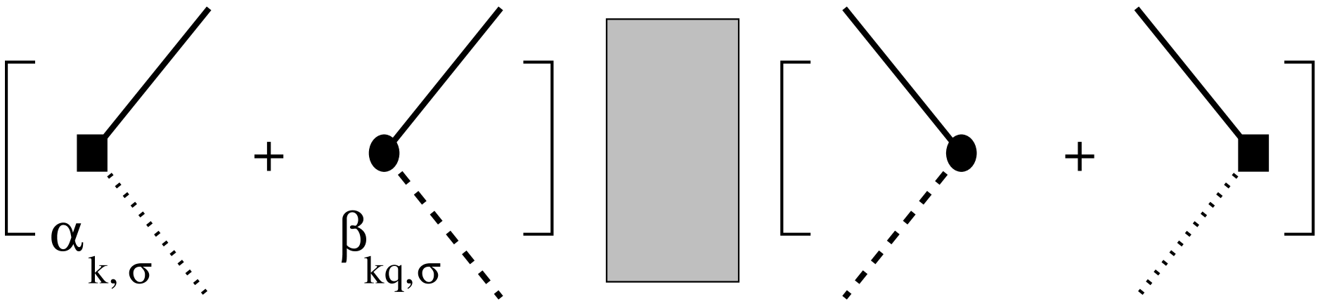
FIG. 3.: Structure of the physical Green’s function $G_{\sigma}^{c}(k,\omega)$. Solid, dashed, and dotted lines refer to pseudo-fermion, triplet, and singlet Green’s functions. Dashed box denotes reducible two particle vertex. In LHP approximation dotted lines collapse to unity.

FIG. 4.: LHP+RPA approximation to the physical Green’s function $G_{\sigma}^{c}(k,\omega)$.

For a finite albeit small density of triplet-pairs in the ground state, i.e. $0<v_{q}\ll 1$, we proceed by a perturbative evaluation of the two-particle propagator of fig. 3 using the RPA as shown in fig. 4. A comparable analysis of the effects of ground-state quantum fluctuations on the single-hole spectrum has been carried out in an AFM spin-background for the square-lattice $t$-$J$-model [59]. Within the RPA the physical Green’s function is given by

$$G_{\sigma}^{c}(k,w)=$$ (59)

$$\alpha_{k,\sigma}G_{\sigma}(k,w)\alpha_{k,\sigma}+\sum_{q}\beta_{kq,\sigma}G_{\sigma}(k-q,\omega-\omega_{q})\beta_{kq,\sigma}$$

$$+\pmatrix{\alpha_{k,\sigma}G_{\sigma}(k,w)&\sqrt{\frac{3}{N}}\sum_{q}\beta_{kq,\sigma}G_{\sigma}(k-q,\omega-\omega_{q})M^{\dagger}_{kq}}$$

$$\times\pmatrix{1&-\frac{3}{N}M_{kq}G_{\sigma}(k-q,\omega-\omega_{q})M^{\dagger}_{kq}\cr-G_{\sigma}(k,\omega)&1}^{-1}$$

$$\times\pmatrix{\sqrt{\frac{3}{N}}\sum_{q}M_{kq}G_{\sigma}(k-q,\omega-\omega_{q})\beta_{kq,\sigma}\cr G_{\sigma}(k,\omega)\alpha_{k,\sigma}}$$

where the element-by-element multiplication of the matrix and vector entries in the matrix-product on the last three lines of this equation are 2$\times$2 matrices operations. To arrive at (59) the LHP dynamics of the bond-bosons has been used which implies a constant factor of unity only in case of the singlet propagator.

Concluding this section we note the sum rule

$$\int_{-\infty}^{\infty}d\omega A_{\sigma}^{c}(k,\omega)=\{\phi^{\phantom{\dagger}}_{k,\sigma},\phi^{\dagger}_{k,\sigma}\}=\frac{1}{2}\pmatrix{1&0\cr 0&1}$$ (60)

for the exact physical Green’s function with $A_{\sigma}^{c}(k,\omega)=-\frac{1}{\pi}\mbox{Im}\;G_{\sigma}^{c}(k,\omega)$ at half-filling which differs from that for free fermions since the $\hat{c}_{i,n,\sigma}^{(\dagger)}$ are Hubbard operators. Integrating (60) we find that the combined LHP and RPA approach is consistent with this sum-rule yielding

$$-\frac{1}{\pi}\int_{-\infty}^{\infty}\mbox{Im}G^{c}_{\sigma}(k,\omega) =\alpha_{k,\sigma}^{2}+\sum_{q}\beta_{kq,\sigma}^{2}$$ (62)

$$=\frac{1}{2}\pmatrix{1&0\cr 0&1}(s^{2}+\frac{3}{N}\sum_{q}v_{q}^{2})$$

where the term in the last bracket is one due to (36).

VI Dimerized chain spectra

In the remaining sections of this work we will detail various results of the numerical solution of the SCBA and RPA equations. We begin with the dimerized-chain limit of the $t_{1,2,3}$-$J_{1,2,3}$-model, i.e. with $J_{3}=t_{3}=0$. In view of the non-zero dimerization it seems convenient to visualize the lattice geometry as that of a linear chain with a unit cell containing two electrons and a lattice constant $2a$, set equal to unity, where $a$ is the inter-site distance. In contrast to this, existing ED studies frequently employ a different representation in which each unit cell contains a single site only. This representation can be obtained by introducing the fermion operators

$$d_{\frac{k}{2},\sigma}=\frac{1}{\sqrt{2}}\left({\hat{c}}_{1,k,\sigma}+e^{-i\frac{k}{2}}{\hat{c}}_{2,k,\sigma}\right),$$ (63)

which we term $d$-electrons hereafter. The $d$-Green’s-function $G_{\sigma}^{d}(k,\omega)$ reads

$$G_{\sigma}^{d}(k,\omega) = \frac{1}{2}[(G_{\sigma}^{c}(k,\omega))_{11}+(G_{\sigma}^{c}(k,\omega))_{22}$$ (64)

$$+ e^{-i\frac{k}{2}}(G_{\sigma}^{c}(k,\omega))_{12}+e^{i\frac{k}{2}}(G_{\sigma}^{c}(k,\omega))_{21}],$$ (65)

with $A^{d}_{\sigma}(k,\omega)=-\frac{1}{\pi}\mbox{Im}\;G_{\sigma}^{d}(k,\omega)$ beeing the corresponding spectral function.

Selfconsistent solutions for the SCBA can be obtained quite easily by numerical iteration on fairly large lattices and for small, but finite imaginary broadening $\eta\ll 1$. Convergence of the iteration is achieved within a few, typically 3-20, cycles depending on the size of the spin gap. Moreover, finite size scaling analysis can be used to determine an approximate system size at which further increase in the number of lattice sites leads to no additional change in the pseudo-fermion Green’s function at fixed $\eta$, i.e. the thermodynamic limit. Inserting SCBA Green’s-functions from this limit into the RPA (59) we obtain typical spectra as displayed in fig. 5. The number of sites is $512=2\times N$ where $N$ is the number of dimers. The dimerization of the hopping integrals and the exchange couplings have been chosen independently with $t_{1}=t_{2}$ and $\delta$ such as to result in a spin gap of $\Delta/t_{1}=0.2J_{0}/t_{1}$. Since $J_{{}^{1}_{2}}=J_{0}(1\pm\delta)$ one finds $\Delta/t_{1}=[2(\delta^{2}+\delta)]^{1/2}J_{0}/t_{1}$. Figure 5a) (b)) refers to $J_{0}/t_{1}=1(0.5)$ and $\Delta/t_{1}=0.2(0.1)$. All spectra are particle-hole inverted, i.e. $\omega\rightarrow-\omega$, such as to place the first electron-removal state at the lowest binding-energy.

FIG. 5.: Spectral function of the dimerized chain for various values of momentum $k=0$ to $\pi$ and $t_{1}=t_{2}$, $N=256$, and $\eta=0.05$. (a) $J_{0}/t_{1}=1$, $\Delta/t_{1}=0.2$ and (b) $J_{0}/t_{1}=0.5$, $\Delta/t_{1}=0.1$.

FIG. 6.: Spectral function of the dimerized chain for various values of momentum $k=0$ to $\pi$ and $t_{1}=t_{2}=J_{0}$, $N=256$, and $\eta=0.05$. (a) $\Delta/t_{1}=0.05$ and (b) $\Delta/t_{1}=0.7$.

The figure displays two dominant dispersive regions which are related to the first three terms in Hamiltonian (35). These terms allow for coherent hole-motion without triplet excitations of the spin-background and lead to two tight-binding-type bands which are accounted for by $H_{0}$ in Hamiltonian (40). These tight-binding states are renormalized and broadened upon coupling to multi triplet-excitations via the SCBA. In particular the states of high binding-energy are broadened quite strongly. Comparing fig. 5a) vs. b) it is obvious that the amount of the spectral redistribution depends on the relative size of $J_{0}/t_{1}$, where decreasing $J_{0}/t_{1}$ implies a larger incoherent part of the spectrum. Additionally the dispersion flattens as $J_{0}/t_{1}$ decreases.

Finite-size analysis of the two sharp structures at the high-energy edge of the spectrum in figure 5a) (b)) reveals that for any finite spin-gap these structures refer to poles of the Green’s function on the real axis which remain separated by a gap from the continuum of multi-magnon shake-offs. The spectral weight of these poles remains finite in the thermodynamic limit. Therefore, the first electron removal state is of a quasi-particle type. The first of these two poles, i.e. at higher binding-energy, can be traced back to a quasi-particle excitation in the pseudo-fermion SCBA-spectrum which is shadowed in the physical fermion Green’s function. The second pole at lowest binding energy, i.e. the first electron removal state, arises from a zero of the determinant of the RPA-matrix propagator in (59). This can be interpreted in terms of a bound state between the aforementioned pseudo-fermion quasi-particle and the ground-state quantum fluctuations of the spin-system.

Figure 6 refers to the dependence of the spectra on the spin-gap displaying two additional values of $\delta$ different from that used in fig. 5. We find that the gap between the first electron-removal state and the second pole increases upon increasing the spin gap. Moreover the dispersion decreases for smaller values of $\delta$. For $\Delta/t_{1}=0.05J_{0}/t_{1}$ and $J_{0}=t_{1}$, fig. 5a), an intense low energy band arises. The dispersion of the two dominant spectral regions at $\delta\ll 1$ are reminiscent of similar findings for the infinite-$U$ Hubbard-chain at half filling [60].

Figure 7 shows the weight, i.e. the $Z$-factor, of the quasi-particle pole at wave vector $k=\pi/2$ as a function of various parameters, $\delta$, $J_{0}/t_{1}$, and $J_{3}/t_{1}$. The $Z$-factor has been determined by fitting a Lorentzian to the quasi-particle peak. The renormalization effects are quite strong for those parameters we have considered as $Z$ is reduced substantially from the non interacting value of one half (60). This figure demonstrates that a finite spin-gap stabilizes the quasi-particle excitations, while approaching the Heisenberg point, i.e. $\delta=0$, $J_{3}=0$, as in fig. 7a) suppresses the $Z$-factor due to the decrease in energy of available triplet excitations. In fig. 7b) the dimerization is kept at a constant value to result in $\Delta/t_{1}=0.2J_{0}/t_{1}$ with only $J_{0}/t_{1}$ varying. This leads to almost no change in the $Z$-factor. Increasing frustration, as in fig. 7c) increases both, the average absolute value of the vertex-function $M_{kq}$ of (41) and the spin-gap $\Delta$. These effects compete leading to only a slight increase of the $Z$-factor as a function of $J_{3}$. Here $\delta$ is still kept at the constant value of fig. 7b). While the single-hole case does not resemble a finite hole concentration it is tempting to relate the finite $Z$-factor in the presence of a spin-gap to a Luther-Emery-liquid [34] scenario in contrast to the Luttinger-liquid [35] at vanishing spin-gap.

FIG. 7.: Quasiparticle weight $Z(k=\pi/2)$ as a function (a) of $\Delta/t_{1}$ for $J_{0}=t_{1}$, $J_{3}=0$, (b) of $J_{0}/t_{1}$ for $\Delta/t_{1}=0.2J_{0}/t_{1}$, i.e. $\delta=const.$, $J_{3}=0$, and (c) of $J_{3}/t_{1}$ for $\delta$ as in (b), $J_{0}=t_{1}$. $N=256$, $t_{1}=t_{2}$.

Next we turn to a comparison of our diagrammatic approach with results obtained from exact diagonalization (ED) of finite chains. To this end, we contrast a single-hole spectrum for $\delta=0.048$ and $t_{1}=t_{2}=J_{0}$ reproduced from the work of Augier and collaborators [31] in fig. 8a) against a physical fermion Green’s function obtained via (59) using an identical number of sites in fig. 8b). The agreement, albeit qualitative, is rather satisfying. In 8b) the thin dashed line refers to the pseudo-fermion spectrum. Obviously the similarity of this function to the ED result is less convincing thereby demonstrating the relevance of ground-state quantum fluctuations. The difference between the pseudo- and the physical-fermion spectrum is particularly evident in the incoherent part at wave vectors larger than $\pi/2$.

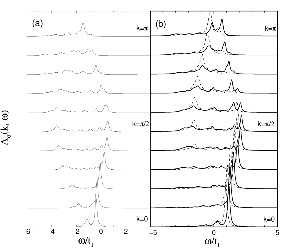
FIG. 8.: Comparison of spectra for a dimerized $20$-site chain for various values of momentum $k=0$ to $\pi$ and $t_{1}=t_{2}=J_{0}$, $\delta=0.048$. (a) ED data, reproduced from ref.³¹ (b) solid line SCBA+RPA spectrum $A^{d}_{\sigma}(k,\omega)$, dashed line SCBA-only spectrum $A^{a}_{\sigma}(k,\omega)$. $\eta=0.05$. (a) and (b) are shifted relative to each other due to differing zeros of energy.

Closing this section we comment on the so-called dimerized $t$-model limit, i.e. $t_{1}=t_{2}$, $J_{1}\gg J_{2}$ with $J_{1}\rightarrow 0$, and $t_{3}=J_{3}=0$. In this case the ground state of the spin system is a perfect dimer product-state while the only energy scale of the system is the hopping amplitude $t=t_{1}$. The local density of states $\rho(\omega)$ for a single hole in one dimension is known to be $\rho(\omega)=1/\sqrt{\omega^{2}-4t^{2}}$ which is independent of the particular spin-background [57]. Calculating $\rho_{d(a)}(\omega)=\frac{1}{2N}\sum_{k}A^{d(a)}_{\sigma}(k,\omega)$ using the representation (63) and (65) we obtain the result shown in fig 9. The SCBA+RPA approach shows some deviation from the exact result regarding the low-frequency regime and the overall band-width. The latter effect is reminiscent of similar findings from analysis of the 2D AFM $t$-model[54]. The pure SCBA pseudo-fermion spectrum shows little resemblance with the exact result.

FIG. 9.: $t$-model DOS for $N=256$ and $t_{1}=t_{2}$. Solid, long dashed, and short dashed line refer to the SCBA+RPA, i.e. $\rho_{d}(\omega)$, SCBA-only, i.e. $\rho_{a}(\omega)$, and Brinkman-Rice result⁵⁷.

VII Spin-ladder spectra

In this section we turn to the case of $J_{2}=t_{2}=0$ which describes a two-leg spin ladder. In contrast to the definition (63) of the fermions to account for the 1D representation, the unit cell remains identical to that of the lattice topology of fig. 1. The pseudo-fermion operators on a rung can be labeled according to their (anti)bonding symmetry and the reciprocal space is quasi two-dimensional with a wave vector ${\bf k}=(k,k_{y})$ where $k_{y}=(\pi)0$ which refers to the (anti)bonding state

$$b_{k,k_{y},\sigma}^{\dagger}=\frac{1}{\sqrt{2}}\left(a_{2,k,\sigma}^{\dagger}+e^{ik_{y}}a_{1,k,\sigma}^{\dagger}\right).$$ (66)

Expressing $G_{\sigma}^{c}(k,\omega)$ in terms of $b_{k,k_{y},\sigma}$ renders the Green’s function diagonal because the Hamiltonian conserves parity and the operators (66) exhibit a different signature with respect to reflections at a plane perpendicular to the rungs [61]. The pseudo and physical fermion spectral functions are labeled accordingly, i.e. $A^{a}_{0(\pi),\sigma}(k,\omega)$ and $A^{c}_{0(\pi),\sigma}(k,\omega)$, where the subscript $0(\pi)$ refers to the (anti)bonding symmetry.

Conservation of parity leads to an important constraint regarding the pseudo-fermion self-energy. Since the spin-triplet has odd parity, scattering of a pseudo-fermion off a triplet can occur only via a transition between the bonding and the antibonding fermionic states which have different parity. This implies a certain ’robustness’ of the bare pseudo-fermion bands of $H_{0}$ of (40) against renormalization by $V$ because of the finite energy gap $2t_{1}$ between the bare bands given by $\epsilon_{\pi(0)}(k)=(-)t_{1}+t_{3}\cos(k)$. Therefore, perturbative analysis of the single-hole dynamics on a ladder using methods complementary[50, 62] as well as related[32, 58] to that of this work have led to rather good agreement with numerical studies of finite system.

FIG. 10.: Spectral function $A^{c}_{0(\pi),\sigma}$ of the bonding ($0$) and antibonding $(\pi)$ bands of the two-leg ladder for various values of momentum $k=0$ to $\pi$. $N=256$, $\eta=0.1$. (a) $t_{1}=t_{3}$, $J_{1}/t_{1}=5$, $J_{3}/t_{1}=0.5$. (b) $t_{1}=t_{3}$, $J_{1}/t_{1}=1$, $J_{3}/t_{1}=0.1$.

In fig. 10a) the (anti)bonding spectra are shown for a case of strong intra-rung exchange $J_{1}/t_{1}=5$, $J_{3}/t_{1}=0.5$. The number of rungs is set to $N=256$ for which finite-size effects are negligible. The ground-state in this case is close to a pure singlet product-state with almost no quantum fluctuations. The spin-gap is relatively large, i.e. $\Delta/t_{1}\approx 4.5$. The spectrum clearly displays the remnants of the (anti)bonding bare bands and the intensity of the incoherent contributions to the spectrum are weak. Next, fig. 10b), with $J_{1}/t_{1}=1$, $J_{3}/t_{1}=0.1$, refers a smaller gap which accounts for the extra incoherence of the spectrum and the less correspondence between the bare and the renormalized bands. Moreover the high energy parts of the two bands intersect.

Unfortunately, at the isotropic point, i.e. $J_{1}=J_{3}$, the LHP approximation breaks down, with the spin-gap closing for $J_{3}\geq J_{1}/2$. Yet, from series expansion [43, 44, 63, 64] and DMRG [65] it is known, that $\Delta/J\approx 0.5$ in that case. To account for this deficiency of the LHP we keep the isotropic set of parameters in all of (40-41) however we adjust $J_{3}$ in (13-17) such as to result in $\Delta/J_{1}=0.5$. We believe that this modification provides an approximate description of the renormalization of $\omega_{k}$ which occurs beyond the LHP approach.

FIG. 11.: Spectral function $A^{c}_{0(\pi),\sigma}$ of the bonding ($0$) and antibonding $(\pi)$ bands of the two-leg ladder for various values of momentum $k=0$ to $\pi$ at the isotropic point $t_{1}=t_{3}=J_{1}=J_{3}$. $N=256$, $\eta=0.1$. (a) complete spectrum (b) details at low binding-energy.

Fig. 11a) and b) display the case of isotropic exchange and hopping, i.e. $t_{1}=t_{3}=J_{1}=J_{3}$. Here the renormalization of the free particle bands is very strong. The bonding band at highest frequency, is very flat. In the antibonding band the intensity at highest energy is a composite excitation of states from the bonding band and a single triplet. Its relatively large intensity is a result of parity conservation, which inhibits intraband scattering. In addition a lower energy feature, reminiscent of the free antibonding band, can be observed at in the vicinity of $k=\pi$. Fig. 11b) shows a stretched frequency window with the two bands of lowest binding energy. Interestingly, the maximum of the dispersion is found off the momenta $k=0$ or $\pi$. This is consistent with ED studies [28] and series expansions [66].

Analogous to the case of the linear chain we contrast our diagrammatic calculation against ED analysis. In fig. 12a) a spectrum reproduced from the work of Haas and collaborators [30] is compared to a physical-fermion spectrum obtained from the SCBA+RPA approach. The latter spectrum is shown in fig. 12b). It compares well with the ED result. Finally the dashed line in 12b) displays the SCBA, i.e. pseudo-fermion spectrum. The latter spectrum lacks the large intensity in the high energy region of the antibonding band and the displacement of the maximum of the dispersion at low binding energy mentioned in the previous paragraph. This demonstrates that an inclusion of ground-state quantum-fluctuations is mandatory for a proper description of the single-hole dynamics in this regime of parameters.

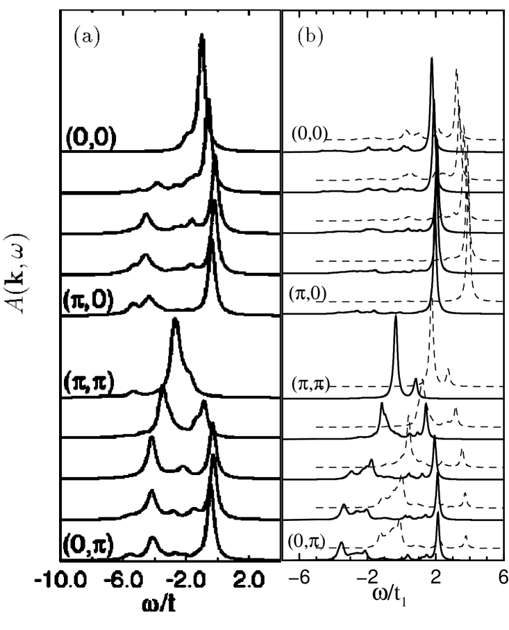
FIG. 12.: Comparison of spectra for an $N=8$-rung two-leg spin-ladder for various values of momentum $k=0$ to $\pi$. $t_{1}=t_{3}=J_{1}=J_{3}$, and $\eta=0.1$. (a) ED data, reproduced from ref.³⁰ (b) solid line SCBA+RPA spectrum $A^{c}_{\sigma}({\bf k},\omega)$, dashed line SCBA-only spectrum $A^{a}_{\sigma}({\bf k},\omega)$. For better visibility the SCBA-only spectra have been shifted by $\Delta\omega/t=2$ along the $x$, an arbitrary amount along the $y$ axis.

VIII Conclusion

In conclusion we have investigated the single-hole excitations at half filling in dimerized and frustrated spin-chains and ladders in the spin-dimer phase. Based on an analytic approach we have provided a physically intuitive picture of the single-hole dynamics as resulting from a combination of the dimerization of the spin background and the scattering of the holes by massive triplet-modes of the spin system. Due to the spin-gap we find, that the single-hole excitations are quasi-particle like though strongly renormalized. The impact of ground state quantum fluctuations of the dimer state on the hole-spectrum has been elucidated. Our results compares well with numerical diagonalization of finite systems, both for chains and ladders. We hope that our work will promote future experimental studies to obtain angular resolved photoemission spectra on the novel chain-and ladder-type transition-metal oxides in an energy window comparable to the magnetic exchange coupling.

It is a pleasure to acknowledge helpful discussions with G. Baskaran, M. Brunner, R. Eder, and O. Sushkov. This research was supported in part by the Deutsche Forschungsgemeinschaft under Grant No. BR 1084/1-1.

REFERENCES

- [1] A. W. Garrett, S. E. Nagler, D. A. Tennant, B. C. Sales, and T. Barnes, Phys. Rev. Lett. 79, 745 (1997).
- [2] B. Lake, D. A. Tennant, R. A. Cowley, J. D. Axe, and C. K. Chen, J. Phys.: Condens. Matter 8, 8613 (1996).
- [3] J. C. Bonner, S. A. Friedberg, H. Kobayashi, D. L. Meier, and H. W. J. Blöte, Phys. Rev. B 27, 248 (1983).
- [4] M. Hase, I. Terasaki, and K. Uchinokura, Phys. Rev. Lett. 70, 3651 (1993).
- [5] M. Isobe and Y. Ueda, J. Phys. Soc. Jpn. 65, 1178 (1996).
- [6] L.N. Bulaevskii, A. I. Buzdin, and D.I. Khomskii, Sol. State Commun. 27, 5 (1978).
- [7] G. Castilla, S. Chakravarty and V.J. Emery, Phys. Rev. Lett. 75, 1823 (1995).
- [8] J. Riera and A. Dobry, Phys. Rev. B 51, 16098 (1995).
- [9] H. Smolinski, C. Gros, W. Weber, U. Peuchert, G. Roth, M. Weiden, and C. Geibel, Phys. Rev. Lett. 80, 5164 (1998).
- [10] Z. Hiroi, M. Azuma, M. Takano and Y. Bando, J. Solid State Chem. 95, 230 (1991); M. Azuma, Z. Hiroi, M. Takano, K. Ishida and Y. Kitaoka, Phys. Rev. Lett. 73, 3463 (1994).
- [11] H. Iwase, M. Isobe, Y. Ueda and H. Yasuoka, J. Phys. Soc. Jpn. 65 2397 (1996).
- [12] G. Chaboussant, P. A. Crowell, L. P. Lévy, O. Piovesana, A. Madouri, and D. Mailly, Phys. Rev. B 55, 3046 (1997).
- [13] H. Kageyama, K. Yoshimura, R. Stern, N. V. Mushnikov, K. Onizuka, M. Kato, K. Kosuge, C. P. Slichter, T. Goto, and Y. Ueda, Phys. Rev. Lett. 82, 3168 (1999).
- [14] S. Miyahara and K. Ueda, Phys. Rev. Lett. 82, 3701 (1999).
- [15] B. S. Shastry and B. Sutherland, Phys. Rev. Lett. 47, 964 (1981); B. S. Shastry and B. Sutherland, Physica 108B, 1069 (1981).
- [16] C. K. Majumdar and D. K. Ghosh, J. Math. Phys. 10, 1388 and 1399 (1969); C. K. Majumdar, J. Phys.: Condens. Matter 3, 911 (1970).
- [17] N. Motoyama, H. Eisaki and S. Uchida, Phys. Rev. Lett. 76, 3212 (1996).
- [18] C.L. Teske and H. Müller-Buschbaum, Z. Anorg. Allg. Chem. 371, 325 (1969); C.L. Teske and H. Müller-Buschbaum, Z. Anorg. Allg. Chem. 379, 234 (1970).
- [19] M. Cross and D. S. Fisher, Phys. Rev. 19, 402 (1979); M. C. Cross, ibid 20, 4606 (1979).
- [20] K. Okamoto and K. Nomura, Phys. Lett. A 169, 433 (1992).
- [21] R. Chitra, S. Pati, H. R. Krishnamurthy, D. Sen, S. Ramasesha, Phys. Rev. B 52, 6581 (1995).
- [22] For reviews see [23] and: E. Dagotto and T. M. Rice, Science 271, 618 (1996); M. Takano, Physica C 263, 468 (1996); S. Maekawa, Science 273, 1515 (1996); T. M. Rice, Z. Phys. B 103, 165 (1997); H. Tsunetsugu, Physica B 237–238, 108 (1997).
- [23] E. Dagotto, cond-mat/9908250; Rep. Prog. Phys. 62, 1525 (1999).
- [24] M. Uehara, T. Nagata, J. Akimitsu, H. Takahashi, N. Mori, and K. Kinoshita, J. Phys. Soc. Jpn. 65, 2764 (1996).
- [25] E.M. McCarron, M.A. Subramanian, J.C. Calabrese, und R.L. Harlow, Mater. Res. Bul. 23, 1355 (1988)
- [26] H. Tsunetsugu, M. Troyer, and T. M. Rice, Phys. Rev. B 49, 16078 (1994).
- [27] H. Tsunetsugu, M. Troyer, and T. M. Rice, Phys. Rev. B 51, 16456 (1995).
- [28] M. Troyer, H. Tsunetsugu, and T. M. Rice, Phys. Rev. B 53, 251 (1996).
- [29] S.Haas and E. Dagotto, Phys. Rev. B52, R14396 (1995).
- [30] S. Haas and E. Dagotto, Phys. Rev. B 54, R3718 (1996).
- [31] D. Augier, D. Poilblanc, S. Haas, A. Delia and E. Dagotto, Phys. Rev. B 56, R5732 (1997).
- [32] R. Eder, Phys. Rev. B 57, 12832 (1998).
- [33] G. Martins, C. Gazza, and E. Dagotto, Phys. Rev. B 59, 13596 (1999).
- [34] A. Luther and V.J. Emery, Phys. Rev. Lett. 33, 589 (1974); V.J. Emery, in Highly Conducting One-Dimensional Solids, edited by J.T. Devreese et al. (Plenum, New York, 1979).
- [35] F.D.M. Haldane, Phys. Rev. Lett. 45, 1358 (1980); J. Phys. C 14, 2585 (1981).
- [36] S. Sachdev and R. N. Bhatt, Phys. Rev. B 41, 9323 (1990).
- [37] A. V. Chubukov, Pis’ma Zh. Eksp. Teor. Fiz. 49, 108 (1989); [JETP Lett. 49, 129 (1989)].
- [38] A. V. Chubukov and Th. Jolicoeur, Phys. Rev. B 44, 12050 (1991).
- [39] O. A. Starykh, M. E. Zhitomirsky, D. I. Khomskii, R. R. P. Singh, and K. Ueda, Phys. Rev. Lett. 77, 2558 (1996).
- [40] W. Brenig, Phys. Rev. B 56, 14441 (1997).
- [41] A. Brooks Harris, Phys. Rev. B 7, 3166 (1973).
- [42] G. Uhrig, Phys. Rev. Lett. 79, 163 (1997).
- [43] M. Reigrotzki, H. Tsunetsugu, and T. M. Rice, J. Phys.: Condens. Matter 6, 9235 (1994).
- [44] T. Barnes, E. Dagotto, J. Riera, and E. S. Swanson, Phys. Rev. B, 3196 (1993).
- [45] C. Gros and R. Valentí, Phys. Rev. Lett. 82, 976 (1999).
- [46] O.P. Sushkov and V.N. Kotov Phys. Rev. Lett. 81, 1941 (1998)
- [47] V. N. Kotov, O. P. Sushkov, and R. Eder, Phys. Rev. B, 6266 (1999).
- [48] C. Jurecka and W. Brenig Phys. Rev. B 61, 14307 (2000).
- [49] V. N. Kotov, O. P. Sushkov, Z. Weihong, and J. Oitmaa, Phys. Rev. Lett. 80, 5790 (1998).
- [50] O. P. Sushkov, Phys. Rev. B 60, 3289 (1999).
- [51] M. Vojta and K. Becker, Phys. Rev. B 60, 15201 (1999).
- [52] C. Jurecka, unpublished
- [53] S. Schmitt-Rink and C.M. Varma, Phys. Rev. Lett. 60, 2793 (1988).
- [54] C. L. Kane, P. A. Lee, N. Read, Phys. Rev. B 39, 6880 (1989).
- [55] G. Martinez, P. Horsch, Phys. Rev. B 44, 317 (1991).
- [56] Z. Liu, E. Manousakis, Phys. Rev. B 45, 2425 (1992).
- [57] W. F. Brinkman and T. M. Rice, Phys. Rev. B 2, 1324 (1970).
- [58] In [32] a version of eqn. (50) has been considered for the spin ladder with the term ’’ in the argument of the selfenergy lacking. We are unable to reproduce this form of the SCBA. In turn, the SCBA-spectra found in [32] differ considerably from ours.
- [59] O.P. Sushkov, G.A. Sawatzky, R. Eder and H. Eskes, Phys. Rev. B 56, 11769 (1997).
- [60] S. Sorella and A. Parola, J. Phys.: Condensed Matter 4, 3589 (1992)
- [61] S. Gopalan, T. M. Rice, M. Sigrist, Phys. Rev. B 49, 8901 (1994).
- [62] H. Endres, R. M. Noack, W. Hanke, D. Poilblanc and D. J. Scalapino, Phys. Rev. B 53, 5530 (1996).
- [63] J. Oitmaa, R. P. Singh, Z. Weihong, Phys. Rev. B 54, 1009 (1996).
- [64] J. Piekarewicz, J. R. Shepard, Phys. Rev. B 58, 9326 (1998).
- [65] S. R. White, R. Noack, D. J. Scalapino, Phys. Rev. Lett. 73, 886 (1994).
- [66] J. Oitmaa, C. J. Hamer, Z. Weihong, Phys. Rev. B 60, 16364 (1999).