Microscopic theory for quantum mirages in quantum corrals

Abstract

Scanning tunneling microscopy permits to image the Kondo resonance of a single magnetic atom adsorbed on a metallic surface. When the magnetic impurity is placed at the focus of an elliptical quantum corral, a Kondo resonance has been recently observed both on top of the impurity and on top of the focus where no magnetic impurity is present. This projection of the Kondo resonance to a remote point on the surface is referred to as quantum mirage. We present a quantum mechanical theory for the quantum mirage inside an ideal quantum corral and predict that the mirage will occur in corrals with shapes other than elliptical.

I Introduction

Scanning Tunneling Microscopy (STM) allows the manipulation of single atoms on top of a surface [1] as well as the construction of quantum structures of arbitrary shape. Additionally, the differential conductance, $G(V)\equiv dI/dV$, is proportional to the local density of states (LDOS) of the surface spot below the tip [2]. Hence, STM can be used to modify and to measure the LDOS.

A STM was used by Crommie et al. to build a quantum corral, i.e., a 71 $\AA$ radius circle made with 48 atoms of iron on top of a surface of copper [3]. The free motion of the electrons along the surface changed in the presence of the Fe atoms so that quasi-bound states appeared inside the corral. The measured LDOS was quite similar to that of a gas of noninteracting electrons inside a circular confining potential.

More recently, STM has permitted to study the problem of a single magnetic impurity embedded in the two dimensional electron gas formed on a metallic surface [4, 5]. This is the famous Kondo problem. Below the Kondo temperature, $T_{K}$, a many electron singlet state forms so that the spin of the magnetic impurity is screened by the conduction electrons. As a consequence, the impurity density of states develops a resonance at the Fermi energy (the Abrikosov-Suhl resonance [6, 7]). When the STM tip is placed on top of the magnetic impurity, $G(V)$ displays a narrow dip around the Fermi level [4, 5]. The dip (instead of the resonance) is due to a Fano type interference between the direct tunneling from the tip to the surface and the additional chanels that appear due to the presence of the impurity [4, 5, 8, 9]. The depth of the dip decreases gradually as the lateral distance between the tip and the impurity is increased. This permits to image the magnetic atom. The dip vanishes when lateral tip-magnetic impurity distance is bigger than $10\AA$, which is twice $k^{-1}_{F}$, the inverse of the Fermi vector.

This situation is dramatically changed when the magnetic impurity is placed at the focus of an elliptical corral of size smaller than 150 $\AA$ [10], built on the Cu(111) surface. In this configuration, the Kondo dip is observed not only on the focus where the magnetic impurity is located but also on the empty focus, which can be as far as 110 $\AA$ away from the impurity. Remarkably, the phantom dip is not observed if either the tip or the impurity are not at the foci. The phenomenon of the phantom dip is referred to as the quantum mirage [10]. In this paper we provide a quantum mechanical theory for this phenomenon. In particular we want to address the issue of under which conditions the quantum mirage can be observed and whether an elliptical corral is necessary to obtain the mirage. We show that the elliptical geometry is convenient but not necessary and we show that there is no need to invoke semiclassical arguments to explain the mirage.

The structure of this paper is the following: In section II we review the theoretical framework adequate to study the quantum mirage. First, we present the Hamiltonian of a surface with both a magnetic impurity and a quantum corral. Then we give a formal expression for the relation between $G(V)$ and the surface LDOS. Our original contribution starts in section III, where we give a qualitative explanation for the quantum mirage. In section IV we present quantitative results for elliptical quantum corrals and in section V we discuss our results as well as the limitations of our theory.

II Theoretical Framework

A The Hamiltonian of the surface

The Hamiltonian of the surface is an extension of the well known Anderson model[11] to the case in which the electrons feel the potential produced by the atoms creating the corral:

$$H_{\rm surf}=\sum_{n,\sigma}\epsilon_{n}c_{n,\sigma}^{\dagger}c_{n,\sigma}+\epsilon_{d}\sum_{\sigma}{d_{\sigma}^{\dagger}}d_{\sigma}$$ (1)

$$+Ud^{\dagger}_{\uparrow}d_{\uparrow}d^{\dagger}_{\downarrow}d_{\downarrow}+V_{h}\sum_{n,\sigma}\psi^{*}_{n}(\vec{R}_{I})c_{n,\sigma}^{\dagger}d_{\sigma}+h.c..$$ (2)

$\epsilon_{n}$ and $\psi_{n}(\vec{R})$ are the eigenvalues and eigenfunctions of the surface corral Hamiltonian. $c_{n,\sigma}^{\dagger}$ and $d_{\sigma}^{\dagger}$ create an electron in the state $n$ of the corral, and in the magnetic impurity, respectively. In this work we only consider the states from the metallic surface band, which seem to give the main contribution to the LDOS measured by the STM [2, 3, 10]. The first term in (2) describes the Fermi sea formed by filling these states. The second term in (2) is the impurity single particle energy. The third term is the on-site repulsion felt whenever two electrons are at the impurity site. The last term describes the hopping between the surface and the impurity states. In the Anderson model, this coupling is localized at the impurity site, $\vec{R}_{I}$. From the formal point of view, the presence of the corral is accounted for by replacing the plane waves, which diagonalize the free surface electron Hamiltonian, by the corral states. Throughout the paper we neglect the magnetic moment of the corral atoms. This is justified because the mirage appears also when the corral atoms are non-magnetic [10].

It must also be noted that Hamiltonian (2) does not contain any scattering from the surface states to the bulk states, a process which could occur due to the presence of both the impurity and the corral atoms. These physical processes should be considered in order to have a more quantitative theory of this system, something beyond the scope of this paper.

B $G(V,\vec{R})$ vs. LDOS

We now review the link between the quantity measured in the experiments, $G(V,\vec{R})=dI/dV(\vec{R})$, the differential conductance measured when the tip is at position $\vec{R}$ on the surface, and the surface Green’s function, ${\cal G}_{S}(\vec{R},\epsilon^{+})$. The Hamiltonian of the whole system, tip and surface, can be written as the sum of three terms, $H=H_{\rm tip}+H_{\rm surf}+H_{\rm tun}$. The first is the Hamiltonian of the tip. The second, given in equation (2), corresponds to the Hamiltonian of the surface, including the corral and the magnetic impurity. The third is the tunneling (Bardeen) Hamiltonian, which describes processes in which an electron is transferred between the tip and the surface [9, 12]:

$$H_{\rm tun}=\sum_{\sigma}A^{\dagger}_{\sigma}\left(t_{c}\Psi_{\sigma}(\vec{R})+t_{d}d_{\sigma}\right)+h.c.,$$ (3)

where

$$\Psi^{\dagger}_{\sigma}(\vec{R})=\sum_{n}\psi^{*}_{n}(\vec{R})c^{\dagger}_{n,\sigma},$$ (4)

creates a surface electron in the spin state $\sigma$ at the position $\vec{R}$ of the surface and $A^{\dagger}_{\sigma}$ creates an electron in the tip. $t_{c}$ is the tunneling amplitude to the surface states and $t_{d}$ is the amplitude for tunneling directly to the magnetic impurity. $t_{d}$ has to be taken into account only when the tip is located very near the magnetic adatom ($\vec{R}\approx\vec{R}_{I}$). We assume the knowledge of the eigenstates of the tip and the surface Hamiltonians and treat the tunneling term as a perturbation. To lowest order in the tunneling Hamiltonian and low enough temperatures, linear response predicts [9, 13]:

$$\frac{dI}{dV}(\vec{R})\equiv G(V,\vec{R})=\frac{4e^{2}}{\pi\hbar}\rho_{T}\rho_{S}(\epsilon_{F}+eV,\vec{R}),$$ (5)

where $eV$ is the voltage drop and $\rho_{T}$ is the density of states of the tip (assumed to be energy independent in the vicinity of $\epsilon_{F}$). We follow the convention that positive $eV$ means electrons flowing towards the surface. Finally, the local density of states of the surface, $\rho_{S}$, is related to the retarded surface Green’s function through the relation:

$$\rho_{S}(\vec{R},\epsilon_{F}+eV)=-\frac{1}{\pi}Im\left[{\cal G}_{S}(\vec{R},\epsilon_{F}+eV)\right].$$ (6)

$\cal{G}_{S}$ is the retarded Green’s function corresponding to the operator $t_{c}\Psi_{\sigma}(\vec{R})+t_{d}d_{\sigma}$, and is given by [6, 9]:

$${\cal G}_{S}(\vec{R},\epsilon^{+})=t^{2}_{c}{\cal G}_{c}(\vec{R},\vec{R},\epsilon^{+})+{\cal G}_{d}(\epsilon^{+})\times$$ (7)

$$\left(t_{d}+t_{c}V_{h}{\cal G}_{c}(\vec{R},\vec{R}_{I},\epsilon^{+})\right)\left(t_{d}+t_{c}V_{h}{\cal G}_{c}(\vec{R}_{I},\vec{R},\epsilon^{+})\right),$$ (8)

where $\epsilon^{+}\equiv\epsilon+i\eta$. In the surface Green’s function (8), two different propagators appear. The first is the impurity free ($U=0$, $V_{h}=0$) surface Green’s function:

$${\cal G}_{c}(\vec{R}_{1},\vec{R}_{2},\epsilon^{+})=\sum_{n}\frac{\psi^{*}_{n}(\vec{R}_{1})\psi_{n}(\vec{R}_{2})}{\epsilon^{+}-\epsilon_{n}}.$$ (9)

The second is the Green’s function at the impurity site, whose evaluation is the difficult part of the many body problem [6]. For temperatures much lower than $T_{K}$, ${\cal G}_{d}$ can be approximated by the Green’s function of an effective resonant level with a broadening $T_{K}$:

$${\cal G}_{d}(\epsilon^{+})=\frac{Z_{K}}{\epsilon-\epsilon_{F}+ik_{B}T_{K}},$$ (10)

where $Z_{K}$ is chosen so that the impurity propagator fulfills the Friedel sum rule [6]:

$$Z_{K}\approx\frac{T_{K}}{\pi V_{h}^{2}\rho},$$ (11)

where $\rho=-\frac{1}{\pi}Im\left[{\cal{G}}_{c}(\vec{R}_{I},\vec{R}_{I},\epsilon_{F})\right]$ is the impurity free surface LDOS at the impurity site and at $\epsilon_{F}$. A necessary condition for the appearance of the Kondo resonance is that the conduction band is formed by a quasi-continuum of states, with energy spacing $\Delta<T_{K}$ [14]. In the case of the quantum corrals that we study below $\Delta>T_{K}$. However, the broadening, $\delta$, of these states, fulfills $\delta>T_{K}$, so that the density of states (in the absence of the magnetic impurity) is almost flat close to $\epsilon_{F}$ and we can use equation (10).

The surface Green’s function can be expressed now as:

$${\cal G}_{S}(\vec{R},\epsilon^{+})=t^{2}_{c}\left({\cal G}_{c}(\vec{R},\vec{R},\epsilon^{+})+\frac{T_{K}/\pi\rho}{\epsilon-\epsilon_{F}+ik_{B}T_{k}}\times\right.$$ (12)

$$\left.\left(\frac{t_{d}}{t_{c}V_{h}}+{\cal G}_{c}(\vec{R},\vec{R}_{I},\epsilon^{+})\right)\left(\frac{t_{d}}{t_{c}V_{h}}+{\cal G}_{c}(\vec{R}_{I},\vec{R},\epsilon^{+})\right)\right).$$ (13)

For the case $t_{d}=0$ (tip located far from the magnetic impurity) we can eliminate the parameter $V_{h}$ from our problem, due to the Friedel sum rule. When the tip is placed exactly at the magnetic impurity site ($\vec{R}=\vec{R}_{I}$), $t_{d}$ is no longer zero and we need to estimate the parameter $t_{d}/(t_{c}V_{h})$. To do that, we proceed as follows. In the absence of corral atoms, we can approximate the impurity free surface Green’s function by ${\cal{G}}_{c}(\vec{R}_{I},\vec{R}_{I},\epsilon^{+})\approx-i\rho_{0}$ and one obtains the well known Fano function for the differential conductance through the tip [5, 9]:

$$G(V,\vec{R}_{I})=\frac{4e^{2}}{\pi\hbar}\rho_{T}\rho_{0}t_{c}^{2}\frac{(q+\epsilon^{\prime})^{2}}{1+{\epsilon^{\prime}}^{2}},$$ (14)

where $\epsilon^{\prime}=(eV-\epsilon_{F})/T_{K}$, $\pi\rho_{0}q=t_{d}/(t_{c}V_{h})$ and $\rho_{0}$ is the LDOS at the Fermi Level for the surface states in the absence of quantum corral. $q$ is the Fano parameter which determines the shape of the $G(V,\vec{R}_{I})$ curves. It can can take values between 0 (symmetric dip) and $\infty$ (Breit-Wigner). We obtain $q$, and therefore $t_{d}/(t_{c}V_{h})$, by fitting the $G(V,\vec{R}_{I})$ curve to the Fano lineshape in the case of tunneling through the magnetic adatom in the absence of corral.

III The Quantum Mirage: Qualitative Explanation

In this section we give a qualitative explanation of the mirage, based on the general formalism of the previous section. We need to do several plausible hypothesis:

We suppose that the mirage is produced by quasi-bound states of the corral (an assumption that is consistent with the experiments [10]). Hence, we approximate the conduction Green’s function by:

$${\cal G}_{c}(\vec{R}_{1},\vec{R}_{2},\epsilon^{+})\approx\sum_{n}\frac{\psi^{*}_{n}(\vec{R}_{1})\psi_{n}(\vec{R}_{2})}{\epsilon-\epsilon_{n}+i\delta},$$ (15)

where $\delta$, the broadening of the quasi-bound corral states, is roughly 20 meV [15].

An additional approximation can be done if any of the two following statements holds:

• The level spacing between the energies of the quasi-bound states is much bigger than $\delta$.

• The level spacing is lower than $\delta$ but, due to the geometry of the quantum corral, only a few of the bound wavefunctions take a non-negligible value at the magnetic impurity site, $\vec{R}_{I}$. If the energy separation of these states is bigger than $\delta$, then only one of these states will transmit the quantum mirage, as it is evident from equation (15). This condition is fulfilled in the case of the elliptic corral, as we will show below.

In any of these two situations, whenever there is a quasi-bound state which simultaneously has an energy near $\epsilon_{F}$ and a non-negligible density at $\vec{R}_{I}$, we can replace equation (15) in (13) by:

$${\cal G}_{c}(\vec{R},\vec{R}_{I},\epsilon^{+})\approx\frac{\psi^{*}_{\epsilon_{F}}(\vec{R})\psi_{\epsilon_{F}}(\vec{R}_{I})}{\epsilon-\epsilon_{F}+i\delta}.$$ (16)

In next section we shall use the complete expression (15) for our calculations.

Our last approximation is to assume $t_{d}<<t_{c}$. A finite $t_{d}$ is considered in next section.

When we put together all these approximations, the change in $G(V,\vec{R})$ due to the presence of the impurity in $\vec{R}_{I}$ reads:

$$\delta G(V,\vec{R})\approx-\frac{4e^{2}V^{2}_{h}t^{2}_{c}}{\pi^{2}\hbar}\rho_{T}|\psi_{\epsilon_{F}}(\vec{R})|^{2}|\psi_{\epsilon_{F}}(\vec{R}_{I})|^{2}\times$$ (17)

$$Im\left(\frac{1}{(eV+i\delta)^{2}}\frac{1}{eV+ik_{B}T_{K}}\right).$$ (18)

For $eV<<\delta$ we can write:

$$\delta G(V,\vec{R})\propto-|\psi_{\epsilon_{F}}(\vec{R})|^{2}|\psi_{\epsilon_{F}}(\vec{R}_{I})|^{2}\frac{k_{B}T_{K}}{(eV)^{2}+(k_{B}T_{K})^{2}}.$$ (19)

Equation (19) is the most important result of this section. We want to highlight several points:

i) The spectral change in $G(V)$ is a dip of width $k_{B}T_{K}$ centered around $eV=0$, as observed in the experiments [4, 5, 10].

ii) According to equation (19), the dip is projected to any point $\vec{R}$ of the corral with an strength given by $|\psi_{\epsilon_{F}}(\vec{R})|^{2}|\psi_{\epsilon_{F}}(\vec{R}_{I})|^{2}$. Therefore, the projection is magnified when both the impurity and the tip are at points where the Fermi level corral wavefunction peaks. The projection disappears when either the impurity or the observation point, are located in a minimum. As we show in the next section, for the eccentricity of the experiment [10] the wavefunction of the elliptical corral at the Fermi level has its maxima close, but not at the foci. This result is in agreement with the experimental observation, but reduces the importance of the role played by the foci.

iii) The wavefunction at the Fermi level of any quantum corral has several maxima so that we predict that the mirage can be observed in other geometries. A possible candidate is the stadium corral shown in figure 3 of reference [16]. Therefore, an elliptical geometry is not needed to observe the mirage.

To conclude this section, we compare equation (19), valid for a confined geometry, with the case of an impurity in a translationally invariant surface. In both cases the surface Green’s function, ${\cal G}_{s}$, is the sum of two contributions, the impurity free contribution, ${\cal G}_{c}$, and the scattering contribution (see equation (8)). The first accounts for the paths in which the electron does not interact with the impurity and the second accounts for the paths in which the electron does indeed interact with the impurity. Hence, the local density of states in any point of the surface contains information about the impurity.

In the case of the free surface (without corral), a continuum of quantum states with different $\vec{k}$ carries that information so that destructive interference takes place at distances of the order of $2k_{F}^{-1}$, the inverse of the Fermi vector [6]. In contrast, when the electrons interact with the corral atoms, the information is carried, essentially, by a few quantum states, so that the destructive interference is less efficient. Equation (19) is derived assuming that a single quantum state is carrying the information so that there is no interference at all.

IV The mirage in the ellipse

In this section we study the mirage in an elliptical corral. Following the ideas of the previous section, we model the Green’s function of the surface states by that of the electrons confined in an hard wall elliptical corral. In order to compare with experiment [10], we consider the case in which the corral is built on a Cu(111) surface. We replace the real eigenvalues of the corral, $\epsilon_{n}$, by $\epsilon_{n}-i\delta$, in order to model the inelastic processes, such as scattering to the bulk states. It turns out that the problem of a quantum particle confined in an ellipse can be solved analytically . To do that, we write the Schrödinger equation in elliptical coordinates:

$$x = aeCos[\theta]Cosh[\eta]$$ (20)

$$y = aeSin[\theta]Sinh[\eta],$$ (21)

where $a$ and $e$ are the semimajor axis and eccentricity, respectively. The Helmholtz equation in this coordinate system is separable, so that the eigenstates of the problem can be written as:

$$\psi(\theta,\eta)=\Theta(\theta)\Lambda(\eta).$$ (22)

The Schrödinger equation is written as

$$\frac{d^{2}\Lambda(\eta)}{d\eta^{2}} - (\alpha-2kCosh[2\eta])\Lambda(\eta)=0$$ (23)

$$\frac{d^{2}\Theta(\theta)}{d\theta^{2}} + (\alpha-2kCos[2\theta])\Theta(\theta)=0$$ (24)

$$k = \frac{m^{*}(ea)^{2}\epsilon}{2\hbar^{2}},$$ (25)

where $\alpha$ is the separation constant, $\epsilon$ is the particle energy and $m^{*}$ is the electron effective mass which, in the Cu(111) surface band is $0.38$ $m_{e}$ [2, 3]. For a given $k$, only a discrete set of $\alpha_{r}(k)$ meet the requirement $\Theta(\theta)=\Theta(\theta+2pi)$. The elliptical hard wall condition reads $\Lambda(\eta_{0})=0$. It is clear that $\eta=\eta_{0}$ defines an ellipse of eccentricity $e=(Cosh[\eta_{0}])^{(-1)}$. For each $\alpha_{r}(k)$ there is a discrete number of $k_{n}$ compatible with the hard wall boundary condition. With all this in mind, we find 2 types of physically possible solutions for the particle inside the hard wall ellipse:

$$\psi_{n,c}(\theta,\eta) = ce_{r}(k^{c}_{n},\theta)Ce_{r}(k^{c}_{n},\eta)$$ (26)

$$\psi_{n,s}(\theta,\eta) = se_{r}(k^{s}_{n},\theta)Se_{r}(k^{s}_{n},\eta),$$ (27)

where $ce$, $se$, $Se$ and $Ce$ are the Mathieu functions [17] . Of course, we have $Se_{r}(k^{s}_{n},\eta_{0})=0$ and $Ce_{r}(k^{c}_{n},\eta_{0})=0$. These equations permit to find the spectrum. In figure 1 we plot a part of the spectrum of an ellipse with $e=0.5$ and $a=71.3\AA$.

In figure 2 we plot the LDOS at the focus in the absence of a magnetic impurity. It is clear that only a few states of figure 1 contribute significantly to the LDOS at the focus. The energy separation between these levels is much larger than $\delta=20meV$. There is one of these quasi-bound wavefunctions that has an energy of 447.5 meV, very near $\epsilon_{F}$ (which, for the Cu(111) surface band is 450 meV). We can thus explain the experimental observation of a quantum mirage in this quantum corral [10] using the results of section III.

FIG. 1.: Energy spectrum of an elliptical quantum corral with $e=0.5$ and semimajor axis, $a=71.3\AA$, on a Cu(111) surface.

FIG. 2.: LDOS at a focus of the elliptical quantum corral with $e=0.5$, $a=71.3\AA$ when no magnetic impurity is present.

In the left panel of figure 3 we show a contour plot of the wavefunction at the Fermi level for this ellipse. It must be stressed that the Fermi wavefunction maxima are located at a distance of 3.28 $\AA$ of the closest focus. The lattice constant of Cu(111) is 2.55 $\AA$. Hence, experimentally it is very difficult to distinguish between the foci and the maxima.

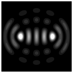
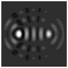
FIG. 3.: Left panel: magnitude of the wavefunction at the Fermi level for the ellipse with $a=71.3\AA$, $e=0.5$. Right panel: Change in the differential conductance due to the impurity at the left focus, - $\delta G(V,\vec{R})$, normalized to the value in the maximum . Scale code: 0.75 - 1 = white, 0 = black, 0-0.75 : grey scale).

The knowledge of the corral spectrum and wavefunctions permits to calculate $G(V,\vec{R})$ for the elliptical corral via equations (5), (6), (9), (13). In figure 3 (right panel), we plot the difference between the $G(V,\vec{R})$ map with and without the impurity, for $eV=0$ [18]. In our calculations we take the value $k_{B}T_{K}=4.6meV$ ($T_{K}=50K$), as observed in [10]. In this experiment $T=4K$, so that condition $T<<T_{K}$ is fulfilled. The change in the differential conductance occurs not only at the focus where the impurity is located but also at the empty focus, located 71 $\AA$ away from the impurity. The fingerprint of the Kondo effect is thus dominantly located around the impurity and around the empty focus. The similitude between the left and the right panel in figure 3 supports our claim that the wavefunction of the corral at the Fermi level projects the Kondo dip from the impurity to the other focus. Our figure 3 should be compared with figures 3-c and 3-d of reference [10]. In the case of surface without corral, the Kondo signature would be localized around the impurity, being negligible at a distance larger than 2$k_{F}^{-1}$ [6].

In figure 4 (left panel) we plot $G(V)$ when the tip is on top of the focus where the impurity is located (compare to figure 4(a) of reference [10]). For this calculation we use $q\approx 0.2$, the value used to fit $G(V)$ without corral [10, 15], and consider a nonzero value for $t_{d}$, following the method outlined in section III. In the right panel of our figure 4 we plot $G(V)$ measured on top of the empty focus. Hence, our theory is in agreement with the main experimental result: the existence of a Kondo resonance at the empty focus, more than 80 $\AA$ away from the magnetic impurity. It must be stressed, however, that in our model the dip observed on top of the magnetic impurity and the one observed on top of the empty focus have different lineshapes, and there exists a factor of 2 between their intensities. In the experiment the attenuation factor is approximately $8$ and both the original dip and the ghost are more symmetric. In order to remove this discrepancy a less phenomenological theory for inelastic processes, like scattering from surface states to bulk states, would be necessary. We predict also that combinations of surface and adatoms for which inelastic scattering is smaller than for Co and Cu would increase the size of the mirage. In figure 5 we also show $G(V)$ when the tip is not at a maximum of the Fermi corral eigenstate. In those situations the mirage is not present, in agreement with the experiments [10].

FIG. 4.: Calculated dips at the focus with a magnetic impurity and at the empty focus of the elliptical corral of figure 3.

FIG. 5.: $G(V)$ at the points $\vec{R}=(25,0)\AA$ (left panel) and $\vec{R}=(35.7,25)$ Å(right panel) of the elliptical quantum corral of figure 3, when a magnetic impurity is placed at the left focus. We take the center of the ellipse as the origin of coordinates.

In figure 6 we plot the intensity of the mirage (the dip amplitude) as a function of $a$, keeping $e=0.5$. In reference [10] an oscillatory dependence of the mirage effect as a function of $a$ (for fixed $e$) was mentioned, the oscillation period being $\lambda_{F}/4$. Our calculation is consistent with that claim. However, we obtain a curve with more structure. The Fourier transform of the intensity of the mirage shows several peaks, the largest of which is located at $\lambda_{F}/4$, in agreement with the experiment. In figure 6 we also plot the number of occupied states inside the corral, as a function of $a$, and keeping $\epsilon_{F}$ constant at 450 meV. We see that most of the changes in the occupation number do not lead to large changes in the mirage strength. The mirage is only enhanced when a particular kind of states, whose wavefunction is heavily peaked very close to the foci, is occupied. This rule was also observed in the experiments [10].

For the ellipse with $e=0.786$ in [10], we have been able to reproduce all the results obtained for the ellipse with $e=0.5$, assuming that the Fermi Level is somewhat below 450 meV. This indicates that the position of the resonances given by the hard wall ellipse might not coincide with the experimental results.

Since the maxima of the Fermi wavefunction are not exactly located at the foci, it is our contention that the important issue is to place the impurity at the maximum of the Fermi wavefunction. Therefore, geometrical or semiclassical interpretations of the mirage might not be adequate to address this phenomenon. To check this, we have studied a square corral, obtaining the mirage effect. Elliptical corrals are very convenient because some states with high quantum numbers (such as the state at the Fermi level for the $e=0.5$ ellipse with the adequate $a$) have two main maxima located close to the foci of the ellipse. In contrast, all the maxima in a square corral have the same height so that the projection effect is less pronounced than in the ellipse.

FIG. 6.: Thick line: Dip amplitude as a function of $a$, $dip(a)$, for an elliptical corral with $e=0.5$. We display $a$ in $\AA$ (upper axis) and in $\lambda_{F}/4$ units (lower axis). Thin line: number of occupied quasi-bound wavefunctions inside the ellipse. In the inset we display the Fourier Transform $f(a_{T})\propto\int_{0}^{\infty}dip(a)\;exp(-i\ 2\pi\ a/a_{T})\;da$ of this curve as a function of the period. We see that the curve peaks at $a_{T}/\frac{\lambda_{F}}{4}=1$.

V Discussion and conclusions

We now comment on some of the limitations of our theory. The first has to do with the approximation of the eigenstates inside the quantum corral as quasi-bound states broadened in energy. For a quantitative description of the corral energy spectrum a more detailed calculation is needed, taking into account the role of the corral atoms as tunneling centers to the bulk states [16]. The second is the use of the Friedel sum rule in a resonant level model. A more realistic calculation of the impurity Green’s function would imply to take into account the real wavefunctions inside the corral and the possibility of tunneling from the magnetic impurity to the bulk states. The quantitative discrepancy with the experiments, in what concerns the attenuation of the mirage, should be solved including these effects. A more complete theory for the STM through magnetic impurities in metallic surfaces without quantum corrals has been developed in [9, 19, 20].

The emphasis of this paper is placed on the qualitative understanding of the mirage rather than on a detailed description of the experiments. Our main results are the following: i) The LDOS evaluated at an arbitrary surface point, $\vec{R}$, in the Anderson model, contains information about the LDOS at the impurity site, $\vec{R}_{I}$. A mirage will appear in a remote point, $\vec{R}$, whenever there is a single quantum state at the Fermi level whose amplitude $\psi_{\epsilon_{F}}$ peaks both at the impurity ($\vec{R}_{I}$) and at $\vec{R}$. In order to avoid destructive interference between different states it is necessary that the energy spacing between states with a non-negligible amplitude at the impurity site is bigger than the energy broadening, $\delta$. ii) The mirage can be obtained in corrals with shapes other than elliptical. However, the elliptical shape is quite convenient because some of the corral eigenstates peak strongly at two points very close to the foci. iii) Our theory predicts that the intensity of the mirage in an elliptical corral oscillates, as a function of the semimajor axis length, keeping fixed the eccentricity, with a dominant period of $\lambda_{F}/4$, in agreement with reference [10].

We want to acknowledge C. Piermarocchi and H. Manoharan for fruitful discussions. JFR and DP acknowledge Spanish Ministry of Education (MEC) for postdoctoral research fellowship and grant FPU/AP98. Work supported in part by MEC under contract PB96-0085.

During the completion of this manuscript we became aware of a theoretical work addressing the problem of the mirage in an elliptical quantum corral [21]. In that work the states of the ellipse are described by a more detailed method, assuming that the wall atoms are magnetic, and the issue of the existence of the mirage in different geometries is not addressed. Our theory can be applied to the general case of a quantum corral formed by non-magnetic scatterers (in which quantum mirages have also been observed [10]).

REFERENCES

- [1] D.M. Eigler and E.K. Schweizer, Nature 344, 524 (1990).
- [2] M.F. Crommie, C.P. Lutz, D.M. Eigler, Nature 363, 524 (1993).
- [3] M.F. Crommie, C.P. Lutz, D.M. Eigler, Science 262, 218 (1993).
- [4] J. Li et al., Phys. Rev. Lett 80, 2893 (1998).
- [5] V. Madhavan et al., Science 280, 567 (1998).
- [6] A.C. Hewson, The Kondo Problem to Heavy Fermions, Cambridge University Press, Cambridge (1997).
- [7] A.A. Abrikosov, Physics 2, 5 (1965). H. Suhl, Phys.Rev. 138, A515 (1965).
- [8] U. Fano, Phys. Rev. 124, 1866 (1961).
- [9] A. Schiller and S. Hershfield, Phys. Rev. B 61, 9036 (2000).
- [10] H.C. Manoharan, C.P. Lutz, D.M. Eigler, Nature 403, 512 (2000).
- [11] P.W. Anderson, Phys. Rev. 124, 41 (1961).
- [12] C. J. Chen, Introduction to Scanning Tunneling Microscopy, Oxford University Press, New York (1993).
- [13] G.D. Mahan, Many Particle Physics, Plenum, 1990.
- [14] W.B. Thimm, J. Kroha and J. von Delft, Phys. Rev. Lett 82, 2143 (1999).
- [15] H. Manoharan, private communication.
- [16] E.J. Heller et al., Nature 369 464 (1994).
- [17] Handbook of mathematical functions, ed. by M. Abramowitz and I. A. Stegun, Dover Publications, New York (1965).
- [18] We have also repeated our calculations considering tunneling from the STM tip to a finite surface in the corral (instead of tunneling to a point). We have obtained very similar results for both cases.
- [19] O. Újsághy et al., condmat/0005166.
- [20] O. Újsághy, G. Zárand and A. Zawadowsky, condmat/0007245.
- [21] O. Agam and A. Schiller, cond-mat/0006443.