Variational Mean Field approach to the Double Exchange Model

Abstract

It has been recently shown that the double exchange Hamiltonian, with weak antiferromagnetic interactions, has a richer variety of first and second order transitions than previously anticipated, and that such transitions are consistent with the magnetic properties of manganites. Here we present a thorough discussion of the variational Mean Field approach that leads to the these results. We also show that the effect of the Berry phase turns out to be crucial to produce first order Paramagnetic-Ferromagnetic transitions near half filling with transition temperatures compatible with the experimental situation. The computation relies on two crucial facts: the use of a Mean Field ansatz that retains the complexity of a system of electrons with off-diagonal disorder, not fully taken into account by the Mean Field techniques, and the small but significant antiferromagnetic superexchange interaction between the localized spins.

75.10.-b, 75.30.Et

]

I Introduction

Doped manganites show many unusual features, the most striking being the colossal magnetoresistance (CMR) in the ferromagnetic (FM) phase [1, 2, 3]. In addition, the manganites have a rich phase diagram as function of band filling, temperature and chemical composition. The broad features of these phase diagrams can be understood in terms of the double exchange model (DEM) [4, 5], although Jahn-Teller deformations [6] and orbital degeneracy may also play a role[7]. A remarkable property of these compounds is the existence of inhomogeneities in the spin and charge distributions in a large range of dopings, compositions and temperatures[8, 9, 10]. In fact, for materials displaying the largest CMR effects, the size of the phase-separated domains is so large ($\sim 0.5\mu\mathrm{m}$ [9]), that the electrostatic stability of the material should be addressed by theorists. At band fillings where CMR effects are present, $x\sim 0.2-0.5$, these compounds can be broadly classified into those with a high Curie temperature and a metallic paramagnetic (PM) phase, and those with lower Curie temperatures and an insulating magnetic phase[11, 12, 13].

The double exchange mechanism was introduced by Zenner [4] through the following Kondo lattice type model

$$H_{\mathrm{K}M}=\sum_{i,j,\alpha}t_{ij}c^{\dagger}_{i\alpha}c_{j\alpha}+J_{\mathrm{H}}\sum_{i,\alpha,\alpha^{\prime}}\mbox{\boldmath$S$}_{i}\cdot c_{i\alpha}^{\dagger}\mbox{\boldmath$\sigma$}_{\alpha\alpha^{\prime}}c_{i\alpha^{\prime}}\,,$$ (1)

where $t$ and $J_{\mathrm{H}}$ are, respectively, $e_{\mathrm{g}}$ electron’s hopping and Hund’s coupling between the $e_{\mathrm{g}}$ and the localized $t_{\mathrm{2}g}$ electrons responsible for the core spin $S$.

When $J_{\mathrm{H}}$ is larger than the width of the conduction band, the model can be reduced to the double exchange model with weak inter-atomic antiferromagnetic (AFM) interactions. Early investigations[14] showed a rich phase diagram, with AFM, canted and FM phases, depending on doping and the strength of the AFM couplings. More recent studies have shown that the competition between the double exchange and the AFM couplings leads to phase separation into AFM and FM regions, suppressing the existence of canted phases[15, 16, 17, 18]. In addition, the double exchange mechanism alone induces a change in the order of the FM transition, which becomes of first order, and leads to phase separation, at low doping[19]. Note, however, that a systematic study of the nature of the transition at finite temperature was not addressed until recently [20], despite its obvious relevance to the experiments. In fact, in Ref.[20] it was shown that a small AFM uniform superexchange interaction between the localized $t_{\mathrm{2}g}$ spins is crucial to understand some of the more relevant features of the phase diagram of the manganites. In particular a first-order phase transition is found between the PM and FM phases in the range $x\sim 0.2-0.5$ is found. This transition does not involve a significant change in electronic density, so that domain formation is not suppressed by electrostatic effects. Therefore, we find a phase-separation of a rather different type of the previously discussed, not driven by a charge instability, but by a magnetic instability. In addition to this phase transition, we recover those previously discussed.

In this work we give a detailed exposition of the new mean-field technique [20] and emphasis is made on the importance of the Berry phase for the existence of first order phase transitions near half filling. We have been able of achieving a more complete description of the phase diagram than in previous work, because we have taken full profit of a very particular feature of the DEM, namely, fermions are bilinearly coupled to classical degrees of freedom (the Mn spins). This allows to trace-out the fermions, thus obtaining a non local effective Hamiltonian for the spins, that can be explicitly written down in terms of the density of states of the fermionic hopping matrix. What we propose to do is to calculate exactly the effective spin-Hamiltonian, for a given (disordered in general) configuration of the spins, using the so called moments-method [21] complemented with an standard truncation procedure [22]. This technique can be directly used for other models, like for instance models of classical spins and lattice vibrations coupled to fermions without direct interactions [6], or also in contexts different from the manganites physics like the pyrochlores or double perovskytes. Once electrons are traced-out, we study the spin thermodynamics using the variational version of the Weiss Mean-Field method [23].

The main difference of our approach with previous work is in that we use the exact spin-Hamiltonian, while an approximated form was used up to now. For instance, the effective crystal approximation, which amounts to consider that electrons move on a perfect crystal, with a magnetically reduced hopping, was employed in [14] (see section VIII for a comparison with our method). A more accurate estimate of the density of states, well-known from the physics of disordered-systems and which becomes exact on the infinite dimensions limit [19], is the CPA. Notice that for non self-interacting electrons the Dynamical Mean-Field Approximation(DMFA) [24, 25] is also equivalent to a CPA calculation on a given mean-field, which is determined via self-consistency equations (both the mean-field and the CPA density of states are obtained self-consistently). Although those approaches are reasonable, and provide useful information, they are approximated in two different ways, which is undesiderable because two different effects are entangled. First, even for only-spins models of magnetism (like the Ising Model) where the exact spin Hamiltonian can be evaluated easily, the Mean-Field approximation neglects the spatial correlations of the statistical fluctuations of the order parameter (see e.g. [23]). But, in addition, for an electron-mediated magnetic interaction, the evaluation of the effective spin Hamiltonian is only accurate in the limit of infinite dimensions. With our approach, the correlations on the magnetic fluctuations are to be blamed for all the differences between our results and the real behavior of the model. On the other hand, in section VIII we show how the failure of the effective-crystal approximation on finding the first-order phase transition at half-filling is due to the inaccuracy on the calculation of the density of states. Moreover, we are able to study directly in three dimensions some rather subtle details, like the non-negligible effects of keeping the Berry phase on the DEM Hamiltonian.

The structure of the paper is as follows. In Section II we introduce the DEM and our notations. In Section III we present our Mean-Field approximation. The very non-trivial part of the work, the computation of the Density of States, is explained in Section IV. It requires numerical simulations that can be performed on large lattices with a high accuracy. They are described in Section V. The effects of the Berry phase are analyzed in Section VI. Section VII is devoted to the study of the influence of the Berry phase in the phase diagram of the DEM. The comparison of the Mean-Field approach studied in this work with the de Gennes’s [14] and with the DMFA is carried out in Section VIII. The conclusions are summarized in Section IX.

II Model

We study a cubic lattice with one orbital per site. At each site there is also a classical spin. The coupling between the conduction electron and this spin is assumed to be infinite, so that the electronic state with spin antiparallel to the core spin can be neglected. Finally, we include an AFM coupling between nearest neighbor core spins. We neglect the degeneracy of the conduction band. Thus, we cannot analyze effects related to orbital ordering, which can be important in the highly doped regime, $x>0.5$[7, 26] (see however Ref. [27]). We also neglect the coupling to the lattice. We focus on the role of the magnetic interactions only. As mentioned below, magnetic couplings suffice to describe a number of discontinuous transitions in the regime where CMR effects are observed. These transitions modify substantially the coupling between the conduction electrons and the magnetic excitations. Thus, they offer a simple explanation for the anomalous transport properties of these compounds. Couplings to additional modes, like optical or acoustical phonons, will enhance further the tendency towards first order phase transitions. We consider that a detailed understanding of the role of the magnetic interactions is required before adding more complexity to the model. Note that there is indeed evidence that, in some compounds, the coupling to acoustical phonons[28] or to Jahn-Teller distortions[29] is large.

The Hamiltonian of the DEM is

$${\cal H}=\sum_{ij}{\cal T}(\mbox{\boldmath$S$}_{i},\mbox{\boldmath$S$}_{j})c_{i}^{\dagger}c_{j}+\sum_{ij}\tilde{J}_{\mathrm{A}F}S^{2}\mbox{\boldmath$S$}_{i}\cdot\mbox{\boldmath$S$}_{j}$$ (2)

where $S=3/2$ is the value of the spin of the core, Mn³⁺, and $S$ stands for a unit vector oriented parallel to the core spin, which we assume to be classical. In the following, we will use $J_{\mathrm{A}F}=\tilde{J}_{\mathrm{A}F}S^{2}$. Calculations show that the quantum nature of the core spins does not induce significant effects[17]. In one of the earliest studies of this model [14], the superexchange coupling was chosen FM between spins lying on the same $z=constant$ plane, and AFM between spins located on neighboring planes. This is a reasonable starting point for the study of ${\mathrm{L}a}_{1-x}{\mathrm{C}a}_{x}{\mathrm{M}n}{\mathrm{O}}_{3}$ if $x<0.16$, where A-type antiferromagnetism is found. For larger doping, $0.16<x<0.5$, which is our main focus, the magnetism is uniform and there is no a priori reason for favoring a particular direction.

The function

$${\cal T}(\mbox{\boldmath$S$}_{i},\mbox{\boldmath$S$}_{j})=t\left[\cos\frac{\theta_{i}}{2}\cos\frac{\theta_{j}}{2}+\sin\frac{\theta_{i}}{2}\sin\frac{\theta_{j}}{2}{\mathrm{e}}^{{\mathrm{i}}(\varphi_{i}-\varphi_{j})}\right]$$ (3)

stands for the overlap of two spin 1/2 spinors oriented along the directions defined by $\mbox{\boldmath$S$}_{i}$ and $\mbox{\boldmath$S$}_{j}$, whose polar and azimuthal angles are denoted by $\theta$ and $\varphi$, respectively. It defines a hopping matrix ${\cal T}$, whose matrix elements are ${\cal T}_{ij}={\cal T}(\mbox{\boldmath$S$}_{i},\mbox{\boldmath$S$}_{j})$. The hopping function can be written as

$${\cal T}(\mbox{\boldmath$S$}_{i},\mbox{\boldmath$S$}_{j})=t\cos\frac{\vartheta_{ij}}{2}\exp({\mathrm{i}}\phi_{ij})\,,$$ (4)

where $\vartheta_{ij}$ is the relative angle between $\mbox{\boldmath$S$}_{i}$ and $\mbox{\boldmath$S$}_{j}$, and $\phi_{ij}$ is the so called Berry phase. It is sometimes assumed that the Berry phase can be set to zero without essential loss. It is therefore interesting to study the model that ignores the Berry phase, the hopping matrix being

$${\cal T}^{\mathrm{m}od}_{ij}=\left|{\cal T}_{ij}\right|=\cos\frac{\vartheta_{ij}}{2}=\sqrt{\frac{1+\mbox{\boldmath$S$}_{i}\cdot\mbox{\boldmath$S$}_{j}}{2}}\,.$$ (5)

In the following sections we will analyze both models, with Berry phase (hopping matrix ${\cal T}$) and without Berry phase (hopping matrix ${\cal T}^{\mathrm{m}od}$).

III Mean-field approximation

Our approach to the problem follows the variational formulation of the Mean-Field approximation, described for instance in [23]. We start by writing the Grand Canonical partition function for the DEM:

$${\cal Z}_{\mathrm{G}C}=\int[dS]{\mathrm{T}r}^{\mathrm{(}Fock)}\exp\left[-({\cal H}-\mu{\cal N})/T\right]\,,$$ (6)

where $\mu$ is the electronic chemical potential, ${\cal N}=\sum_{i}c_{i}^{\dagger}c_{i}$ is the electron number operator, $T$ is the temperature and we use units in which the Boltzmann constant is one. The trace, taken over the electron Fock space, defines an effective Hamiltonian for the spins,

$$\exp\left[-{\cal H}^{\mathrm{e}ff}(\mbox{\boldmath$S$})/T\right]={\mathrm{T}r}^{\mathrm{(}Fock)}\exp\left[-({\cal H}-\mu{\cal N})/T\right]\,,$$ (7)

that can be computed in terms of the eigenvalues, $E_{n}$, of the hopping matrix, ${\cal T}$:

$${\cal H}^{\mathrm{e}ff}(\mbox{\boldmath$S$}) = J_{\mathrm{A}F}\sum_{\langle ij\rangle}\mbox{\boldmath$S$}_{i}\cdot\mbox{\boldmath$S$}_{j}-$$ (9)

$$T\sum_{n}\log\left\{1+\exp\left[-(E_{n}(\mbox{\boldmath$S$})-\mu)/T\right]\right\}\,.$$

Introducing the Density of States (DOS) of ${\cal T}$:

$$g(E;\mbox{\boldmath$S$})=\frac{1}{V}\sum_{n=1}^{V}\delta\left[E-E_{n}(\mbox{\boldmath$S$})\right]\,,$$ (10)

where $V$ is the volume of the lattice, the effective Hamiltonian can be written as

$${\cal H}^{\mathrm{e}ff}(\mbox{\boldmath$S$}) = \sum_{\langle ij\rangle}J_{\mathrm{A}F}\mbox{\boldmath$S$}_{i}\cdot\mbox{\boldmath$S$}_{j}-$$ (12)

$$TV\int dE\,g(E;\mbox{\boldmath$S$})\log\left[1+e^{-(E-\mu)/T}\right]\,.$$

The Grand Canonical partition function becomes an integral in spin configuration space:

$${\cal Z}_{\mathrm{G}C}=\int[dS]\exp\left[-{\cal H}_{\mathrm{e}ff}(\mbox{\boldmath$S$})/T\right]\,.$$ (13)

Thermodynamics follows from Eq. (13) as usual. The free energy, ${\cal F}$, and the electron density, $x$, are given by:

$${\cal F}=-\frac{T}{V}\log{\cal Z}_{\mathrm{G}C}$$ (14)

$$x=\frac{\partial{\cal F}}{\partial\mu}=\int dE\,\langle g(E;\mbox{\boldmath$S$})\rangle\frac{1}{1+\exp\left[(E-\mu)/T\right]}$$ (15)

where $\langle\cdots\rangle$ stands for spectation value over equilibrium spin configurations.

The variational Mean-Field approach consist on comparing the actual system with a set of simpler reference models, whose Hamiltonians, ${\cal H}_{\mbox{\boldmath$h$}}$, depend on external parameters, $\mbox{\boldmath$h$}_{i}$. For simplicity, we choose the model:

$${\cal H}_{\mbox{\boldmath$h$}}=-\sum_{i}\mbox{\boldmath$h$}_{i}\cdot\mbox{\boldmath$S$}_{i}\,.$$ (16)

The variational method is based on the inequality

$${\cal F}\leq{\cal F}_{\mbox{\boldmath$h$}}+\left\langle{\cal H}^{\mathrm{e}ff}-{\cal H}_{\mbox{\boldmath$h$}}\right\rangle_{\mbox{\boldmath$h$}},$$ (17)

where ${\cal F}_{\mbox{\boldmath$h$}}$ is the free energy of the system with Hamiltonian (16), and the expectation values $\langle\cdots\rangle_{\mbox{\boldmath$h$}}$ are calculated with the Hamiltonian ${\cal H}_{\mbox{\boldmath$h$}}$. The inequality (17) follows easily from the concavity of the exponential function [23]. The best approximation to the actual free energy with the ansatz of Eq. (16) is

$${\cal F}=\min_{\mbox{\boldmath$h$}}\left\{{\cal F}_{\mbox{\boldmath$h$}}+\left\langle{\cal H}^{\mathrm{e}ff}\right\rangle_{\mbox{\boldmath$h$}}-\left\langle{\cal H}_{\mbox{\boldmath$h$}}\right\rangle_{\mbox{\boldmath$h$}}\right\}\,.$$ (18)

Since, for technical reasons that will become clear in the following, it is not possible to work with one field $\mbox{\boldmath$h$}_{i}$ per site, we must select some subsets that contain only a few independent parameters (see Section VII). The choice is of paramount importance since it is an ansatz that will artificially restrict the behavior of the system. We have chosen the following four families [30] of fields, depending on a parameter, $h$:

$$\mbox{\boldmath$h$}_{i} = \mbox{\boldmath$h$}\,,$$ (19)

$$\mbox{\boldmath$h$}_{i} = (-1)^{z_{i}}\mbox{\boldmath$h$},$$ (20)

$$\mbox{\boldmath$h$}_{i} = (-1)^{x_{i}+y_{i}}\mbox{\boldmath$h$},$$ (21)

$$\mbox{\boldmath$h$}_{i} = (-1)^{x_{i}+y_{i}+z_{i}}\mbox{\boldmath$h$}\,,$$ (22)

which correspond, respectively, to FM, A-AFM, C-AFM, and G-AFM orderings. There is an order parameter (magnetization) associated to each of these orderings. We will denote them by $M_{\mathrm{F}}$, $M_{\mathrm{A}}$, $M_{\mathrm{C}}$, and $M_{\mathrm{G}}$, respectively. As a shorthand, they will be denoted generically by ${\cal M}$. The order parameter is related to the corresponding $h$ by

$${\cal M}=\frac{1}{\tanh h}-\frac{1}{h}\,,$$ (23)

where $h=|\mbox{\boldmath$h$}|/T$. Thus, the free energy can be written in terms of ${\cal M}$ instead of $h$ and Eq. (18) implies that it must be minimized with respect to $\cal M$. The free energy has three contributions: the fermion free energy (FFE), the superexchange energy and the entropy of the spins:

$${\cal F}({\cal M})={\cal F}_{\mathrm{F}er}({\cal M})+NJ_{\mathrm{AF}}{\cal M}^{2}-T{\cal S}_{\mbox{\boldmath$h$}}({\cal M})\,,$$ (24)

where $N$ is , respectively, 3,$-3$, 1 and $-1$ for FM, G-AFM, A-AFM and C-AFM orderings.

The entropy of the spins can be easily computed in terms of the Mean-Field:

$${\cal S}_{\mbox{\boldmath$h$}}({\cal M}) = ({\cal F}_{\mbox{\boldmath$h$}}-\left\langle{\cal H}_{\mbox{\boldmath$h$}}\right\rangle_{\mbox{\boldmath$h$}})/T$$ (25)

$$= \log\left[\sinh h({\cal M})/h({\cal M})\right]-h({\cal M}){\cal M}\,,$$ (26)

but the FFE,

$${\cal F}_{\mathrm{F}er}({\cal M})=-T\int dE\,\left\langle g(E;\mbox{\boldmath$S$})\right\rangle_{\mbox{\boldmath$h$}}\log\left[1+{\mathrm{e}}^{-(E-\mu)/T}\right]\,,$$ (27)

must be estimated numerically.

The non trivial part of the computation is the average of the DOS $\langle g(E;\mbox{\boldmath$S$})\rangle_{\mbox{\boldmath$h$}}$. The key is that it can be computed by numerical simulations on large lattices with high accuracy, ought to two basic facts: 1) the Mean Field Hamiltonian (16) describes uncorrelated spins and therefore equilibrium spin configurations can be easily generated on very large lattices, and 2) the DOS is a self-averaging quantity. This last point means that the mean value of the DOS can be obtained on a large lattice by averaging it over a small set of equilibrium configurations. Once the DOS is computed, the integral of Eq. (27) can be performed numerically to get the FFE as a function of ${\cal M}$.

IV Computation of the averaged DOS

The DOS can be accurately computed for any given spin configuration with the technique that we describe in the following [21]. From its definition, Eq. (10), the DOS is a probability distribution in the variable $E$, whose moments are

$$\mu_{k}(\mbox{\boldmath$S$})=\int dE\,g(E;\mbox{\boldmath$S$})E^{k}=\frac{1}{V}{\mathrm{T}r}{\cal T}^{k}$$ (28)

Now, it is easy to show that the eigenvalues of the hopping matrix verify $-6t\leq E_{n}<6t$. A probability distribution of compact support can be reconstructed from its moments using the techniques of Stieljes [31]. In practice, we only know the first $p$ moments, but the method of Stieljes allows us to find a good approximation to the distribution if $p$ is large enough.

To compute the averaged DOS we follow four steps:

• Generate spin configurations, $\left\{\mbox{\boldmath$S$}\right\}$, according to the Mean-Field Boltzmann weight, $\exp(-{\cal H}_{\mbox{\boldmath$h$}}/T)$. This can be achieved very efficiently with a heat bath algorithm, since all the spins are decoupled in the Mean-Field Hamiltonian. In this way, one obtains spin configurations in perfect thermal equilibrium with the Boltzmann-weight given by the Mean-Field Hamiltonian.

• For each $\left\{\mbox{\boldmath$S$}\right\}$, one would calculate the moments of the DOS, using Eq. (28), and then apply the techniques of reconstruction of Stieljes [31]. However, this is impractical since, although the matrix ${\cal T}$ is sparse, the trace in Eq. (28) would require to repeat the process $V$ times, and we would end-up with an algorithm of order $V^{2}$. We use instead an stochastic estimator. First, we extract a normalized random vector $|v\rangle$, with components

  $$v_{i}=\frac{\alpha_{i}}{\sum_{j=0}^{V}\alpha_{j}^{2}}\,$$ (29)

  where the $\alpha_{i}$ are random numbers extracted with uniform probability between $-1$ and $1$. Let us now call $|n\rangle$ to the eigenvector of eigenvalue $E_{n}$ of the matrix ${\cal T}$. It is easy to check that (the overline stands for the average on the random numbers $\alpha_{i}$)

  $$\overline{v_{i}v_{j}} = \frac{\delta_{i,j}}{V}\,,$$ (30)

  $$\overline{\langle n|v\rangle\langle v|m\rangle} = \frac{\delta_{n,m}}{V}\,.$$ (31)

  Then we introduce a $v$-dependent density of states:

  $$g(E;v;\mbox{\boldmath$S$})\equiv\sum_{n=1}^{V}\,|\langle n|v\rangle|^{2}\,\delta(E-E_{n})\,.$$ (32)

  From Eq. (31), it follows immediately that

  $$\overline{g(E;v;\mbox{\boldmath$S$})}=g(E;\mbox{\boldmath$S$})\,.$$ (33)

  From $\langle v|v\rangle=1$, and from Eq. (32), we see that $g(E;v;\mbox{\boldmath$S$})$ is a perfectly reasonable distribution function, whose moments are

  $$\int\,dE\ E^{k}\,g(E;v;\mbox{\boldmath$S$})=\langle v|{\cal T}^{k}|v\rangle$$ (34)

  Numerically, the algorithm is of order $k\times V$, since, as mentioned, ${\cal T}$ is sparse and only $O(V)$ operations are required to multiply $v$ by ${\cal T}$. This method allows to compute a large number of moments on large lattices. However, notice that the actual calculation is not performed this way (round-off errors would grow enormously with the power of ${\cal T}$), but as explained in the appendix.

• Reconstruct $g(E;v;\mbox{\boldmath$S$})$ from the moments, by the method of Stieljes. The DOS is obtained in a discrete but very large number of energies, $E$. The cost of refining this set of energies is negligible. Hence, the integral over $E$ that gives the FFE, Eq. (27), can be approximated numerically with high accuracy.

• Average $g(E;v;\mbox{\boldmath$S$})$ over the spin configurations $S$ and over the random vectors $|v\rangle$. In practice we only use a random vector per spin configuration: it is useless to obtain an enormous accuracy on the density of states for a particular spin configuration, that should be spin-averaged, anyway. Since the errors due to the fluctuations of the spins and the fluctuations of the $|v\rangle$ are statistically uncorrelated, both of them average out simultaneously [32]. It is crucial that the DOS is a self-averaging quantity, what means that its fluctuations are suppressed as $1/\sqrt{V}$. Hence, its average over a few equilibrium configurations is enough to estimate it with high accuracy.

This program can be carried out successfully on lattices as large as $64^{3}$ and even $96^{3}$, computing a large enough number of moments, $50$ or $75$. As we shall see, this suffices to achieve an excellent accuracy in the averaged DOS and in the FFE.

The whole process is repeated for several values of the Mean Fields $h$ within each family. The FFE computed in a discrete set of magnetizations is extended to a continuous function of ${\cal M}$ in the interval $[0,1]$ through a polynomial fit, as we will show in next section. The magnetic phase diagram of the model will come out easily then.

V Extracting the Fermionic Free Energy

Let us discuss in this section the numerical results for the averaged DOS and for the FFE. We carried out the program designed in the previous section for 20 values of $h$ within each family of Mean Fields, chosen in such a way that the corresponding magnetizations, $\cal M$, are uniformly distributed in $[0,1]$. The expectation value $\langle g(E;\mbox{\boldmath$S$})\,\rangle_{\mbox{\boldmath$h$}}$ is estimated by averaging over 50 equilibrium (with respect to the Mean Field distribution) spin configurations. This is enough to have the statistical errors under control on a $64^{3}$ lattice.

FIG. 1.: Averaged DOS, reconstructed with 50 moments, versus $E$, for four values of the mean-field corresponding to $M_{\mathrm{F}}=1$ (solid line), $M_{\mathrm{F}}=0.5$, (dashed line), paramagnetic (dotted line), and $M_{\mathrm{G}}=0.5$, (dot-dashed line).

Figure 1 displays the averaged DOS, computed on a $64^{3}$ lattice for four values of $h$, corresponding to FM, ($M_{\mathrm{F}}=0.5$ and $M_{\mathrm{F}}=1$), paramagnetic, and G-AFM ($M_{\mathrm{G}}=0.5$) phases. They were reconstructed with its 50 first moments [33]. Note that the DOS is even in $E$, as required by the the particle-hole symmetry, and that it becomes narrower in going from the FM to the G-AFM phase, as expected. The width of the density of states in the PM phase is $8t$, two thirds of the width corresponding to the perfect ferromagnetic, in agreement with the results of full diagonalization [34].

From the averaged DOS it is straightforward to compute the FFE by performing the integral entering Eq. (27) numerically. In this way, we computed ${\cal F}_{\mathrm{F}er}$ for the chosen values of ${\cal M}$. Given that the free energy can be shifted by a term independent of ${\cal M}$, we use ${\cal F}_{\mathrm{F}er}({\cal M})-{\cal F}_{\mathrm{F}er}(0)$ instead of ${\cal F}_{\mathrm{F}er}({\cal M})$ [35].

To have an analytic expression for ${\cal F}_{\mathrm{F}er}$, we fit the data with a polynomial of order sixth in ${\cal M}$ , with coefficients that depend on $T$ and $\mu$:

$${\cal F}_{\mathrm{F}er}^{(I)}(M_{I})\;=\;A_{2}^{(I)}\,M_{I}^{2}\>+\>A_{4}^{(I)}\,M_{I}^{4}\>+\>A_{6}^{(I)}\,M_{I}^{6}\,.$$ (35)

The index $I$ denotes the type of ordering: $I\,=\,{\mathrm{F},A,C}$, or ${\mathrm{G}}$.

Figure 2 shows the FFE at $T=0$ and $\mu=0$, which correspond to half filling, $x=1/2$, as a function of $M_{\mathrm{F}}$ or $M_{\mathrm{G}}$. The points are the result of the numerical computation and the lines are the best fits of the form (35). The high quality of the fits is remarkable. Note that the fermions favor FM order. The coefficients $A_{j}^{(I)}(T,\mu)$ of Eq. (35), which will play a major role in the exploration of the phase diagram, are displayed in Figure 3 in the cases $I={\mathrm{F},G}$, for $T=0$, as a function of $\mu$. We always found $A_{2}^{\mathrm{(}F)}(T,\mu)<0$ and $A_{2}^{\mathrm{(}G)}(T,\mu)>0$, in agreement with the FM nature of the spin interaction induced by the double exchange mechanism.

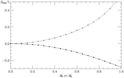
FIG. 2.: FFE at $T=0$ and $\mu=0$ ($x=1/2$) versus $M_{\mathrm{F}}$ (squares, solid line) or $M_{\mathrm{G}}$ (circles, dotted line). The points are the results of the simulation and the lines are the three parameter fit.

FIG. 3.: Coefficients $A_{2}^{\mathrm{(}F)}$, $A_{2}^{\mathrm{(}G)}$, $A_{4}^{\mathrm{(}F)}$, $A_{4}^{\mathrm{(}G)}$, $A_{6}^{\mathrm{(}F)}$, and $A_{6}^{\mathrm{(}G)}$ of the fits (35) versus $\mu$, at $T=0$. Each figure contains four lines (that sometimes cannot be distinguished) corresponding to the four different computations mentioned in the text, three with 50 and one with 75 moments.

Let us estimate the errors of our numerical approach. We have three sources of errors:

• Finite size of the lattice.

• Statistics, arising from the numerical simulation.

• Truncation of the infinite sequence of moments.

Finite size errors have been estimated comparing the results on a $64^{3}$ and a $96^{3}$ lattice. They turn out to be negligible, as expected given the sizes of the lattices. To estimate the statistical errors we performed three different simulations using the 50 lowest order moments. One more simulation, this time with the 75 first moments, was done in order to study the systematic error associated to the truncation of the sequence of moments. As an example, Figure 4 displays the averaged DOS in the FM phase $(M_{\mathrm{F}}=0.5)$ extracted from two different simulations, one with 50 and the other with 75 moments. We see only tiny differences, which can hardly be appreciated on the scale of the figure. This small error propagates to the FFE, which is shown in Figure 5 for $T=0$ and $\mu=0$. There are four sets of points plotted, corresponding to the four mentioned simulations. Again, the differences cannot be appreciated. The errors in the computed FFE give rise to uncertainties in the coefficients $A$’s of Eq. (35), which can be appreciated in Fig. 3. The largest errors appear at $\mu=0$ (half-filling). We have also checked that fits to a polynomial of eight-order do not change the values of $A_{j}^{(I)}$ significantly. FIG. 4.: Averaged DOS vs. energy for $M_{\mathrm{F}}=0.5$ on a $64^{3}$ lattice from a simulation using 50 moments (solid line) and another one with 75 moments (dashed). The curves can hardly be distinguished on this scale.

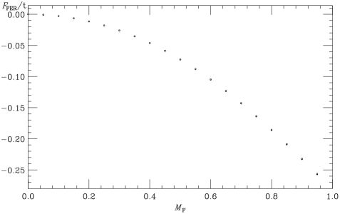
FIG. 5.: Fermion free energy vs. $M_{\mathrm{F}}$ from four simulations on a $64^{3}$ lattice. Three of them, carried out to estimate the statistical errors, used 50 moments to reconstruct the DOS. The other one, aimed to estimate the systematic errors due to the truncation of the sequence of moments, took into account 75 moments. The errors turn out to be so small that cannot be appreciated on the scale of the figure.

To summarize, we have checked that the numerical uncertainties inherent to our numerical approach are well under control and therefore all the conclusions are robust in this sense. The discrepancies between our analysis and the true behavior of the system, if they are important, must be attributed only to the Mean-Field ansatz.

VI Effect of the Berry phase

Sometimes it is stated that one can ignore the Berry phase in the DEM without loosing anything important. To investigate this point, let us repeat our analysis of the DEM setting the Berry phase to zero. All we have to do is to compute the DOS of the hopping matrix ${\cal T}^{\mathrm{m}od}_{ij}$ of Eq. (5). The rest is identical to what we have discussed in the previous sections.

FIG. 6.: Averaged DOS in the paramagnetic phase ($M_{\mathrm{F}}=0$, upper panel) and in the ferromagnetic phase ($M_{\mathrm{F}}=0.5$, lower panel) with (solid) and without (dashed) Berry phase.

Figure 6 displays the averaged DOS at $M_{\mathrm{F}}=0$ (PM phase) and $M_{\mathrm{F}}=0.5$ for hopping with and without Berry phase. At first sight, the differences, although noticeable (they are much bigger than the errors, cf. Fig. 4), do not seem very important. However, it happens that the results are very sensitive to small modifications of the DOS. We shall see indeed that the presence or absence of the Berry phase is crucial for some features of the phase diagram. Thus, the analysis of errors of the previous section turns out to be extremely important to give a meaning to our results. Notice that the effect of the Berry phase is stronger in the disordered phase, as expected.

FIG. 7.: Fermion free energy at $T=0$ and $\mu=0$ as a function of $M_{\mathrm{F}}$ with (solid) and without (dashed) Berry phase. Notice that, in both cases, the free energy has been taken vanishing at the origin by convention.

Figure 7 shows the effects of the Berry phase on the FFE at $T=0$ and $\mu=0$. These effects modify the coefficients $A_{k}^{(I)}$ entering ${\cal F}_{\mathrm{F}er}$, which can be seen in Fig. 8. These coefficients are very sensitive to the modifications of the DOS induced by the Berry phase. Of especial relevance is $A_{4}^{\mathrm{(}F)}$, which, as we shall see in the next section, governs the possibility of having first order PM-FM transitions. In particular, in the vicinity of $\mu=0$ this coefficient is negative. Notice however that without the Berry phase $A_{4}^{(I)}$ is negative around $\mu=0$ in a smaller region than with Berry phase, and it is closer to zero. This fact induces important differences in the nature of the phase transitions of the model, as we shall see in the next section.

VII Phase diagram

The equilibrium states are determined by the absolute minima of the free energy, Eq. (24), respect to the order parameters, ${\cal M}$. The minima determine the phases and the phase boundaries. Given that we know ${\cal F}$ as a function of ${\cal M}$, the problem of determining the equilibrium states is reduced to numerical minimization of a function of a single variable. This is indeed the way we proceed. It is however illuminating to get some insight by a semi-analytic treatment of the problem. As we have seen, to a very good approximation, the FFE is a polynomial of sixth degree in ${\cal M}$. The entropy (26) can also be expanded in powers of ${\cal M}$ around ${\cal M}=0$:

$${\cal S}_{\mbox{\boldmath$h$}}({\cal M})=-\left(\frac{3}{2}{\cal M}^{2}+\frac{9}{20}{\cal M}^{4}+\frac{99}{350}{\cal M}^{6}+\ldots\right)\,.$$ (36)

Hence, we find the Landau expansion of the free energy in powers of the order parameter:

$${\cal F}({\cal M})=c_{2}{\cal M}^{2}+c_{4}{\cal M}^{4}+c_{6}{\cal M}^{6}+\ldots\,.$$ (37)

FIG. 8.: Coefficients of the fit (35) of the fermion free energy at $T=0$ as a function of $\mu$ with (solid) and without (dashed) Berry phase.

The coefficients of the expansion are

$$c_{2} = \frac{3}{2}T\>+\>NJ_{\mathrm{A}F}\>+\>A_{2}^{(I)}(T,\mu)\,,$$ (38)

$$c_{4} = \frac{9}{20}T\>+\>A_{4}^{(I)}(T,\mu)\,,$$ (39)

$$c_{6} = \frac{99}{350}T\>+\>A_{6}^{(I)}(T,\mu)\,,$$ (40)

where $N$ was defined right after Eq. (24).

The free energy has the symmetry ${\cal M}\rightarrow-{\cal M}$. At high $T$, the entropic term dominates and the minimum of ${\cal F}$ is at ${\cal M}=0$. As the temperature decreases, the internal energy becomes more important and the absolute minimum of ${\cal F}$ can be located at ${\cal M}\neq 0$. The phase transition will be continuous when the absolute minimum at the origin changes to a maximum, i.e.:

$$c_{2}\;=\;0\hskip 7.11317pt\Longrightarrow\hskip 7.11317pt\frac{3}{2}T_{\mathrm{c}}\>+\>NJ_{\mathrm{A}F}\>+\>A_{2}^{(I)}(T_{\mathrm{c}},\mu)\;=\;0$$ (41)

At a first order transition three minima, ${\cal M}=0$ and ${\cal M}=\pm{\cal M}_{0}\neq 0$, are degenerate. Three conditions must hold:

• Minimum at ${\cal M}=0$:

  $$c_{2}>0\,.$$ (42)

• Minimum at ${\cal M}_{0}$:

  $$2c_{2}+4c_{4}{\cal M}_{0}^{2}+6c_{6}{\cal M}_{0}^{4}=0\,.$$ (43)

• Degeneracy (${\cal F}(0)={\cal F}({\cal M}_{0})$):

  $$c_{2}+c_{4}{\cal M}_{0}^{2}+c_{6}{\cal M}_{0}^{4}=0\,.$$ (44)

FIG. 9.: Phase diagram of the DEM in the plane $(x,T/t)$, for several values of $J_{\mathrm{A}F}/t$. The left (right) part corresponds to the model with (without) Berry phase. Solid (dashed) lines represent first (second) order transitions and the zones with stripes are phase separation regions. The onset for first order PM-FM transition is at $J_{\mathrm{A}F}\approx 0.06$ in the model with Berry phase, while such transitions do not appear if the Berry phase is neglected.

The solution of these three equations is:

$${\cal M}_{0}^{2}=-2c_{2}/c_{4}$$ (45)

$$c_{6}=c_{4}^{2}/(4c_{2})$$ (46)

$$c_{2}>0;\hskip 14.22636ptc_{4}<0;\hskip 7.11317ptc_{6}>0$$ (47)

Eq. (45) gives the spontaneous magnetization; Eq. (46) determines the critical temperature $T_{\mathrm{c}}$ of the first order transition as a function of $\mu$ and $J_{\mathrm{A}F}$; Eq. (47) sets necessary conditions (real ${\cal M}_{0}$) for a first order transition to happen. We see that to have a first order PM-FM transition we must have $A_{4}^{(I)}(T_{\mathrm{c}},\mu)<0$. Fig. 3 shows that in particular this is possible around half filling.

The boundaries between first and second order lines are tricritical points. They are determined by the conditions:

$$c_{2}=0\hskip 14.22636pt \Longrightarrow \hskip 14.22636ptJ_{\mathrm{A}F}^{\mathrm{t}}=-\frac{3}{2N}T_{\mathrm{t}}-\frac{A_{2}^{(I)}(T_{\mathrm{t}},\mu)}{N}$$ (48)

$$c_{4}=0\hskip 14.22636pt \Longrightarrow \hskip 14.22636ptT_{\mathrm{t}}=-\frac{20}{9}A_{4}^{(I)}(T_{\mathrm{t}},\mu)\hskip 42.67912pt$$ (49)

With these ingredients, we are able to discuss the phase diagram of the DEM. It has been shown in [20] that the phase diagram of double exchange systems is richer than previously anticipated and differs substantially from that of more conventional itinerant ferromagnets. Moreover, it is consistent with the magnetic properties of manganites [8, 9, 10, 11, 12, 13, 36, 37, 38] (see section IX).
FIG. 10.: Phase diagram of the DEM without Berry phase in the plane $(x,J_{\mathrm{A}F})$ at $T=0$. We shall not repeat here the analysis of the phase diagram of the DEM carried out in [20]. Let us concentrate on the effects of the Berry phase. Figure 9 displays the phase diagram in the plane $(x,T/t)$, for several values of $J_{\mathrm{A}F}$. The left part corresponds to the model that includes the Berry phase and on the right the Berry phase is neglected. For $J_{\mathrm{A}F}<0.06$ both phase diagrams are very similar. The transition temperature is slightly higher (13%) at half filling in the model that ignores the Berry phase. At low filling, both phase diagrams are almost identical. However, for $J_{\mathrm{A}F}>0.06$ important differences arise. A first order PM-FM transition develops around half filling if the Berry phase is taken into account. The onset for such behavior is $J_{\mathrm{A}F}=0.06$. In contrast, the PM-FM transition around half filling remains continuous for any value of $J_{\mathrm{A}F}$ if the Berry phase is neglected. The explanation is simple: the coefficient $A_{4}^{\mathrm{(}F)}$, although negative, has a too small absolute value to drive a first order transition. This negative coefficient would become effective if the critical temperature were much lower, what can be achieved by increasing the AF superexchange coupling. But in this case the competition between FM and AF is so strong that the transition at half filling takes place between PM and A-AFM phases, and it is second order. First order PM-FM transitions only appear if the Berry phase is properly taken into account.

At $T=0$, the phase diagrams are similar in both cases, and we only display that of the model without Berry phase, in Fig. 10. The discussion of [20] applies to this case without any modification.

Let us end this section with the analysis of the phase transitions at finite applied magnetic field, $B$. The first order PM-FM transition around half filling survives under an applied magnetic field. In this case, the order parameter, $M_{\mathrm{F}}$, is non-zero in both phases, but suffers a jump on a line in the plane $(B,T)$. The line ends at a critical point, $(B^{*},T^{*})$, which has a certain magnetization $M_{\mathrm{F}}^{*}$. The critical field can be measured and is of interest [39, 40]. Let us compute it. The free energy in the presence of a magnetic field, $B$, is:

$${\cal F}(M_{\mathrm{F}})\;=\;c_{2}M_{\mathrm{F}}^{2}\>+\>c_{4}M_{\mathrm{F}}^{4}\>+\>c_{6}M_{\mathrm{F}}^{6}\>-\>BM_{\mathrm{F}}\,.$$ (50)

The magnetic field shifts the three degenerate minima of the zero-field PM-FM first order transition and lifts the degeneracy. By tuning (increasing) the temperature it is possible to get two degenerate minima again, and a first order transition takes place. In this way, we get a transition line in the $(B,T)$ plane. Increasing $B$, the two degenerate minima become closer. At the critical field, $B^{*}$, both minima coalesce at some point $M_{\mathrm{F}}^{*}$, and the transition disappears. When this happens, the three first derivatives of ${\cal F}$ respect $M_{\mathrm{F}}$ vanish, and the fourth is positive. These conditions read:

$${\cal F}^{\prime}(M_{\mathrm{F}}^{*})=0 \Rightarrow B^{*}=2c_{2}M_{\mathrm{F}}^{*}+4c_{4}M_{\mathrm{F}}^{*\,3}+6c_{6}M_{\mathrm{F}}^{*\,5}$$ (51)

$${\cal F}^{\prime\prime}(M_{\mathrm{F}}^{*})=0 \Rightarrow 2c_{2}+12c_{4}M_{\mathrm{F}}^{*\,2}+30c_{6}M_{\mathrm{F}}^{*\,4}=0$$ (52)

$${\cal F}^{\prime\prime\prime}(M_{\mathrm{F}}^{*})=0 \Rightarrow 24c_{4}M_{\mathrm{F}}^{*}+120c_{6}M_{\mathrm{F}}^{*\,3}=0$$ (53)

$${\cal F}^{(iv)}(M_{\mathrm{F}}^{*})>0 \Rightarrow 24c_{4}+360c_{6}M_{\mathrm{F}}^{*\,2}>0.$$ (54)

These equations determine $B^{*}$, $T_{\mathrm{c}}$ and $M_{\mathrm{F}}^{*}$ as a function of $\mu$ (or $x$) and $J_{\mathrm{A}F}$. The critical temperature $T_{\mathrm{c}}$ varies very little from its value at $B=0$. Fig. 11 displays $B^{*}$, in units of $10^{-4}\,t$, versus $x$, for $J_{\mathrm{A}F}=0.08\,t$. In physical units, using $t\approx 0.166\,{\mathrm{e}V}$, $B^{*}$ varies from 0.6 Tesla at $x=0.33$ to 2.2 Tesla at $x=0.5$. Recent measurements in ${\mathrm{L}a_{0.6}\,Y_{0.07}\,Ca_{0.33}\,MnO_{3}}$ gave a critical field of 1.5 Tesla [40].

FIG. 11.: Critical magnetic field (in units of $10^{-4}\,t$) versus $x$ at $J_{\mathrm{A}F}=0.08\,t$.

VIII Comparison with other calculations

A Rigid band mean field approximation.

The main conclusion of the variational Mean-Field technique applied to the DEM is the prediction of a first order PM-FM transition at half-filling and its vicinity for $J_{\mathrm{A}F}/t\in[0.06,0.1]$. This is in sharp contrast with the widely used Mean-Field approach devised by de Gennes in 1960 [14], which predicts a second order PM-FM at half-filling for any value of $J_{\mathrm{A}F}$. Let us see briefly what are the differences between these two approaches that yield different qualitative behavior.

The difficulty in the Mean-Field approach to the DEM lies in calculating the contribution of the fermions to the Mean-Field free energy. In the variational method discussed here, we compute it exactly through a numerical simulation. As we have already mentioned, the only approximation is the Mean-Field ansatz for the Boltzmann weights of the spin configurations. On the other hand, de Gennes suggested that the fermion free energy might be well approximated by the free energy of an assembly of fermions propagating on a crystal with an homogeneous hopping parameter given by the average of the spin-dependent hopping parameter over the Mean-Field spin configurations. The de Gennes’ method neglects the influence of the Berry phase. In this approach. the electronic DOS depends on the spin configuration only through the hopping parameter (in this case, without Berry phase): $g(E;\mbox{\boldmath$S$})=g(E;{\cal T}^{\mathrm{m}od}(\mbox{\boldmath$S$}_{i}\cdot\mbox{\boldmath$S$}_{j}))$. In mathematical terms, de Gennes’s approximation is carried out through the following substitution:

$$\left\langle g(E;\left|{\cal T}(\mbox{\boldmath$S$}_{i}\cdot\mbox{\boldmath$S$}_{j})\right|)\right\rangle_{\mbox{\boldmath$h$}} \longrightarrow g(E;\langle\left|{\cal T}(\mbox{\boldmath$S$}_{i}\cdot\mbox{\boldmath$S$}_{j})\right|\rangle_{\mbox{\boldmath$h$}})$$ (56)

$$=g_{0}(E;{\cal T}_{0})$$

where $g_{0}(E;{\cal T}_{0})$ is the DOS of free fermions with hopping

$${\cal T}_{0}(h) = \langle\left|{\cal T}(\mbox{\boldmath$S$}_{i}\cdot\mbox{\boldmath$S$}_{j})\right|\rangle_{\mbox{\boldmath$h$}}$$ (57)

$$= -\frac{2}{J_{1/2}^{2}(-{\mathrm{i}}h)}\sum_{l=0}^{\infty}\frac{J_{l+1/2}^{2}(-{\mathrm{i}}h)}{(2l-1)(2l+3)},$$ (58)

and $J_{\nu}(z)$ is the Bessel function.

Since the hopping is homogeneous, the fermion free energy is known analytically. At $T=0$ and half-filling ($\mu=0$) it is:

$${\cal F}_{\mathrm{F}er} = \int_{-{\cal T}_{0}W_{0}}^{0}dE\,g(E;{\cal T}_{0})E$$ (59)

$$= -{\cal T}_{0}(h)\int_{0}^{W_{0}}dE\,g_{0}(E;1)E$$ (60)

All the dependence in the magnetization is contained in ${\cal T}_{0}(\mbox{\boldmath$h$})$. The expansion in powers of the magnetization follows straightforwardly from Eqs. (58) and (23). It yields:

$$\frac{1}{t}{\cal T}_{0}(h(M_{\mathrm{F}}))=\frac{2}{3}+\frac{2}{5}M_{\mathrm{F}}^{2}-\frac{6}{175}M_{\mathrm{F}}^{4}-\frac{18}{875}M_{\mathrm{F}}^{6}+\ldots$$ (61)

The coefficient of $M_{\mathrm{F}}^{4}$ in ${\cal F}_{\mathrm{F}er}$ is positive. Hence, the PM-FM phase transition at half-filling can only be continuous. We have also checked that this remains true when we keep the contribution of all powers of $M_{\mathrm{F}}$ to ${\cal F}_{\mathrm{F}er}$.

The fermions in de Gennes’s approach propagate only on perfect crystals. In the truly variational Mean-Field presented in this work, the fermions propagate on the disordered spin background generated by the Mean-Field $h$. This appears as an important ingredient that leads the predictions closer to the phenomenology, as we have shown in Ref. [20].

B Dynamical Mean Field Approximation.

This method allows for an improvement on the treatment of the electronic contribution to the self energy. In the PM phase, the density of states is proportional to that in the fully ferromagnetic phase, like in de Gennes treatment. The only difference is that the constant of proportionality is $1/\sqrt{2}$ and not $2/3$. Below $T_{\mathrm{c}}$, the density of states is calculated self consistently, through a self energy which can be written as:

$$\Sigma\left(E;\mbox{\boldmath$S$}_{i}\right)=\langle|{\cal T}(\mbox{\boldmath$S$}_{i}\cdot\mbox{\boldmath$S$}_{j})|^{2}g\left(E;\mbox{\boldmath$S$}_{j}\right)\rangle_{\scriptstyle\mbox{\boldmath$S$}_{j}}$$ (62)

and:

$$g(E;\mbox{\boldmath$S$}_{i})=\frac{1}{E-\Sigma\left(E;\mbox{\boldmath$S$}_{i}\right)}$$ (63)

Finally, the average $\langle\cdots\rangle_{\mbox{\boldmath$S$}_{j}}$ is carried out defining a probability distribution, ${\cal P}(\mbox{\boldmath$S$}_{j})$, which depends self consistently on the free energy associated with a site with magnetization $\mbox{\boldmath$S$}_{j}$ immersed in the lattice described by ${\cal P}(\mbox{\boldmath$S$}_{j})$.

Our approach is similar to the dynamical mean field approximation, but differs from it in two aspects:

i) The electronic density of states is calculated in a cubic lattice, instead of using the semielliptical DOS valid in the Bethe lattice with infinite coordination.

ii) We use a variational ansatz for ${\cal P}(\mbox{\boldmath$S$}_{j})$, instead of determining it fully self consistently.

Point i) allows us to consider effects of the lattice geometry, and the influence of the Berry’s phase, as discussed above. At zero temperature, where both approaches become exact for their respective lattices, we find phases which can only be defined in a 3D cubic lattice.

If the transition is continuous, the distribution ${\cal P}(\mbox{\boldmath$S$}_{j})$ can be expanded on the deviation from the isotropic one, ${\cal P}(\mbox{\boldmath$S$}_{j})={\mathrm{c}onst.}$ , in the PM phase. The ansatz that we use has the correct behavior sufficiently close to $T_{\mathrm{c}}$, so that both approaches will predict the same value of $T_{\mathrm{c}}$, for a given lattice. One must be more careful in the study of discontinuous transitions. Our ansatz introduces an approximation in the ordered phase (which disappears at $T=0$). However, near a first order transition we do not expect divergent critical fluctuations, so that our approach should give qualitative, and probably semiquantitative correct results as compared to the DMFA, in lattices where the latter is exact.

C Hierarchy of approximations.

We are tempted to design a hierarchy of approximations, ordered according to the coefficient $A^{\mathrm{(}F)}_{4}$ of the $M_{\mathrm{F}}^{4}$ term in the Landau expansion of the fermion free energy, as follows:

• de Gennes’s approximation: $A^{\mathrm{(}F)}_{4}>0$ and the PM-FM transition is second order.

• Exact variational computation without Berry phase: $A^{\mathrm{(}F)}_{4}<0$ but $|A^{\mathrm{(}F)}_{4}|$ too small to produce first order PM-FM transitions, see Eq. (39).

• Exact variational computation with Berry phase: $A^{\mathrm{(}F)}_{4}<0$ and $|A^{\mathrm{(}F)}_{4}|$ large enough to produce first order PM-FM transitions.

IX Conclusions

We have presented a detailed analysis of the variational Mean Field technique. This method can be useful in any situation where non self-interacting fermions are coupled to classical continuous degrees of freedom. Within this method, the fermionic contribution to the free energy is calculated exactly, and, later on, the variational Mean Field method is applied to the classical degrees of freedom. As an example, we have chosen the Double Exchange Model, both with and without Berry phase. The phase diagram has been obtained in both situations.

We have shown that the Berry phase is crucial in order to get first order PM-FM phase transitions around half filling. Such transitions are second order if the topological effects associated to the Berry phase are neglected. Thus, the dimensionality of the lattice plays a very important role in the structure of the phase diagram.

Some earlier Mean-Field computations [14, 19] approximate the fermion free energy by that of an assembly of fermions propagating on a perfect crystal with an homogeneous hopping parameter averaged over the spin configurations. They yield second order FM-PM transitions in the vicinity of half-filling. The propagation of the fermions in the disordered spin background generated by the Mean-Field is another crucial ingredient to get discontinuous PM-FM transitions at half-filling. More modern approaches, as the DMFA [25] cannot deal with three dimensional effects as the Berry phase either.

As shown in [20], the variational Mean-Field described in the present work leads to results that are consistent with the phenomenology of the magnetic properties of the manganites ${\mathrm{L}a}_{{\mathrm{1}}-x}\,{\mathrm{(}Sr,Ca)}_{x}\,{\mathrm{M}nO_{3}}$, in the range $0.3\leq x\leq 0.5$, in particular with the fact that for materials with a high transition temperature, the PM-FM transition is continuous while for those with low $T_{\mathrm{c}}$ is not. Moreover, the order of magnitude of our estimate of the critical field for which histeretic effects disappear agrees with the experimental findings in ${\mathrm{L}a_{0.60}\,Y_{0.07}\,Ca_{0.33}\,MnO_{3}}$ [40]. Also the phase diagram obtained by substitution of a trivalent rare earth for another one with smaller ionic radius (i.e. compositional changes that do not modify the doping level) is in remarkable agreement with our results.

Of course, the DEM itself can also be highly improved. For instance, one should include the orbital degeneracy, which is known to play an important role, and other elements like phonons and Jahn-Teller distortions. The variational Mean-Field approach can be applied with the same techniques presented in this work whenever the bosonic fields that interact with the electrons can be treated as classical.

Acknowledgements

We are thankful for helpful conversations to L. Brey, J. Fontcuberta, G. Gómez-Santos, C. Simon, J.M. de Teresa, and especially to R. Ibarra and V. S. Amaral. V. M.-M. is a MEC fellow. We acknowledge financial support from grants PB96-0875, AEN97-1680, AEN97-1693, AEN97-1708, AEN99-0990 (MEC, Spain) and (07N/0045/98) (C. Madrid).

A The method of moments

In this appendix we include, for completeness, some details on the method of moments [21]. For a complete mathematical background we refer to Ref. [31]. The method of moments allows to obtain some statistical properties of large matrices (as the density of states or the dynamical structure factors, in general quantities depending on two-legged Green functions), without actually diagonalizing the matrices. Regarding the density of states, once one recognizes that it is a probability function whose moments can be obtained by iteratively multiplying by ${\cal T}$ the initial random vector $|v\rangle$, it is clear that the classical Stieljes techniques [31] can be used. Ought to the fact that the matrix ${\cal T}$ is sparse, and using the random vector trick, Eq. (34), the moments can be calculated with order $V$ operations. Since the spectrum of the matrix ${\cal T}$ lies between $-6t$ and $6t$ for any spin configuration, the Stieljes method is guaranteed to converge. The procedure is as follows: one first introduce the resolvent

$$R(z)=\int_{-6t}^{6t}dE^{\prime}\,\frac{g(E^{\prime})}{z-E^{\prime}}\,,$$ (A1)

that has a cut along the spectrum of ${\cal T}$, with discontinuity

$$2\pi g(E)={\cal I}m\lim_{\epsilon\to 0}\left[R(E-{\mathrm{i}}\epsilon)-R(E+{\mathrm{i}}\epsilon)\right]\,.$$ (A2)

The resolvent can be obtained from the orthogonal polynomials of the $g(E)$, with the monic normalization:

$$P_{n}(E)\;=\;E^{n}\>+\>C_{n-1}\,E^{n-1}\>+\>\ldots$$ (A3)

$$\delta_{n,m}\;\propto\;\int_{-6t}^{6t}\,dE\,g(E)\,P_{n}(E)\,P_{m}(E)\,,$$ (A4)

with $P_{0}=1$, $P_{-1}=0$, and $n,m=0,1,\ldots$ The polynomials verify the following recursion relation:

$$P_{n+1}(E)\;=\;(E-a_{n})\,P_{n}(E)\>-\>b_{n}\,P_{n-1}(E)\,,$$ (A5)

with the coefficients $a_{n}$ and $b_{n}$ given by:

$$a_{n} = \frac{\int_{-6t}^{6t}\,dE\,g(E)\,E\,P_{n}^{2}(E)}{\int_{-6t}^{6t}\,dE\,g(E)\,P_{n}^{2}(E)}\,,$$ (A6)

$$b_{n} = \frac{\int_{-6t}^{6t}\,dE\,g(E)\,P_{n}^{2}(E)}{\int_{-6t}^{6t}\,dE\,g(E)\,P_{n-1}^{2}(E)}\,.$$ (A7)

The coefficient $b_{0}$ is arbitrary and is conventionally settled to one.

The resolvent has a representation in terms of a continued fraction as follows:

$$R(z)=\frac{1}{z-a_{0}-\frac{b_{1}}{z-a_{1}-\frac{b_{2}}{z-a_{2}-\ldots}}}\,.$$ (A8)

If one truncates the continued fraction, the resolvent would be approximated by a rationale function, which does not have a cut and use Eq. (A2) is impossible. Fortunately, when, as in this case, the density of states does not have gaps, the coefficients $a_{n}$ and $b_{n}$ tends fastly to their asymptotic values $a$ and $b$ [31]. Thus, one can end the continued fraction [22] with a truncation factor $T(z)$, that verifies

$$T(z)=\frac{b}{z-a-T(z)}\,.$$ (A9)

Since the previous equation is quadratic in $T(z)$, we find that $T(z)$ has a branch-cut between $a-2\sqrt{b}$ and $a+2\sqrt{b}$, which are the limits of the spectrum.

One should not use the moments of the $g(E)$ calculated with Eq. (34) to obtain the orthogonal polynomials (and hence the $\{a_{n},b_{n}\}$), since this is an extremely unstable numerical procedure. It is better to use the recurrence relation:

$$P_{n+1}({\cal T})|v\rangle=({\cal T}-a_{n})P_{n}({\cal T})|v\rangle-b_{n}P_{n-1}({\cal T})|v\rangle\,,$$ (A10)

starting with

$$P_{-1}({\cal T})\,|v\rangle\;=\;0\ ,\;\;\;\;\;\;\;\;P_{0}({\cal T})\,|v\rangle\;=\;|v\rangle\,.$$ (A11)

From this, one immediately gets

$$a_{n} = \frac{\langle P_{n}({\cal T})v|{\cal T}P_{n}({\cal T})v\rangle}{\langle P_{n}({\cal T})v|P_{n}({\cal T})v\rangle}\,,$$ (A12)

$$b_{n} = \frac{\langle P_{n}({\cal T})v|P_{n}({\cal T})v\rangle}{\langle P_{n-1}({\cal T})v|P_{n-1}({\cal T})v\rangle}\,.$$ (A13)

In this way, one generates the $N^{\mathrm{t}h}$ orthogonal polynomial of the matrix (times $v$) recursively, at the price of $N$ multiplications per ${\cal T}$. The cost of this procedure is always of order $V$ operations. For each random-vector, one first extracts the density of states through Eq. (A2), which is subsequently averaged over the different $|v\rangle$ and spin realizations.

Let us finally point out that the above recursion relation is virtually identical to the Lanzcos method (the only difference lies on the normalizations). It should therefore not be pursued for a large number of orthogonal polynomials, without reorthogonalization. For the relative modest number of coefficients calculated in this work, this has not been needed.

REFERENCES

- [1] E. D. Wollan and W. C. Koehler, Phys. Rev. 100, 545 (1955).
- [2] D. I. Khomskii and G. Sawatzky, Solid State Commun. 102, 87 (1997).
- [3] J. M. D. Coey, M. Viret and S. von Molnar, Adv. in Phys. 48, 167 (1999).
- [4] C. Zener, Phys. Rev. 82, 403 (1951).
- [5] P. W. Anderson and H. Hasegawa, Phys. Rev. 100, 675 (1955).
- [6] A. J. Millis, P. B. Littlewood, and B. I. Shraiman, Phys. Rev. Lett. 74, 5144 (1995).
- [7] J. van den Brink, G. Khaliullin and D. Khomskii, Phys. Rev. Lett. 83, 5118 (1999). T. Mizokawa, D. I. Khomskii and G. A. Sawatzky, Phys. Rev. B, 61, R3776 (2000).
- [8] J. M. de Teresa, M. R. Ibarra, P. A. Algarabel, C. Ritter, C. Marquina, J. Blasco, J. García, A. de Moral, and Z. Arnold, Nature 386, 256 (1997).
- [9] M. Uehara, S. Mori, C. H. Chen, and S.-W. Cheong, Nature 399, 560 (1999).
- [10] M. Fäth, S. Freisem, A. A. Menovsky, Y. Tomioka, J. Aarts, and J. A. Mydosh, Science 285, 1540 (1999).
- [11] J. Fontcuberta, B. Martínez, A. Seffar, S. Piñol, J. L. García-Muñoz,, and X. Obradors, Phys. Rev. Lett. 76, 1122 (1996).
- [12] J. A. Fernandez-Baca, P. Dai, H. Y. Hwang, C. Kloc and S.-W. Cheong, Phys. Rev. Lett. 80, 4012 (1998).
- [13] J. Mira, J. Rivas, F. Rivadulla, C. Vazquez-Vazquez, and M.A. López-Quintela, Phys. Rev. B 60, 2998 (1999).
- [14] P.-G. de Gennes, Phys. Rev. 118, 141 (1960).
- [15] E. L. Nagaev, Physica B 230, 816 (1997).
- [16] J. Riera, K. Hallberg and E. Dagotto, Phys. Rev. Lett. 79, 713 (1997).
- [17] D. P. Arovas and F. Guinea, Phys. Rev. B 58, 9150 (1998).
- [18] S. Yunoki, J. Hu, A. L. Malvezzi, A. Moreo, N. Furukawa, and E. Dagotto, Phys. Rev. Lett. 80, 845 (1998).
- [19] D. Arovas, G. Gómez-Santos and F. Guinea, Phys. Rev. B 59, 13569 (1999).
- [20] J.L. Alonso, L.A. Fernández, F. Guinea, V. Laliena, and V. Martin-Mayor, cond-mat/0003472.
- [21] C. Benoit, E. Royer and G. Poussigue, J. Phys Condens. Matter 4. 3125 (1992), and references therein; C.Benoit, J. Phys Condens. Matter 1. 335 (1989), G.Viliani, R. DellÁnna, O. Pilla, M. Montagna, G. Ruocco, G. Signorelli, and V. Mazzacurati, Phys. Rev. B 52, 3346 (1995); V. Martín-Mayor, G. Parisi and P. Verrocchio, cond-mat/9911462, to be published in Phys. Rev. E.
- [22] P. Turchi, F. Ducastelle and G. Treglia, J. Phys. C 15, 2891 (1982).
- [23] See e.g. G. Parisi, Statistical Field Theory, Addison Wesley, New York, (1988).
- [24] A. Georges, G. Kotliar, W. Kranth and M. Rozenberg, Rev. Mod. Phys. 68, 13 (1996).
- [25] N. Furukawa, Thermodynamics of the Double Exchange Systems, in Physics of Manganites, T.A. Kaplan and S.D. Mahanti, Eds., Kluwer Academic/Plenum Publishers, New York (1999).
- [26] T. Hotta, Y. Takada, H. Koizumi and E. Dagotto, Phys. Rev. Lett. 84, 2477 (2000).
- [27] D. Khomskii, cond-mat/0004034.
- [28] M. R. Ibarra, P. A. Algarabel, C. Marquina, J. Blasco, and J. García, Phys. Rev. Lett. 75, 3541 (1995).
- [29] C. H. Booth, F. Bridges, G. H. Kwei, J. M. Lawrence, A. L. Cornelius, and J. J. Neumeier, Phys. Rev. Lett. 80, 853 (1998).
- [30] We remark that we have chosen these four families of fields for simplicity, but this is not a limitation of the method. More exotic ordering as canted or helicoidal can be also considered.
- [31] See e.g. T.S. Chihara An Introduction to Orthogonal Polynomials, Gordon & Breach, New York, 1978.
- [32] This strategy for minimizing errors has been pushed to its limits in H. G. Ballesteros, L. A. Fernández, V. Martín-Mayor, A. Muñoz Sudupe, G. Parisi and J. J. Ruiz-Lorenzo, Phys. Lett. B 400, 346 (1997); Nucl. Phys. B 512[FS], 681 (1998) ; Phys. Rev. B 58, 2740 (1998).
- [33] In fact, what one calculates is the orthogonal polynomial (see Appendix), which requires 50 multiplications by the matrix , as the calculation of the moment would have needed. Extracting the orthogonal polynomial from the moments without use of the recursion relations, would have required to calculate 99 moments. In the text, the word moment has been used in this somehow ambiguous way.
- [34] M. J. Calderón, J. A. Vergés and L. Brey, Phys. Rev. B 59, 4170 (1999).
- [35] This is a rather crucial step, because our estimation of both and is statistical: we average over the random-vector , see Eq. (34), and over the spin configurations. The point is that the difference of two quantities can have an enormously decreased statistical error if they are very correlated. Indeed, we have used the same random vectors for all the values of , and the same random-numbers sequence for the extraction of the spin configurations. We estimate that, in this way the variance on the difference decreases by a factor of ten, if compared with a single estimate of , and therefore a factor of 100 has been gained on computer time.
- [36] J. Fontcuberta, V. Laukhin, and X. Obradors, Phys. Rev. B 60, 6266 (1999).
- [37] J. M. de Teresa, C. Ritter, M. R. Ibarra, P. A. Algarabel, J. L. García-Muñoz, J. Blasco, J. García, and C. Marquina, Phys. Rev. B 56, 3317 (1997).
- [38] H.Y.Hwang, S.-W. Cheong, P. G. Radaelli, M. Mareizo and B. Batlogg Phys. Rev. Lett. 75, 914 (1995).
- [39] R. P. Borges, F. Ott, R. M. Thomas, V. Skumryev, J. M. D. Coey, J. I. Arnaudas, and L. Ranno, Phys. Rev. B 60 12847 (1999).
- [40] V. S. Amaral et al., to appear in J. Mag. Mag. Mat.