REAL-AXIS SOLUTION OF ELIASHBERG EQUATIONS IN VARIOUS ORDER-PARAMETER SYMMETRIES AND TUNNELING CONDUCTANCE OF OPTIMALLY-DOPED HTSC

In the present work we calculate the theoretical tunneling conductance curves of SIN junctions involving high-$T_{\mathrm{c}}$ superconductors, for different possible symmetries of the order parameter ($s$, $d$, $s+\mathrm{i}d$, $s+d$, anisotropic s and extended s). To do so, we solve the real-axis Eliashberg equations in the case of an half-filled infinite band. We show that some of the peculiar characteristics of HTSC tunneling curves (dip and hump at $eV>\Delta$, broadening of the gap peak, zero bias and so on) can be explained in the framework of the Migdal-Eliashberg theory. The theoretical d$I$/d$V$ curves calculated for the different symmetries at $T$ = 4 K are then compared to various experimental tunneling data obtained in optimally-doped BSCCO, TBCO, HBCO, LSCO and YBCO single crystals. To best fit the experimental data, the scattering by non-magnetic impurities has to be taken into account, thus limiting the sensitivity of this procedure in determining the exact gap symmetry of these materials. Finally, the effect of the temperature on the theoretical tunneling conductance is also discussed and the curves obtained at $T$ = 2 K are compared to those given by the analytical continuation of the imaginary-axis solution.

1 Introduction

Both experimental evidences and theoretical arguments suggest that in high-$T_{\mathrm{c}}$ superconductors (HTSC) the $k$-space symmetry of the energy gap is different from the isotropic $s$-wave typical of conventional superconductors $\!{}^{{\bf?}}$. A $d$-wave gap symmetry with nodes on the Fermi surface, and some mixed symmetries, have been alternatively proposed as possible candidates for explaining the sometimes puzzling features of HTSC.

The experimental determination of the symmetry of the energy gap is therefore a key step for understanding the nature of the pairing between electrons. In principle, the most usual and straightforward approach to this problem should consists in studying the tunneling conductance of HTSC junctions.

In this paper, we calculate the theoretical tunneling conductance curves for superconductor - insulator - normal metal (SIN) junctions involving an high-$T_{\mathrm{c}}$ superconductor, for various symmetries of the energy gap. We then compare them to the experimental curves obtained on several high-$T_{\mathrm{c}}$ materials. For the calculation, we make use of the Migdal-Eliashberg theory $\!{}^{{\bf?}}$. The reasonabless of this approach is proven, among others, by the fact that, for suitable choices of the parameters, the calculations well reproduce several typical features of the experimental tunneling curves.

2 The model

Because of the layered structure of copper-oxide superconductors, we can restrict ourselves to a single Cu-O layer, thus reducing the dimensionality of the problem. As a result, the $k$-space becomes a plane and the Fermi surface is a nearly circular line on this plane. The quasiparticle wavevectors ${\bf k}$ and ${\bf k}^{\prime}$ are then completely determined by their modulus $k_{\mathrm{F}}$ and their azimuthal angles $\phi$ and $\phi^{\prime}$.

In order to calculate the tunneling conductance curves we solve the real-axis Eliashberg equations (EE) for the order parameter $\Delta(\omega,\phi)$ and the renormalization function $Z(\omega,\phi)$. The kernels of these coupled integral equations contain the retarded electron-boson interaction $\alpha^{2}(\Omega,\phi,\phi^{\prime})F(\Omega)$ and the Coulomb pseudopotential $\mu^{\ast}\left(\phi,\phi^{\prime}\right)$ $\!{}^{{\bf?},{\bf?},{\bf?}}$. To allow for various symmetries of the gap, we suppose that these quantities can be expanded, at the lowest order, in the following way:

$$\alpha^{2}(\Omega,\phi,\phi^{\prime})F(\Omega)=\alpha_{{\rm is}}^{2}F(\Omega)\psi_{{\rm is}}\left(\phi\right)\psi_{{\rm is}}\left(\phi^{\prime}\right)+\alpha_{{\rm an}}^{2}F(\Omega)\psi_{{\rm an}}\left(\phi\right)\psi_{{\rm an}}\left(\phi^{\prime}\right)$$ (1)

$$\mu^{\ast}(\phi,\phi^{\prime})=\mu_{{\rm is}}^{\ast}\psi_{{\rm is}}\left(\phi\right)\psi_{{\rm is}}\left(\phi^{\prime}\right)+\mu_{{\rm an}}^{\ast}\psi_{{\rm an}}\left(\phi\right)\psi_{{\rm an}}\left(\phi^{\prime}\right).$$ (2)

Here, the subscripts mean isotropic and anisotropic respectively, and $\psi_{is}\left(\phi\right)$ and $\psi_{an}\left(\phi\right)$ are basis functions defined by : $\psi_{{\rm is}}\left(\phi\right)=1$; $\psi_{{\rm an}}\left(\phi\right)=\sqrt{2}\cos\left(2\phi\right)$ for the $d$-wave, $\psi_{{\rm an}}\left(\phi\right)=8\sqrt{2/35}\cos^{4}\left(2\phi\right)$ for the anisotropic s-wave, and $\psi_{{\rm an}}\left(\phi\right)=-2\sqrt{2/3}\cos^{2}\left(2\phi\right)$ for the extended s-wave $\!{}^{{\bf?}}$.

We are interested in solutions of the real-axis EE containing separate isotropic and anisotropic terms, such as:

$$\Delta(\omega,\phi) = \Delta_{{\rm is}}(\omega)+\Delta_{{\rm an}}(\omega)\psi_{{\rm an}}\left(\phi\right)$$ (3)

$$Z(\omega,\phi) = Z_{{\rm is}}(\omega)+Z_{{\rm an}}(\omega)\psi_{{\rm an}}\left(\phi\right).$$

Inserting these expressions for $\Delta(\omega,\phi)$ and $Z(\omega,\phi)$ in the real-axis EE makes them split into four equations for $\Delta_{\mathrm{is}}$, $\Delta_{\mathrm{an}}$, $Z_{\mathrm{is}}$ and $Z_{\mathrm{an}}$. From now on, we will put $\mu^{*}$=0 for simplicity and we will admit that $Z_{\mathrm{an}}$ is identically zero, as usually happens $\!{}^{{\bf?}}$. The three remaining equations will be reported elsewhere $\!{}^{{\bf?}}$. To further simplify the problem we will put $\alpha_{{\rm an}}^{2}F(\Omega)=g\cdot\alpha_{{\rm is}}^{2}F(\Omega)$ where $g$ is a constant $\!{}^{{\bf?}}$. Then, $\lambda_{{\rm is}}=2\int_{0}^{+\infty}{\rm d}\Omega\alpha_{{\rm is}}^{2}F(\Omega)/\Omega$  and $\lambda_{{\rm an}}=\left(1/\pi\right)\int_{0}^{2\pi}{\rm d}\phi\psi_{{\rm an}}^{2}\left(\phi\right)\int_{0}^{+\infty}{\rm d}\Omega\alpha_{{\rm an}}^{2}F(\Omega)/\Omega$ result to be proportional: $\lambda_{{\rm an}}=g\cdot\lambda_{{\rm is}}$.

Once obtained the real-axis solutions $\Delta_{{\rm is}}(\omega)$ and $\Delta_{{\rm an}}(\omega)$, we calculate the quasiparticle density of states:

$$N(\omega)=\frac{1}{2\pi}\int_{0}^{2\pi}d\phi\frac{\omega}{\sqrt{\omega^{2}-\left[\Delta_{{\rm is}}(\omega)+\Delta_{{\rm an}}(\omega)\psi_{{\rm an}}\left(\phi\right)\right]^{2}}}.$$ (4)

whose convolution with the Fermi distribution function gives the normalized conductance the main features of which will be discussed in the following section.

3 Theoretical results

The function $\alpha_{is}^{2}F(\Omega)$, which is needed for numerically solving the real-axis EE, is actually unknown. As a first approximation, we use for $\alpha^{2}_{is}F(\Omega)$ the experimental $\alpha^{2}F(\Omega)_{{\rm Bi2212}}$ (determined in a previous paper by starting from tunneling data on Bi2212 break junctions $\!{}^{{\bf?}}$) suitably scaled to give $T_{\mathrm{c}}$ = 97 K (which is chosen as a representative value for HTSC):

$$\alpha_{{\rm is}}^{2}F(\Omega)=\frac{\lambda_{{\rm is}}}{\lambda}\alpha^{2}F(\Omega)_{{\rm Bi2212}}.$$ (5)

The details of the shape of $\alpha_{is}^{2}F(\Omega)$ are actually not relevant for the solutions, which instead strongly depend on the quantity $\omega_{\log}=$ $\exp\left(\frac{2}{\lambda}\int_{0}^{+\infty}d\omega\frac{\alpha^{2}F\left(\omega\right)}{\omega}\ln\omega\right)$.

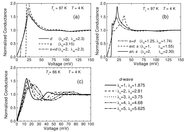
Figure 1: (a,b) Theoretical tunneling density of states for various symmetries at $T$=4 K and $\mu^{\ast}$=0. The values of $\lambda_{\mathrm{is}}$ and $\lambda_{\mathrm{an}}$ corresponding to each curve are indicated. (c) Theoretical normalized tunneling conductance in the $d$-wave symmetry, for increasing values of the coupling constants. The dip at about 2$V_{\mathrm{peak}}$ and the hump at about 3$V_{\mathrm{peak}}$ are well evident.

Figures 1(a) and 1(b) show the theoretical conductances calculated at the temperature $T=4$ K for all the symmetries analyzed here: $s$, $d$, $s+\mathrm{i}d$, $s+d$, anisotropic s and extended s. For each curve, a couple of $\lambda_{\mathrm{is}}$ and $\lambda_{\mathrm{an}}$ values is indicated which gives the expected symmetry and the correct critical temperature. As we shall see in the next section, these curves well reproduce some of the characteristic features of HTSC, such as the conductance excess below the gap and the broadening of the peak. Another apparently anomalous feature of HTSC recently reported in literature $\!{}^{{\bf?}}$ is a suppression of the conductivity at about 2$V_{\mathrm{peak}}$ (usually known as “dip”) and a subsequent enhancement at about 3$V_{\mathrm{peak}}$ (“hump”). Both these effects can be easily obtained by starting from the Eliashberg equations, using high values of the coupling constants $\!{}^{{\bf?}}$ and reducing $\omega_{\log}$ in order to maintain the critical temperature close to the experimental value. Figure 1(c) shows the conductance curves in the $d$-wave symmetry obtained for increasing values of the coupling constants. Note that the appearance of the “hump” is strictly related to the presence of the dip, as required by the conservation of the states. For instance, in the framework of the Eliashberg theory, a similar effect on the tunneling conductance curves can also be obtained by simply taking into account the finiteness of the bandwidth $\!{}^{{\bf?}}$.

The curves we have discussed so far were calculated at $T$=4 K, in view of a comparison to the experimental data which are usually obtained at the temperature of liquid helium. We also calculated the $N(V)$ curves at lower ($T$=2 K) and higher ($T$=40, 80 K) temperatures. The curves at $T$=2 K are not much different from those reported in Figures 1(a) and 1(b), apart from the fact that some fine structures (such as, for example, the first peak in the anisotropic s curve) are better distinguishable. Increasing the temperature results, in general, in a smoothing and broadening of the conductance peak at the gap edge. Above a temperature of about $T_{\mathrm{c}}/3$ all the conductances, apart the $s$-wave one, are almost the same.

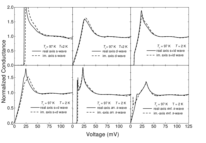
Figure 2: Comparison of the normalized tunneling conductance curves obtained by analytical continuation of the imaginary-axis solutions of the EE (dashed curves) to those obtained by direct solution of the real-axis EE (solid curves). All the curves are calculated at $T$=2 K. The agreement is good for the $d$, $s+\mathrm{i}d$ and anisotropic s symmetries. In the $s$ case, the analytical continuation shifts the gap of about 3 meV toward higher energies. In the $s+d$ case the peak of the imaginary-axis solution is lower and broader than that of the real-axis one. The extended s curves agree quite well except that for very low voltage.

Just before comparing the theoretical results to the experimental data obtained on tunnel junctions, let us discuss an important point concerning the technique here adopted for the solution of the EE. The most usual and simplest approach to the solution of these equations consists in facts in solving them in their imaginary-axis formulation, and then to continue the solutions $\Delta(\mathrm{i}\omega_{\mathrm{n}})$ and $Z(\mathrm{i}\omega_{\mathrm{n}})$ to the real axis. Actually, as we show in Figure 2, the results of this procedure only approximately agree with those obtained by directly solving the real-axis EE. Note that, in addition, the analytical continuation is meaningful only at very low temperatures (this is the reason why the curves in Figure 2 are calculated at $T$=2 K).

4 Comparison to experiments

Let us now compare the theoretical conductance curves to those obtained on optimally-doped single crystals $\!{}^{{\bf?},{\bf?}}$ of BSSCO , LSCO, YBCO, TBCO and HBCO . Here we only use for the comparison the theoretical curves obtained in the $d$ symmetry, which in fact better agree with experimental data. For each of these materials we use for $\alpha^{2}_{\mathrm{is}}F(\Omega)$ the phonon spectral density determined by neutron scattering $\!{}^{{\bf?}}$, suitably scaled to obtain the best fit. As anticipated in a previous section, a large zero-bias often appears in the experimental tunneling curves. To best fit them, we add in the EE a term taking into account the scattering from impurities $\!{}^{{\bf?}}$. We then solve the real-axis EE with varying $\lambda_{is}$ and $\lambda_{an}$, and choose the couple of values which give the best-fit curve.

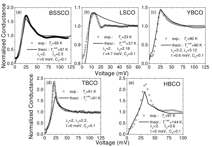
Figure 3: Comparison of the theoretical normalized tunneling conductance curves for the $s+\mathrm{i}d$-wave symmetry to those experimentally obtained on BSSCO (a), LSCO (b), YBCO (c), TBCO (d), HBCO (e). In each case the experimental and the calculated critical temperatures ($T_{\mathrm{c}}$ and $T_{\mathrm{c}}^{\mathrm{calc}}$) are indicated. Here $\Gamma$ is proportional to the impurity concentration and $C_{0}=\cot(\delta_{0})$, where $\delta_{0}$ is the scattering phase shift.

The results are shown in Figure 3 (a)-(e). In the case of BSSCO (a) and YBCO (c) the theoretical curves well agree with the experimental data, and also the calculated critical temperature is close to the measured one ($T_{\mathrm{c}}$). In the case of LSCO (b) the observed dip above the gap cannot be reproduced in the framework of Eliashberg theory. In fact, the only way for obtaining the great zero-bias value (about 0.8) which appears in this dataset, is to increase the impurity concentration to such a large amount that the peak is broadened and the dip cancels out. For TBCO (d) and HBCO (e), the height of the peak at the gap edge is quite different in the experimental and theoretical curves. Actually, this arises from the choice of the normalization for the experimental data we took from the literature. With this normalization, in fact, the experimental curves seem to violate the conservation of the states, which is instead necessarily obeyed by the theoretical curves. In these cases, the agreement has to be evaluated by comparing only the shape of the curves, as they were plotted on different scales. Finally, while for TBCO the experimental and the theoretical critical temperatures coincide, in the case of HBCO we have $T_{\mathrm{c}}^{\mathrm{calc}}$=144 K, which is much greater than the experimental one ($T_{\mathrm{c}}$=97 K)

5 Conclusions

We discussed the effect of different possible symmetries of the order parameter on the tunneling conductance curves of HTSC in the framework of the Eliashberg theory. We showed that this theory allows to explain many characteristic features of HTSC which differ from a classic BCS behaviour, and is therefore a useful tool to investigate the properties of these materials. We also tested the theoretical expectations by comparison with experimental data obtained on many different copper-oxide superconductors, and we found in many cases a reasonable agreement between the results of calculation and measurements. The most probable symmetry of the order parameter seems to be the $d$-wave, even though the sensitivity of this method in distinguish between different possible symmetries of the pairing state is strongly limited by the quality of the crystals.

References

- [1] D.J. Van Harlingen, Rev. Mod. Phys. 67 (1995) 515.
- [2] G.M. Eliashberg, Sov. Phys. JETP 3 (1963) 696.
- [3] G.A. Ummarino and R.S. Gonnelli, Physica C 328 (1999) 189.
- [4] G.A. Ummarino et al., to be published; G. A. Ummarino et al., Physica C, Proceedings of M2S-HTSC VI, Houston (U.S.) 2000 (cond-mat 9912432).
- [5] C.T. Rieck et al., Phys. Rev. B 41 (1989) 7289; G. Strinati and U. Fano, Journal of Mathematical Physics, 17 (1976) 434.
- [6] R.S. Gonnelli et al.,Physica C 275 (1997) 162.
- [7] J.F. Zasadzinski et al., Physica C Proceedings of M2S-HTSC VI, Houston (U.S.) 2000
- [8] G. Varelogiannis, Physica C 249, 87 (1995).
- [9] G. A. Ummarino and R. S. Gonnelli, Physica C Proceedings of M2S-HTSC VI, Houston (U.S.) 2000 (cond-mat 9912433).
- [10] T. Ekino et al., Physica C 263, 1920 (1996); A. M. Cucolo et al., Phys. Rev. Lett. 76, 7810 (1990); Lutfi Ozyuzer et al., Phys. Rev. B 57, 3245 (1998); J. Y. T. Wei et al., Phys. Rev. B 57, 3650 (1998).
- [11] M. Arai et al., Physica C 235-240, 1253 (1994); W. Reichardt et. al., Physica B 156-157, 897 (1989); S.L. Chaplot et al., Physica B 174, 378 (1991); Prafulla K. Jha, Sankar P. Sanyal, Physica C 271, 6 (1996).