Isotropic Conductivity of Two-Dimensional
Three-Component Symmetric Composites

Abstract

The effective dc-conductivity problem of isotropic, two-dimensional (2D), three-component, symmetric, regular composites is considered. A simple cubic equation with one free parameter for $\sigma_{e}(\sigma_{1},\sigma_{2},\sigma_{3})$ is suggested whose solutions automatically have all the exactly known properties of that function. Numerical calculations on four different symmetric, isotropic, 2D, three-component, regular structures show a non-universal behavior of $\sigma_{e}(\sigma_{1},\sigma_{2},\sigma_{3})$ with an essential dependence on micro-structural details, in contrast with the analogous two-component problem. The applicability of the cubic equation to these structures is discussed. An extension of that equation to the description of other types of 2D three-component structures is suggested, including the case of random structures.

Pacs: 72.15.Eb, 72.80.Tm, 61.50.Ah

Abstract

I Introduction

The classical duality transformation of two-dimensional (2D) heterogeneous composites, discovered by Keller [1] and independently by Dykhne [2], has been applied in a restricted set of physical contexts. The dual symmetry is based upon the observation that any 2D divergence-free field, when rotated locally at each point by $90^{o}$, becomes curl-free, and vice versa. This leads to the result that static effective physical properties of 2D infinite heterogeneous composites, like electric conductivity ${\widehat{\sigma}_{e}}$, thermal conductivity, dielectric permittivity, as well as some other static properties, satisfy some exact relationships which follow from the similarity between dual problems. For example, in the case of a two-component composite, a universal square-root law behavior of the bulk effective transport characteristics was demonstrated [2],[3]. It is also known that this transformation leads to exact results in 2D infinite composites made of an arbitrary number of components. Dykhne [2] gave sufficient conditions that, when satisfied by the component conductivities $\sigma_{i}$, lead to exact results for the isotropic bulk effective conductivity $\sigma_{e}(\sigma_{i})$. We know of only one attempt [4] to consider a 3-component 2D composite with a doubly periodic arrangement of two kinds of circular inclusions embedded into the matrix. The effective permittivity was obtained using the dipole approximation for the inclusion polarizations. But we do not know any rigorous results obtained for any 2D composite microstructure, made of 3 (or more) components, with arbitrary component conductivities. Apparently, this is not an accident but reflects the disappearance of commutativity in symmetric groups when we upgrade from the $S_{2}$ permutation group to the $S_{n}$ permutation group.

In this paper we consider the effective isotropic conductivity problem for $3$-component 2D infinite composites with translational order, with a microstructure that is symmetric in the 3 components. We formulate an approach based on the conjecture of the algebraicity of $\sigma_{e}(\sigma_{1},\sigma_{2},\sigma_{3})$ and its general properties. We have found that the algebraic equation of minimal order where all these properties can be satisfied is a cubic equation, which contains 1 free parameter, with coefficients made of the independent invariants of $S_{3}$. This equation is in agreement with Dykhne’ result (see Eq. (7)). Its predictions are compared with numerical solutions for $\sigma_{e}$ in some regular 3-component microstructures. It is also extended so as to apply to other types of 3-component composites, including random microstructures.

II TWO-DIMENSIONAL THREE-COLOR COMPOSITES

The effective dc-conductivity problem for $n$-component symmetric, 2D, infinite composites with translational order, can be reformulated with the help of n-color plane groups.

Color groups are generalizations of the classical crystallographic groups. Different colors may correspond, for example, to different chemical species or, more generally, to different values of a physical property which is defined as a tensor of $k$-rank : scalar - density $\rho$ , vector - magnetic spin m , tensor of 2-nd rank - conductivity ${\widehat{\sigma}}_{ij}$, tensor of 3-rank - piezoelectric modulus ${\widehat{d}}_{ijn}$, etc.

Every $n$-color plane group has its origin in one of the $N_{1}=$17 regular (color-blind ) plane groups. The number $N_{n}$ of n-color plane groups is a non-monotonic function of $n$: $N_{2}=46$ [5]; $N_{3}=23$; $N_{4}=96$; $N_{5}=14$; $N_{6}=90$ [6], [7]. The plane groups $n\leq 60$ are tabulated in [8].

Only 10 of the 23 3-color plane groups have a 3-fold rotation axis:

5 lattice equivalent groups - ${\sf P3(L)|P1(L)}$, ${\sf P6(L)|P2(L)}$, ${\sf P31m(L)|Cm(L)}$, ${\sf P3m1(L)|Cm(L)}$, ${\sf P6mm(L)|Cmm(L)}$ and 5 class equivalent groups - ${\sf P3(L)|P3(L^{{}^{\prime}})}$, ${\sf P6(L)|P6(L^{{}^{\prime}})}$, ${\sf P31m(L)|P3m1(L^{{}^{\prime}})}$,${\sf P3m1(L)|P31m(L^{{}^{\prime}})}$, ${\sf P6mm(L)|P6mm(L^{{}^{\prime}})}$ where ${\sf L^{{}^{\prime}}}$ is a possible sub-lattice of ${\sf L}$ invariant under rotations of order 3 [7]. All these groups are compatible only with hexagonal Bravais lattices. The 3-fold rotational symmetry makes the effective conductivity in structures governed by those groups isotropic. This follows from the Hermann theorem [9] about $k$-rank tensors in media with an inner symmetry which includes a rotation axis of highest order $r,\;r>k$. Despite their different geometries, all these structures have one important property in common: They are all invariant under the full permutation group $S_{3}$ which exchanges the colors, therefore they are related to the permutational crystallographic color groups [10].

III EFFECTIVE CONDUCTIVITY $\sigma_{e}(\sigma_{1},\sigma_{2},\sigma_{3})$ and ITS ALGEBRAIC PROPERTIES

A direct way to solve the dc-conductivity problem for an $n$-component composite begins with the local field equations

$$\nabla\times\;{\bf E}({\bf r})=0\;,\;\;\;\nabla\cdot\;{\bf J}({\bf r})=0\;,\;\;{\bf J}({\bf r})=\sigma({\bf r})\;{\bf E}({\bf r})\;,$$ (1)

along with appropriate boundary conditions for the electrical potential. The local conductivity $\sigma({\bf r})$ is a discontinuous function $\sigma({\bf r})=\sigma_{i}$, if ${\bf r}\in\Delta_{i}\;,\;i=1,2,3$ where $\Delta_{i}$ is a homogeneous part of the composite with constant conductivity $\sigma_{i}$. The isotropic effective conductivity $\sigma_{e}$ can be defined via Ohm’s law for the current ${\bf J}_{e}$ and the field ${\bf E}_{e}$ averaged over the system

$${\bf J}_{e}=\sigma_{e}\;{\bf E}_{e}\;,\;{\bf J}_{e}=\frac{1}{S}\int{\bf J}({\bf r})dS\;,\;{\bf E}_{e}=\frac{1}{S}\int{\bf E}({\bf r})dS\;.$$ (2)

Except for a medium with trivial 1D inhomogeneities (a layered medium) an exact solution of this problem does not exist for any regular or random structure. At the same time the function $\sigma_{e}(\sigma_{i})$ must have the following general properties which we are going to exploit:

${\sf 1.\;Homogeneity\;of\;1-st\;order}$

$$\sigma_{e}(k\;\sigma_{1},\;k\;\sigma_{2},\;k\;\sigma_{3})=k\;\sigma_{e}(\sigma_{1},\;\sigma_{2},\;\sigma_{3})\;.$$ (3)

This follows from the linearity of the static Maxwell equations (1) and from the definitions of the average current and field (2).

${\sf 2.\;Permutation\;invariance}$

$$\sigma_{e}({\widehat{\cal P}_{l}}\;\{\sigma_{1},\;\sigma_{2},\;\sigma_{3}\})=\;\sigma_{e}(\sigma_{1},\;\sigma_{2},\;\sigma_{3})\;.$$ (4)

where ${\widehat{\cal P}_{l}},\;l=1,...,6$ is a permutation operator of the indices $\{1,2,3\}$ (or of 3 colors). The six operators ${\widehat{\cal P}_{l}}$ form the non-commutative group $S_{3}$. The existence of permutation invariance presumes that the 3 components are distributed with equal volume fractions $p_{1}=p_{2}=p_{3}=1/3$.

${\sf 3.\;Duality}$

$$\sigma_{e}(\sigma_{1},\;\sigma_{2},\;\sigma_{3})\times\sigma_{e}(\frac{1}{\sigma_{1}},\;\frac{1}{\sigma_{2}},\;\frac{1}{\sigma_{3}})=1\;.$$ (5)

See Eq. (A16).

${\sf 4.\;Compatibility}$

$$\sigma_{e}(\sigma,\;\sigma,\;\sigma)=\sigma\;.$$ (6)

The last formula does not follow from the previous ones but reflects a natural requirement.

Dykhne [2] proved a theorem for a symmetric composite of 3 components, namely

$$\sigma_{e}(\sigma_{1},\;\sigma_{2},\;\sigma_{3})=\sqrt{\sigma_{1}\sigma_{2}}\;,\;\;\;\mbox{if}\;\;\;\sigma_{3}^{2}=\sigma_{1}\sigma_{2}\;.$$ (7)

The last formula represents the only known rigorous result for 3-color 2D isotropic composites. It can easily be shown to follow from (4) and (5). Let us mention one more conclusion which follows from (7)

$$\sigma_{e}(\sigma,\;0,\;0)=0\;,$$ (8)

which reflects the percolation property of such a composite. In fact, it is easy to construct 3-color 2D isotropic composites with the more specialized property

$$\sigma_{e}(\sigma_{1},\;\sigma_{2},\;0)=0\;.$$ (9)

Fig.1d illustrates such a structure with traps, i.e. a network of closed, simply connected loops, which enclose plaquettes of the two other colors. If any color denotes an insulator, then the effective conductivity of the composite is clearly zero. The 2-color 2D square checkerboard has a similar property. It differs from the case of Fig.1d by the value of the percolation threshold. The previous example (9) shows a non-universal behavior of $\sigma_{e}(\sigma_{i})$ even for symmetric isotropic microstructures, with essential dependence on micro-structural details, in contrast to the 2-color 2D symmetric isotropic composites, where $\sigma_{e}=\sqrt{\sigma_{1}\sigma_{2}}$ always [2].

We will look for $\sigma_{e}(\sigma_{1},\sigma_{2},\sigma_{3})$ satisfying the requirements (3 - 6) among algebraic functions. This choice is inspired by the fact that the symmetric 2-color 2D isotropic composite generates a quadratic equation for $\sigma_{e}(\sigma_{1},\sigma_{2})$. Another motivation is the situation which exists vis-a-vis some discrete 2D models in statistical mechanics, where a duality transformation exists that is similar to the one invoked here. Such a transformation exists for the Ising and Potts models [11], where the critical point equations are algebraic — quadratic equation for the Ising model on a self-dual square lattice and cubic equations for the Potts model on the mutually dual triangle and honeycomb lattices.

According to the “fundamental theorem of symmetric functions” [12] the symmetric group $S_{3}$ has 3 algebraically independent homogeneous invariants (basic invariants)

$$I_{1} = \sigma_{1}+\sigma_{2}+\sigma_{3}\;,\;I_{2}=\sigma_{1}\sigma_{2}+\sigma_{2}\sigma_{3}+\sigma_{3}\sigma_{1}\;,\;$$ (10)

$$I_{3} = \sigma_{1}\sigma_{2}\sigma_{3}\;,$$ (11)

which satisfy the obvious restrictions

$\displaystyle\frac{1}{3}I_{1}\;\geq\;\frac{I_{2}}{I_{1}}\;\geq\;3\;\frac{I_{3}}{I_{2}}\;\;,\;\;\;\frac{1}{3}I_{1}\;\geq\;\sqrt[3]{I_{3}}\;\geq\;3\;\frac{I_{3}}{I_{2}}\;,$

and can be used as independent variables instead of $\sigma_{1},\sigma_{2},\sigma_{3}$. The difference $I_{2}-I_{1}\;\sqrt[3]{I_{3}}$ can have either sign. The function $\sigma_{e}(I_{1},I_{2},I_{3})$ now satisfies (4) automatically.

It can be shown that the algebraic equation of minimal order for the function $\sigma_{e}(I_{1},I_{2},I_{3})$, which satisfies all basic requirements, is a cubic equation of the form

$$\sigma_{e}^{3}+A\;I_{1}\;\sigma_{e}^{2}-A\;I_{2}\;\sigma_{e}-I_{3}=0\;,$$ (12)

where $A$ is a free parameter responsible for the non-universality, and $\sigma_{e}$ is a value bounded from both above and below [13]

$$\frac{1}{3}I_{1}\geq\sigma_{e}\geq 3\;\frac{I_{3}}{I_{2}}\;.$$ (13)

It is easy to show that the equation (12) satisfies all basic requirements (3-6) and automatically satisfies Dykhne’s theorem (7) independently of $A$. Indeed, the requirements (3, 4, 6) one can check immediately. The duality property (5) follows when we notice that (12) is equivalent to the cubic equation for $\frac{1}{\sigma_{e}}(\frac{1}{\sigma_{1}},\;\frac{1}{\sigma_{2}},\;\frac{1}{\sigma_{3}})$:

$$\frac{1}{\sigma_{e}^{3}}+ A \;(\frac{1}{\sigma_{1}}+\frac{1}{\sigma_{2}}+\frac{1}{\sigma_{3}})\cdot\frac{1}{\sigma_{e}^{2}}-$$ (14)

$$A \;(\frac{1}{\sigma_{1}\sigma_{2}}+\frac{1}{\sigma_{2}\sigma_{3}}+\frac{1}{\sigma_{3}\sigma_{1}})\cdot\frac{1}{\sigma_{e}}-\frac{1}{\sigma_{1}\sigma_{2}\sigma_{3}}=0\;.$$ (15)

The property (7) can be proven by straightforward substitution $\sigma_{3}=\sqrt{\sigma_{1}\sigma_{2}}$ into (12) .

As we will see later, $A$ reflects not only the plane group of a color tessellation but also the shape of the elementary cell. To illuminate the meaning of $A$ let us put into (12) $A=\frac{1}{3}$. After simple algebra one obtains the following equation

$$\frac{\sigma_{e}-\sigma_{1}}{\sigma_{e}+\sigma_{1}}+\frac{\sigma_{e}-\sigma_{2}}{\sigma_{e}+\sigma_{2}}+\frac{\sigma_{e}-\sigma_{3}}{\sigma_{e}+\sigma_{3}}=0\;,$$ (16)

which coincides with the Bruggeman effective medium approximation for a symmetric, 3-component, 2D composite [14].

From restrictions (13) and after straightforward manipulations, one can show that $A$ is bounded from below

$$\infty\;\geq\;A\;\geq\;0\;.$$ (17)

It is noteworthy that the lower bound ensures that (12) has only one positive root, thus avoiding the possibility of multiple physical solutions. More accurate estimation of the lower bound for $A$, using the Hashin-Shtrikman [15] exact bounds $\sigma_{HS}^{\pm}$ for isotropic conductivity $\sigma_{e}$ of 3-component 2D composite, does not change (17). Indeed, for $\sigma_{1}>\sigma_{2}>\sigma_{3}$ one has

$$\frac{1}{3}I_{1}\geq\sigma_{HS}^{+}\geq\sigma_{e}\geq\sigma_{HS}^{-}\geq 3\;\frac{I_{3}}{I_{2}}\;,$$ (18)

where

$$\sigma_{HS}^{+} = \sigma_{1}\cdot(1+\frac{4(\sigma_{2}\sigma_{3}-\sigma_{1}^{2})}{\sigma_{2}\sigma_{3}+3\sigma_{1}(\sigma_{2}+\sigma_{3})+5\sigma_{1}^{2}})\;,$$ (19)

$$\sigma_{HS}^{-} = \sigma_{3}\cdot(1+\frac{4(\sigma_{1}\sigma_{2}-\sigma_{3}^{2})}{\sigma_{1}\sigma_{2}+3\sigma_{3}(\sigma_{1}+\sigma_{2})+5\sigma_{3}^{2}})\;.$$ (20)

Due to the ambiguity of the general case, we consider the special case $\sigma_{1}>\sigma_{2}=\sigma_{3}$. Here we have

$\displaystyle\sigma_{HS}^{+}=\sigma_{1}\cdot\frac{5+r}{1+5r}\;,\\ \sigma_{HS}^{-}=\sigma_{3}\cdot\frac{1+2r}{2+r}\;,\;\;r=\frac{\sigma_{1}}{\sigma_{3}}\geq 1\;.$

We can then derive the following lower bounds from (12), (13)

$$A>-\frac{1+5r}{1+2r}\cdot\frac{1+r}{(2+r)^{2}}\;,$$ (21)

$$A>-\frac{r}{1+5r}\cdot\frac{2+r}{1+r}\cdot\frac{1+18r+r^{2}}{1+16r+r^{2}}\;.$$ (22)

Since the last inequalities must fit all cases including $r\rightarrow\infty$, we return to (17).

IV EFFECTIVE CONDUCTIVITY of REGULAR STRUCTURES: NUMERICAL RESULTS

In the present section we will study numerically four different infinite 2D 3-color class equivalent regular structures of ${\sf P6mm(L)|P6mm(L^{{}^{\prime}})}$ and ${\sf P6(L)|P6(L^{{}^{\prime}})}$ types. In order to avoid cumbersome notations for these structures, we will use the following symbols: He (honeycomb) (Fig.1a) ; Fl (flower) (Fig.1b) ; Co (cogrose) (Fig.1c) ; Rh (rhombus) (Fig.1d).

Due to the homogeneity (3) of Eq. (12) one can rescale $\sigma_{e}(\sigma_{1},\sigma_{2},\sigma_{3})$ defining a new function $\sigma_{e}^{\prime}(\sigma_{2}^{\prime},\sigma_{3}^{\prime})$ where $\sigma_{i}^{\prime}=\sigma_{i}/\sigma_{1},\;i=e,2,3$. A typical shape of the surface defined by $\sigma_{e}^{\prime}(\sigma_{2}^{\prime},\sigma_{3}^{\prime})$ is shown in Fig. 2.

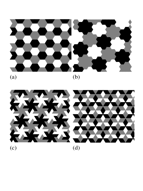
FIG. 1.: 3-color 2D composites: a) He $-{\sf G_{col}}={\sf P6mm(L)|P6mm(L^{{}^{\prime}})}$, b) Fl $-{\sf G_{col}}={\sf P6(L)|P6(L^{{}^{\prime}})}$, c) Co $-{\sf G_{col}}={\sf P6(L)|P6(L^{{}^{\prime}})}$, d) Rh $-{\sf G_{col}}={\sf P6mm(L)|P6mm(L^{{}^{\prime}})}$.

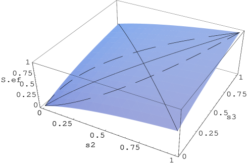
FIG. 2.: Typical shape of the surface $\sigma_{e}(\sigma_{2}^{\prime},\sigma_{3}^{\prime})$ for 3-color 2D isotropic composites. The loop where Dykhne’s theorem is satisfied is shown by the dashed lines.

This surface always contains the following points

$\displaystyle\sigma_{e}^{\prime}(0,0)=0\;,\;\;\sigma_{e}^{\prime}(1,1)=1\;,\;\;\sigma_{e}^{\prime}(\sigma,\sqrt{\sigma})=\sqrt{\sigma}\;.$

The last equality is related to the Dykhne theorem and generates a loop on the surface where (7) is satisfied. This loop is common for all such surfaces, i.e. they intersect each other on it.

We computed $\sigma_{e}^{\prime}(\sigma_{2}^{\prime},\sigma_{3}^{\prime})$ for the structures mentioned above: He, Fl, Co, Rh, and then extracted the parameter $A$ corresponding to those structures.

Before discussing these results we describe briefly the numerical algorithm which was used. This algorithm deals with hexagonal Bravais lattices represented as a grid of equilateral triangles. A subdivision procedure produces a set of $N\times N$ small similar triangles, the center of each one of them connected with the centers of 3 nearest neighboring cells by simple resistors. The resistor connecting cells $i$ and $j$ has a resistance equal to $(\sigma_{i}+\sigma_{j})/(2\sqrt{3}\sigma_{i}\sigma_{j})$, where $\sigma_{i}$ is the conductivity of the cell $i$. Translational symmetry of the composite is reflected by imposing periodic boundary conditions for the currents. The algorithm solves up to 10⁶ linear equations arising for the subdivided 3-color elementary cell. Our computational procedure always gives a sequence of effective conductivities $\sigma_{N}^{-}$, which converges monotonically (as $N\rightarrow$ 1000) from below. This fact was established by treating the solvable case following from Dykhne’s theorem, where $\sigma_{e}$ is known exactly. To get a sequence of upper bounds $\sigma_{N}^{+}$ we then used the duality property, i.e. simulating the dual problem with conductivities $1/\sigma_{2}^{\prime},\;1/\sigma_{3}^{\prime}$ and consequently obtaining a monotonic convergence from above for the sequence $\sigma_{N}^{+}$.

The simulations were done on the 4 characteristic curves on the surface where it intersects with the planes:

$$1)\;\sigma_{2}^{\prime}=0.001\;,\;\;2)\;\sigma_{2}^{\prime}=1\;,\;\;3)\;\sigma_{2}^{\prime}=\sigma_{3}^{\prime}\;,\;\;4)\;\sigma_{2}^{\prime}+\sigma_{3}^{\prime}=1\;.$$ (23)

These curves reflect the behavior of the surface relatively well in accordance with the chosen type of composite. From the assumption of the algebraic nature (12) of those curves we were able to extract, for every type of composite, a corresponding parameter $A$ by the following procedure. In a wide range of $A$, for each calculated point ($\sigma_{i}^{\prime},\;i=2,3$) on the plane, relative deviations $\epsilon$ were calculated

$$\epsilon(A,\sigma_{i}^{\prime})=\left\{\begin{array}[c]{ccl}\frac{\sigma_{e}(A,\sigma_{i}^{\prime})-\sigma_{N}^{+}}{\sigma_{e}(A,\sigma_{i}^{\prime})}&{\rm if}&\sigma_{N}^{+}<\sigma_{e}(A,\sigma_{i}^{\prime})\\ 0&{\rm if}&\sigma_{N}^{-}<\sigma_{e}(A,\sigma_{i}^{\prime})<\sigma_{N}^{+}\\ \frac{\sigma_{N}^{-}-\sigma_{e}(A,\sigma_{i}^{\prime})}{\sigma_{e}(A,\sigma_{i}^{\prime})}&{\rm if}&\sigma_{e}(A,\sigma_{i}^{\prime})<\sigma_{N}^{-}\end{array}\right.$$ (24)

and a maximal value of those deviations $\epsilon_{max}(A)$ was determined for every value of $A$ by scanning over the entire area 0$<\sigma_{2,3}^{\prime}<$1 . We then determined the best value of $A$ by minimizing the function $\epsilon_{max}(A)$. As shown in Fig. 3, $A$ for the He and Fl structures is determined by very sharp minima. The other two minima are not as sharp.

FIG. 3.: The fitting curves $\epsilon_{max}(A)$ for 4 different structures. The best value of $A$ is determined by the minimum in each curve. Those values are: He - $A_{He}=11.37,\;\epsilon_{max}^{He}$=.00026 ; Fl - $A_{Fl}=3.76,\;\epsilon_{max}^{Fl}$=.001 ; Co - $A_{Co}=.305,\;\epsilon_{max}^{Co}$=.022 ; Rh - $A_{Rh}=0,\;\epsilon_{max}^{Rh}$=.065.

As one could expect, the Rh structure has $A=0$ since this is the unique value of $A$ for which the solution of equation (12) has the features typical of the structures with traps. The values of $A$ which minimize $\epsilon_{max}(A)$ for the other structures are listed in the caption of Fig. 3.

Figs. 4–7 show the computed results for upper and lower bounds on the relative bulk effective conductivity $\sigma_{e}^{\prime}$, i.e. $\sigma_{N}^{+}(\sigma_{2}^{\prime},\sigma_{3}^{\prime})$ and $\sigma_{N}^{-}(\sigma_{2}^{\prime},\sigma_{3}^{\prime})$ at maximal $N$, for the 4 microstructures of Fig. 1. Note that these upper and lower bounds often appear to coincide due to insufficient resolution in the figures. The axes in the figures are labeled with S.ef for the relative bulk effective conductivity $\sigma_{e}^{\prime}$ and s1, s2, s3 for the component relative conductivities $\sigma_{1}^{\prime}=1,\sigma_{2}^{\prime},\sigma_{3}^{\prime}$ respectively.

The pairs of almost merged points shown in Fig. 7 correspond to barely separated upper and lower bounds.

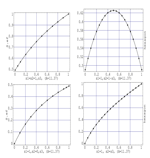
FIG. 4.: Numerical results $\sigma_{N}^{+}(\sigma_{2}^{\prime},\sigma_{3}^{\prime}),\;\sigma_{N}^{-}(\sigma_{2}^{\prime},\sigma_{3}^{\prime})$ (black dots) and analytic solution $\sigma_{e}^{\prime}(\sigma_{2}^{\prime},\sigma_{3}^{\prime})$ of cubic equation (12) with $A$=11.37 (bold line) at the four sections (23) of the surface corresponding to the He - structure.

FIG. 5.: Numerical results $\sigma_{N}^{+}(\sigma_{2}^{\prime},\sigma_{3}^{\prime}),\;\sigma_{N}^{-}(\sigma_{2}^{\prime},\sigma_{3}^{\prime})$ (black dots) and analytic solution $\sigma_{e}^{\prime}(\sigma_{2}^{\prime},\sigma_{3}^{\prime})$ of cubic equation (12) with $A$=3.76 (bold line) at the four sections (23) of the surface corresponding to the Fl - structure.

FIG. 6.: Numerical results $\sigma_{N}^{+}(\sigma_{2}^{\prime},\sigma_{3}^{\prime}),\;\sigma_{N}^{-}(\sigma_{2}^{\prime},\sigma_{3}^{\prime})$ (black dots) and analytic solution $\sigma_{e}^{\prime}(\sigma_{2}^{\prime},\sigma_{3}^{\prime})$ of cubic equation (12) with $A$=0.305 (bold line) at the four sections (23) of the surface corresponding to the Co - structure.

FIG. 7.: Numerical results $\sigma_{N}^{+}(\sigma_{2}^{\prime},\sigma_{3}^{\prime}),\;\sigma_{N}^{-}(\sigma_{2}^{\prime},\sigma_{3}^{\prime})$ (black dots) and analytic solution $\sigma_{e}^{\prime}(\sigma_{2}^{\prime},\sigma_{3}^{\prime})$ of cubic equation (12) with $A$=0 (bold line) at the three sections (23) of the surface corresponding to the Rh - structure. The fourth dependence $\sigma_{e}^{\prime}(0,\sigma_{3}^{\prime})=$0 is omitted because of its triviality.

V EFFECTIVE CONDUCTIVITY OF RANDOM STRUCTURES: EXTENSION OF THE ALGEBRAICITY CONJECTURE

In this chapter we discuss briefly a possible extension of the algebraicity conjecture for 2D three-component structures, which are non-regular but macroscopically homogeneous. On length scales large compared to the inhomogeneities, we can characterize the macroscopic response of such a medium by a single number, the plane effective conductivity $\sigma_{e}$. A reexamination of the basic properties (3-6) of $\sigma_{e}(\sigma_{1},\sigma_{2},\sigma_{3})$ shows that one of them (4) must be discarded, while the other three (homogeneity of 1-st order, duality, and compatibility) continue to be valid. It is important to note that these properties hold irrespective of whether the microstructure of the (isotropic) composite is ordered or disordered.

Instead of Eq. (4), which implies full symmetry under the group $S_{3}$ of all 3-color permutations, we first consider the case where the structure is only symmetric under the group $C_{3}$ of cyclic 3-color permutations: 1 $\rightarrow$ 2 $\rightarrow$ 3 $\rightarrow$ 1. An example of such a microstructure is shown in Fig. 8. (Note the arrangement of “flowers” near the center of that figure.) It follows that $\sigma_{e}(\sigma_{1},\sigma_{2},\sigma_{3})$ is a cyclic permutation invariant function. The group $C_{3}$ is a subgroup of index 2 of the full permutation group $S_{3}$, which characterizes all the regular structures He, Fl, Co, Rh discussed in the previous sections.

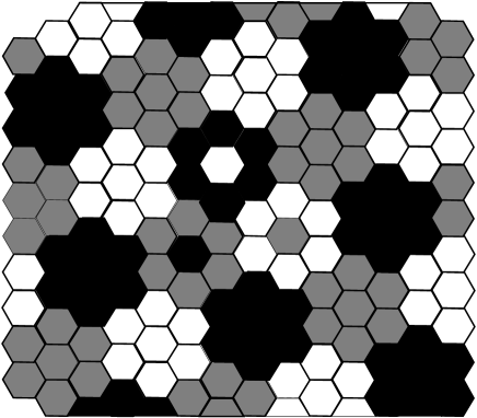
FIG. 8.: 3-color 2D composite of Fl structure locally disturbed in the centers of only three plaquettes with different colors. Such color tessellation preserves an equal fraction of every color and is invariant under the cyclic permutation group $C_{3}$, but not under the full $S_{3}$ permutation group.

Being non-reflecting, the group $C_{3}$ has more basic invariants than the group $S_{3}$ [see Eq. (11)], namely [12]

$$I_{1}(C_{3}) = \sigma_{1}+\sigma_{2}+\sigma_{3}\;,\;\;I_{2}(C_{3})=\sigma_{1}\sigma_{2}+\sigma_{2}\sigma_{3}+\sigma_{3}\sigma_{1}\;,$$ (25)

$$I_{3}(C_{3}) = \sigma_{1}\sigma_{2}\sigma_{3}\;,\;I_{4}(C_{3})=(\sigma_{1}-\sigma_{2})(\sigma_{2}-\sigma_{3})(\sigma_{3}-\sigma_{1})\;.$$ (26)

Nevertheless, the additional cubic invariant $I_{4}(C_{3})$ cannot be incorporated into a cubic equation for $\sigma_{e}$, because that would violate the duality requirement. Thus, we are lead back to the cubic equation (12), which is dictated not only by the strong requirement (4) of the full permutation invariance $S_{3}$, but even by the milder requirement of cyclic permutation invariance $C_{3}$.

In the case of a random composite, we usually characterize the microstructure by a statistical distribution function of the local conductivity, which can be either $\sigma_{1}$, $\sigma_{2}$, or $\sigma_{3}$ at any point. Such a description results in an ensemble of representative structures, each one with its own form for the function $\sigma_{e}(\sigma_{1},\sigma_{2},\sigma_{3})$. If we assume that the distribution function has the permutation symmetry of either $S_{3}$ or $C_{3}$, then the ensemble average of $\sigma_{e}(\sigma_{1},\sigma_{2},\sigma_{3})$ will have that symmetry too, even though individual samples may violate it. It follows that, the same considerations which led us to stipulate the form (12), for the minimal polynomial equation that $\sigma_{e}$ could satisfy for regular structures, also lead to that same equation for random structures, if the statistical model for those structures is invariant under either $S_{3}$ or $C_{3}$. Numerical tests of this conjecture remain to be performed.

VI CONCLUSION

In the present paper we have introduced the algebraicity conjecture for the effective conductivity problem of isotropic 2D three-component regular composites. This conjecture is based on the general properties which are satisfied by the effective conductivity $\sigma_{e}(\sigma_{1},\sigma_{2},\sigma_{3})$. The algebraic equation of minimal order for $\sigma_{e}$ is a cubic equation with 1 positive free parameter $A$ responsible for the non-universality. This equation satisfies Dykhne’s theorem (7) independently of $A$ and has only one positive root, thus avoiding the possibility of multiple physical solutions. The value $A=1/3$ corresponds exactly to the Bruggeman effective medium approximation for a 2D composite with 3 equally partitioned components.

We have found support for this conjecture by numerical calculations on four different infinite 2D 3-color class equivalent regular structures of ${\sf P6mm(L)|P6mm(L^{{}^{\prime}})}$ and ${\sf P6(L)|P6(L^{{}^{\prime}})}$ types: He, Fl, Co, Rh. We have established that $\sigma_{e}(\sigma_{1},\sigma_{2},\sigma_{3})$ is a non-universal function with essential dependence on the microstructure even for totally symmetric structures:

1) The cubic equation (12) with $A$=11.37 governs the conductivity problem in He structure with a very high precision $\epsilon_{max}\simeq 10^{-4}$.

2) There is good agreement ($\epsilon_{max}\simeq 10^{-3}$) between the cubic equation with $A$=3.76 and numerical results for the Fl structure.

3) In the Co structure the estimated value $A$=.305 is near $1/3$, which would follow from the Bruggeman effective medium approximation. This may indicate some similarity between the conducting properties of a 3-component random microstructure and those of the ordered Co structure.

4) The Rh structure needs special attention. It belongs to the family of structures with unicolor traps, i.e. with structures where the presence of just one non-conducting ($\sigma_{1}=0$) component is enough to make the composite an insulator ($\sigma_{e}=0$). In percolation theory this corresponds to a threshold $p_{3}=1/3$, in contrast with a 2-color composite where $p_{2}=1/2$. If the cubic equation is valid for this structure with $A$=0, then $\sigma_{e}=\sqrt[3]{\sigma_{1}\sigma_{2}\sigma_{3}}$. Unfortunately, these computations are unable to resolve this question for the Rh microstructure.

5) The different microstructures which belong to a common plane symmetry group (He, Rh - ${\sf P6mm(L)|P6mm(L^{{}^{\prime}})}$, Fl, Co - ${\sf P6(L)|P6(L^{{}^{\prime}})}$) are characterized by distinct values of $A$. This means that this parameter has a topological nature and is sensitive to more than just the symmetry properties of the elementary cell or the plane group of the entire color lattice.

Finally we discussed a possible extension of the algebraicity conjecture to other types of 2D three-component structures. First we showed that even if the microstructure is only invariant under the $C_{3}$ subgroup of the $S_{3}$ permutation group, a cubic equation for $\sigma_{e}$ must still have the form (12). We then extended this conjecture also to the case of random microstructures, described by any statistical model that is invariant under either $S_{3}$ or $C_{3}$. To test this idea, it would be useful to do numerical calculations on such structures. This is left for future investigations.

A

We now give a simple proof of the duality relations for a 2D isotropic medium composed of an arbitrary number $n$ of isotropic components.

Suppose a 2D medium with a continuous distribution of conductivity $\sigma({\bf r})$ is subjected to an average electric field ${\bf E}_{e}$. The system of equations consists of Ohm’ law

$${\bf J}({\bf r})={\widehat{\sigma}}({\bf r})\;{\bf E}({\bf r})\;,$$ (A1)

and the equations for local fields

$$\nabla\times\;{\bf E}({\bf r})=0\;,\;\;\;\nabla\cdot\;{\bf J}({\bf r})=0\;$$ (A2)

with appropriate boundary conditions on the electrical potential.

We are interested in the relation between the current ${\bf J}_{e}$ averaged over the system, ${\bf J}_{e}=S^{-1}\int{\bf J}({\bf r})dS$ and the averaged field ${\bf E}_{e}=S^{-1}\int{\bf E}({\bf r})dS$. By virtue of the linearity of (A1, A2) this relation will also be linear

$${\bf J}_{e}={\widehat{\sigma}_{e}}\;{\bf E}_{e}\;,\;\;\;{\widehat{\sigma}}_{e}={\widehat{\sigma}}_{e}\;\{{\widehat{\sigma}}({\bf r})\}\;.$$ (A3)

where the tensor of the bulk effective conductivity ${\widehat{\sigma}}_{e}={\widehat{\sigma}}_{e}\;\{{\widehat{\sigma}}({\bf r})\}$ is actually a tensorial functional. In the case of $n$ homogeneous anisotropic components, the latter becomes a tensorial function ${\widehat{\sigma}}_{e}\;({\widehat{\sigma}}_{1},{\widehat{\sigma}}_{2},...,{\widehat{\sigma}}_{n})$. Further simplification arises when all components are isotropic — ${\widehat{\sigma}}_{e}\;(\sigma_{1},\sigma_{2},...,\sigma_{n})$ and, finally when the entire composite is also an isotropic medium — $\sigma_{e}\;(\sigma_{1},\sigma_{2},...,\sigma_{n})$.

In order to transform to the dual problem we rotate the $x,y\;$-components of ${\bf J}$ and ${\bf E}$ by $90^{o}$ in the plane

$${\bf J}^{\prime}({\bf r})={\widehat{R}}\;{\bf E}({\bf r})\;,\;\;{\bf E}^{\prime}({\bf r})={\widehat{R}}\;{\bf J}({\bf r})\;,\;\;{\bf J}^{\prime}({\bf r})={\widehat{\sigma}}^{\prime}({\bf r})\;{\bf E}^{\prime}({\bf r})\;,$$ (A4)

$${\widehat{\sigma}}^{\prime}({\bf r})={\widehat{R}}\;{\widehat{\sigma}}^{-1}({\bf r})\;{\widehat{R}}^{-1}\;,\;\;{\widehat{R}}=\left(\begin{array}[]{cc}0&-1\\ 1&0\end{array}\right).$$ (A7)

Eqs. A2 are thereby transformed as follows

$\displaystyle\nabla\cdot\;{\bf J}^{\prime}({\bf r})=\nabla\times\;{\bf E}({\bf r})=0\;,\;\;\nabla\times\;{\bf E}^{\prime}({\bf r})=\nabla\cdot\;{\bf J}({\bf r})=0\;,$

while ${\bf J}_{e}^{\prime}$ and ${\bf E}_{e}^{\prime}$ are connected by

$${\bf J}^{\prime}_{e}={\widehat{\sigma}}^{\prime}_{e}\;{\bf E}^{\prime}_{e}\;,\;\;{\widehat{\sigma}}^{\prime}_{e}={\widehat{R}}\;{\widehat{\sigma}}_{e}^{-1}{\widehat{R}}^{-1}\;,$$ (A8)

where the bulk effective conductivity tensor of the dual problem ${\widehat{\sigma}}^{\prime}_{e}$ is defined in accordance with (A3)

$${\widehat{\sigma}}^{\prime}_{e}={\widehat{\sigma}}_{e}\{{\widehat{\sigma}}^{\prime}({\bf r})\}={\widehat{\sigma}}_{e}\;\{{\widehat{R}}\;{\widehat{\sigma}}^{-1}({\bf r}){\widehat{R}}^{-1}\}\;.$$ (A9)

The last two equations (A8,A9) give a duality relation

$${\widehat{\sigma}}_{e}\;\{{\widehat{R}}\;{\widehat{\sigma}}^{-1}({\bf r}){\widehat{R}}^{-1}\}\cdot{\widehat{R}}\cdot{\widehat{\sigma}}_{e}\;\{{\widehat{\sigma}}({\bf r})\}\cdot{\widehat{R}}^{-1}={\widehat{I}}\;,$$ (A10)

where ${\widehat{I}}$ is the unit matrix. If, instead of the continuous fields $\sigma({\bf r})$ we deal with anisotropic media composed of $n$ homogeneous anisotropic components, then

$${\widehat{\sigma}}_{e}\;({\widehat{R}}\;{\widehat{\sigma}}^{-1}_{1}\;{\widehat{R}}^{-1},{\widehat{R}}\;{\widehat{\sigma}}^{-1}_{2}\;{\widehat{R}}^{-1},...,{\widehat{R}}\;{\widehat{\sigma}}^{-1}_{n}\;{\widehat{R}}^{-1})\cdot{\widehat{R}}\cdot$$ (A11)

$$\cdot{\widehat{\sigma}}_{e}\;({\widehat{\sigma}}_{1},{\widehat{\sigma}}_{2},...,{\widehat{\sigma}}_{n})\cdot{\widehat{R}}^{-1}={\widehat{I}}\;.$$ (A12)

In the case of an anisotropic composite with $n$ homogeneous isotropic components we will have

$${\widehat{\sigma}}_{e}\;(\sigma^{-1}_{1},\sigma^{-1}_{2},...,\sigma^{-1}_{n})\cdot{\widehat{R}}\cdot{\widehat{\sigma}}_{e}\;(\sigma_{1},\sigma_{2},...,\sigma_{n})\cdot{\widehat{R}}^{-1}={\widehat{I}}\;.$$ (A13)

The principal values of ${\widehat{\sigma}}_{e}$ satisfy Keller’s theorem

$${\widehat{\sigma}}_{e}^{xx}(\sigma^{-1}_{1},\sigma^{-1}_{2},...,\sigma^{-1}_{n})\cdot{\widehat{\sigma}}_{e}^{yy}(\sigma_{1},\sigma_{2},...,\sigma_{n})=1\;,$$ (A14)

$${\widehat{\sigma}}_{e}^{yy}(\sigma^{-1}_{1},\sigma^{-1}_{2},...,\sigma^{-1}_{n})\cdot{\widehat{\sigma}}_{e}^{xx}(\sigma_{1},\sigma_{2},...,\sigma_{n})=1\;.$$ (A15)

In general, the directions of the principal axes depend on the values of $\sigma_{1},\sigma_{2},$ etc. But when the symmetry of the microstructure is sufficiently high, those directions will be fixed by that symmetry. Finally, in the case of an isotropic composite, the last equations reduce to the self-duality relation

$$\sigma_{e}(\sigma^{-1}_{1},\sigma^{-1}_{2},...,\sigma^{-1}_{n})\cdot\sigma_{e}(\sigma_{1},\sigma_{2},...,\sigma_{n})=1\;.$$ (A16)

REFERENCES

• [1] J. B. Keller, J. Math. Phys. 5, 548 (1964)
• [2] A. M. Dykhne, Zh. Eksp. Teor. Fiz. 59, 110 (1970) [Sov. Phys. JETP 32, 63 (1970)]
• [3] K. S. Mendelson, J. of Apl. Phys. 46, 917 (2); 4740 (11) (1975)
• [4] Yu. P. Emets, Zh. Eksp. Teor. Fiz. 114, 1121 (1998) [Sov. Phys. JETP 87, 612 (1998)]
• [5] N. V. Belov, Kristallografia, 1, 621 (1956);  N. V. Belov and E. N. Belova, Kristallografia, 2, 21 (1957)
• [6] M. Senechal, Zs. Kristallogr. 142, 1 (1975); Discrete Appl. Math. 1, 51 (1979)
• [7] J. D. Jarratt and R. L. E. Schwarzenberger, Acta Crystallogr. A 36, 884 (1980)
• [8] T. W. Wieting, The mathematical theory of chromatic plane ornaments, New York, Marcel Dekker,  (1982)
• [9] C. Hermann, Zs. Kristallogr. 89, 32 (1934)
• [10] D. B. Litwin, J. N. Kotzev and J. L. Birman, Phys. Rev. B 26, 6947 (1982)
• [11] R. J. Baxter, Exactly solved models in statistical mechanics, New York, Academic Press,  (1982)
• [12] P. J. Olver, Classical Invariant Theory, Cambridge, University Press, (1998)
• [13] O. Wiener, Abh. S$\ddot{a}$chs. Akad. Wiss. Leipzig Math.-Naturwiss. Kl. 32, 509, (1912)
• [14] D. A. G. Bruggeman, Ann. Physik (Leipzig) 24, 636, (1935); R. Landauer, in ”Electrical Transport and Optical Properties of Inhomogeneous Media” , Eds. J. C. Garland and D. B. Tanner, AIP Conf.Proceed. No. 40, 2, (1978)
• [15] Z. Hashin and S. Shtrikman, J. Appl. Phys. 33, 3125 (1962)
A