Direct calculation of the hard-sphere crystal/melt interfacial free energy

Abstract

We present a direct calculation by molecular-dynamics computer simulation of the crystal/melt interfacial free energy, $\gamma$, for a system of hard spheres of diameter $\sigma$. The calculation is performed by thermodynamic integration along a reversible path defined by cleaving, using specially constructed movable hard-sphere walls, separate bulk crystal and fluid systems, which are then merged to form an interface. We find the interfacial free energy to be slightly anisotropic with $\gamma$ = 0.62$\pm 0.01$, 0.64$\pm 0.01$ and 0.58$\pm 0.01k_{B}T/\sigma^{2}$ for the (100), (110) and (111) fcc crystal/fluid interfaces, respectively. These values are consistent with earlier density functional calculations and recent experiments measuring the crystal nucleation rates from colloidal fluids of polystyrene spheres that have been interpreted [Marr and Gast, Langmuir 10, 1348 (1994)] to give an estimate of $\gamma$ for the hard-sphere system of $0.55\pm 0.02k_{B}T/\sigma^{2}$, slightly lower than the directly determined value reported here.

A detailed microscopic description of the interface between a crystal and its melt is necessary for a full understanding of such important phenomena as homogeneous nucleation and crystal growth[1, 2, 3]. Computer simulation studies of model materials have had some success in elucidating the phenomenology of such systems[4], the importance of such work being enhanced by the near absence of reliable experimental studies. These efforts, however, have been primarily focused on structural and dynamical properties, since the central thermodynamic property, the crystal/melt interfacial free energy, is difficult to measure by simulation or experiment. In this work we report the results of a direct calculation via molecular-dynamics (MD) simulation of the crystal/melt surface free energy of the hard-sphere system, one of the most important reference models for simple materials.

The crystal/melt surface free energy, $\gamma$, is defined as the (reversible) work required to form a unit area of interface between a crystal and its coexisting melt. Experimentally, $\gamma$ can be measured either indirectly from measurements of crystal nucleation rates interpreted through classical nucleation theory, or directly by contact angle measurements [1]. Using the former method, Turnbull [5] estimated $\gamma$ for a number of materials and found a strong empirical correlation between the values obtained and the latent heat of fusion for each material given by the relation $\gamma\approx C_{T}\Delta_{f}H\rho^{2/3}$, where $\rho$ is the number density of the crystal and with $C_{T}$ (the Turnbull coefficient) taking on the value 0.45 for most metals and 0.32 for other mostly nonmetallic materials. For the hard-sphere system considered in this work, recent experiments[6] of the crystallization kinetics of a colloidal suspension of uncharged polystyrene spheres, which closely mimic hard spheres, have been interpreted within a classical nucleation model to yield an estimate for $\gamma$ of the hard-sphere system of 0.55$\pm 0.02$$k_{B}T/\sigma^{2}$ [7]. This value is in agreement [8] with that predicted using the empirical relationship above assuming a $C_{T}$ of 0.45 and values of $\Delta_{f}H$ and coexistence densities for hard spheres as determined by MD simulation [9]. Unfortunately, the accuracy of the values of $\gamma$ obtained from nucleation rates is severely limited by the approximations inherent in classical nucleation theory. More accurate values can be obtained directly using contact angles, but such experiments are difficult and only a few materials have been studied to date. One notable example is a series of grain boundary contact angle experiments on bismuth [10] that determined $\gamma$ to be relatively independent of crystal orientation at 61.3$\times 10^{-3}$ J/m², which is about 10% higher than Turnbull’s estimate from nucleation rates of 54.4$\times 10^{-3}$ J/m².

In recent years, the primary theoretical approach to studying the structure and thermodynamics of the crystal/melt interface has been density-functional theory (DFT) [11, 12, 13, 14, 15, 16]. For these studies, the hard-sphere system has been the benchmark calculation, due to the simplicity of the interaction and the availability of accurate, analytical formulas for the properties of the fluid. However, as discussed by Marr [8] the value of $\gamma$ obtained is highly dependent on the approximations used to construct the DFT and the reported values range from 0.25 to 4.00$k_{B}T/\sigma^{2}$. The DFT studies also disagree dramatically in the degree of orientation dependence of the interfacial free energy. Unfortunately, in the absence of simulation results it has been difficult to assess the validity of the individual approaches, although only the DFT approach of Curtin[13] ($\gamma=0.62k_{B}T/\sigma^{2}$) and the related one of Marr and Gast[7] ($\gamma=0.60k_{B}T/\sigma^{2}$) come close to the nucleation result of $0.55\pm 0.02k_{B}T/\sigma^{2}$.

To date, the only reliable calculation of the crystal/melt interfacial free energy via simulation is that of a system of particles interacting via a truncated Lennard-Jones potential by Broughton and Gilmer [17]. In that work, a series of continuous, external “cleaving” potentials are used to separate (cleave) separate samples of bulk liquid and fcc crystal, prepared at the calculated coexistence temperature and densities. The solid and liquid slabs thus produced are then placed next to one another and the cleaving potentials removed to merge them into a coexisting interface. The reversible work to perform these steps can be calculated by thermodynamic integration, giving a direct calculation of $\gamma$ for this system. The values of $\gamma$ at the triple point were found to be statistically isotropic with $\gamma\sigma^{2}/\epsilon=0.35\pm 0.02,0.34\pm 0.02$ and $0.36\pm 0.02$ for the (111), (100) and (110) interfaces, respectively.

For the hard-sphere system, the Broughton-Gilmer procedure must be modified since the algorithm for MD simulation of discontinuous hard-core potentials is conceptually very different from the algorithm for continuous potentials. The latter are performed by integrating the system of ordinary differential equations, while in the former the dynamical algorithm proceeds on a collision by collision basis. Therefore, incorporating continuous cleaving potentials into the collisional algorithm would result in lost efficiency and substantial modification of the structure of the algorithm.

In this Letter we introduce an approach, which uses only hard-sphere interactions in order to cleave the bulk hard-sphere systems. This allows us to apply the Broughton-Gilmer cleaving procedure to the hard-sphere system with only minor changes to the algorithm structure. The idea of our approach is illustrated in Fig. 1. To cleave the bulk system at a cleaving plane (shown by the dashed line in Fig. 1), the spheres are assigned types 1 or 2 based on their position relative to the plane. Next, two walls, which are also assigned types 1 and 2, are placed on the opposite sides of the cleaving plane. The two types are introduced in order to specify interaction between the spheres and the walls; namely, the walls interact only with the spheres of similar type. Therefore, when the walls are placed as shown in Fig. 1, and the distance from the walls to the cleaving plane is larger than the sphere radius, the walls do not interact with the spheres. It is important that, during a simulation run, a sphere changes its type whenever it crosses the cleaving plane. Because of the periodic boundary conditions in the $z$ direction, another plane must be defined sufficiently far away from the cleaving plane, where the spheres also change type.

The cleaving of the system is achieved by slowly moving the walls towards each other (as shown by the arrows in Fig. 1), starting from the initial position $z_{i}$, where the walls do not interact with the system, till $z_{f}$, where the spheres of different types no longer collide with each other at the cleaving plane.

FIG. 1.: Diagram illustrating the cleaving of the bulk hard-sphere system by two moving walls. Spheres are assigned types 1 and 2 based on their position with respect to the cleaving plane (dashed line). Two walls of types 1 and 2, which interact only with spheres of similar type, are placed on the opposite sides of the cleaving plane, so that initially there are no collisions between walls and spheres (as shown on the diagram). The system is then cleaved by moving the walls in directions indicated by the arrows.

During the process, the average pressure on the walls, $P(z)$, is measured as a function of wall position. The work per unit area required to perform the cleaving is given by the integral

$$w=\int^{z_{f}}_{z_{i}}P(z)\;dz\>.$$ (1)

Thus the crystal-fluid interfacial free energy, $\gamma$, can be measured in the reversible process involving the following four steps: (1) Cleave the bulk crystal by inserting two walls at the cleaving plane and moving them from $z_{i}$ to $z_{f}$; (2) Cleave the bulk fluid in a similar way; (3) Juxtapose the cleaved crystal and fluid systems by changing the periodic boundary conditions while retaining the crystal and fluid systems restricted by the respective cleaving walls; (4) Slowly move the walls back to their initial positions with respect to the cleaving planes. This series of steps is the same as that used by Broughton and Gilmer[17], except that, in our case, no work is done on the system in step 3. The interfacial free energy is given by the sum $\gamma=w_{1}+w_{2}+w_{4}\;$, where $w_{4}$ is negative and consists of the work done by the walls on the crystal and fluid parts of the system during the process of removing the cleaving walls.

The structure of the cleaving walls is crucial to the success of the procedure. The main requirement is that the insertion of the walls perturbs the systems as little as possible. Our approach is to use walls made of layers of ideal crystal oriented in correspondence with the orientation of the crystal system. For the (100) and (111) orientations it is sufficient to use one layer, while for the (110) orientation we use two layers. Such a choice of the wall structure ensures minimal perturbation of the cleaved crystal, while the cleaved fluid is expected to form properly oriented interfacial layers. On a technical side, the implementation of such a wall structure is quite simple, since we can treat collisions with the walls in the same manner we treat collisions between all the spheres in the system, except that the spheres forming the walls are assigned infinite mass.

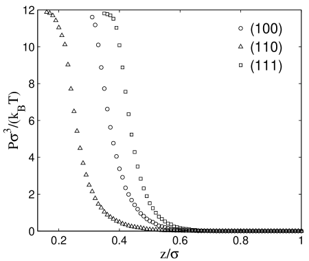
FIG. 2.: Step 1: Cleaving crystal system. Pressure on the cleaving walls as a function of wall position for the three orientations of the interface. The error bars are smaller than the size of the symbols.

The position of the walls, $z$, is measured by the distance of the centers of the spheres forming the walls to the cleaving plane. Obviously, the walls do not interact with the system when $z>\sigma$. Therefore, we set the initial position of the walls at $z_{i}=\sigma$. The pressure $P(z)$ is obtained by moving the walls from $z_{i}$ to $z_{f}$ in steps of 0.01$\sigma$. In order to move the walls to a new position, we assign a small velocity (about 0.1% of the average particle velocity) to the spheres forming the walls, and run the simulation until the walls reach the new position. At that moment the wall velocity is set to zero, and the velocities of the particles are rescaled in order to restore the initial value of the total kinetic energy of the system. Before measuring the pressure, we allow the system to relax in an equilibration run. In order to verify the reversibility of the cleaving process, we have also simulated the reverse process and measured the pressure while moving the walls from $z_{f}$ back to $z_{i}$. The details of the simulation process and obtained results follow.

Step 1: Cleaving the crystal  For each of the three orientations, we start with a crystal at a density $\rho_{c}=1.037\sigma^{-3}$, which corresponds to the crystal-fluid coexistence pressure of 11.55$k_{B}T\sigma^{-3}$[18]. In order to minimize the size effects and the amount of stress in the crystal introduced by the cleaving walls, we use large systems of about 8000 spheres and approximate dimensions of $14\sigma\times 14\sigma\times 40\sigma$. (To perform the simulations efficiently for such large systems, we use the algorithm of Rappaport [19].) The cleaving plane is placed in the middle between two crystal layers. The dependence of the pressure on the wall position is shown in Fig. 2. The walls do not interact with the crystal until they move sufficiently close to the crystal layers (about 0.7$\sigma$ for all orientations). Then the pressure on the walls quickly rises to slightly above the bulk crystal pressure. The steepness of the rise is directly related to the compactness of the layers for each orientation. The final positions, $z_{f}$, where the spheres of different types no longer collide across the cleaving plane, were determined to be 0.31$\sigma$, 0.16$\sigma$, and 0.35$\sigma$ for the (100), (110), and (111) system orientations, respectively. No hysteresis was observed in the reverse process.

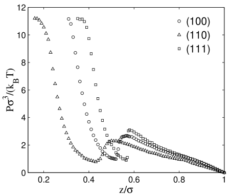
FIG. 3.: Step 2: Cleaving fluid system. Pressure on the cleaving walls as a function of wall position for the three orientations of the interface. The error bars are of the order of the size of the symbols.

Step 2: Cleaving the fluid  The fluid systems consisting of about 7400 particles are prepared at the coexistence density $\rho_{f}=0.939\sigma^{-3}$ using box dimensions nearly identical to the crystal systems. Unlike in step 1, the cleaving walls begin to interact with the fluid system as long as $z<\sigma$. As can be seen in Fig. 3, the pressure on the walls increases approximately linearly until the fluid near the cleaving walls begins to develop significant crystal-like ordering commensurate with the wall structure. At that point the pressure in the bulk fluid decreases to about 11.2$k_{B}T\sigma^{-3}$, after which the dependence of pressure on the wall position follows essentially the same curve as during the cleaving of the crystal system, which leads to the same values of $z_{f}$ as in step 1.

Simulation of the reverse process shows that the ordering of the fluid against the walls is the source of some hysteresis. However, we have found that the magnitude of the hysteresis can be always reduced to within the statistical error by increasing the duration of the equilibration run. In other words, at every position of the cleaving walls, the pressure on the walls eventually converges to the same value (within the statistical error bounds) in both forward and reverse processes.

Step 3: Changing boundary conditions  The combined system has two cleaving planes and four walls. The crystal part of the system and the two walls restraining it are assigned type 1, while the fluid part and the other two walls are assigned type 2.

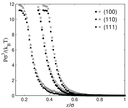
FIG. 4.: Step 4: Removing the cleaving walls. Pressure on the cleaving walls as a function of wall position for the three orientations of the interface. Filled and open symbols indicate pressure on the walls restraining fluid and crystal parts of the system, respectively. The error bars are of the order of the size of the symbols.

Step 4: Removing the cleaving walls  As can be seen in Fig. 4, the pressure on the walls restraining crystal and fluid parts of the system is essentially the same as in steps 1 and 2, respectively, except that the fluid part retains its structure in the interfacial region. Thus the main contribution to the interfacial free energy comes from the pressure of the fluid on the cleaving walls before significant crystal-like ordering at the wall develops.

The work done during each step and the resulting interfacial free energy for each of the three orientations is given in Table I. The average values of $\gamma$ for the three orientations is about 0.61$k_{B}T/\sigma^{2}$, which corresponds to a Turnbull coefficient of 0.51. This average value is about 10% higher than the value determined from nucleation rates on colloidal crystals, consistent with the differences found in other materials, such as bismuth (discussed above). Note that the hard-sphere $\gamma$ values are slightly anisotropic and increase in the order of (111), (100) and (110). That (111) has the lowest interfacial free energy is perhaps not surprising, since the (111) crystal face resembles most the structure adopted by the fluid against a structureless wall [18].

It is generally accepted that the structure and thermodynamics of dense simple fluids is dominated by the repulsive part of the potential, which can often be well approximated as a hard sphere, and the effect of the attractive part of the potential can be viewed as a small perturbation. If one considers the truncated Lennard-Jones system studied by Broughton and Gilmer and calculates an effective hard-sphere diameter at the triple point ($T=0.617\epsilon/k_{B}$), using the Barker-Henderson approach[20], one obtains a value of ($0.39\epsilon/\sigma^{2}$) simply by rescaling the hard-sphere result calculated here. Thus, the attractive part of this potential accounts for only about 10% of the total $\gamma$, which is consistent with a similar observation by Curtin on the basis of DFT calculations [13].

To summarize, we have determined the crystal/melt interfacial free energy, $\gamma$ for the hard-sphere system directly from simulation using a method that is similar to that Broughton and Gilmer [17] used for the truncated Lennard-Jones system except that we have replaced their external cleaving potentials with specially constructed cleaving walls. Although the method of cleaving walls is especially advantageous for the hard-sphere system, it could also be easily applied in modified form to continuous potentials. The hard-sphere $\gamma$ obtained is only slightly dependent upon orientation and averages about 0.61$k_{B}T/\sigma$, consistent with some previous theoretical predictions from density-functional theory. This value is also about 10% higher than that determined from nucleation experiments on colloidal suspensions of polystyrene spheres, giving a rare comparison between direct evaluations of $\gamma$ and less accurate indirect determinations via nucleation theory.

The authors gratefully acknowledge support from NSF under Grant CHE9970903, as well as the Kansas Center for Advanced Scientific Computing for computational support.

TABLE I.: Values of $w_{n}$ for the steps of the thermodynamic integration process together with their sum $\gamma$. The statistical error estimates represent $2\sigma$ error bounds.

	$(100)\qquad$	$(110)\qquad$	$(111)\qquad$
$w_{1}$	$0.850\pm 0.001$	$1.287\pm 0.001$	$1.125\pm 0.001$
$w_{2}$	$1.561\pm 0.008$	$1.989\pm 0.007$	$1.768\pm 0.008$
$w_{4}$	$-1.789\pm 0.005$	$-2.639\pm 0.006$	$-2.311\pm 0.005$
$\gamma$	$0.62\pm 0.01~{}\;$	$0.64\pm 0.01~{}\;$	$0.58\pm 0.01~{}\;$

REFERENCES

- [1] D.P. Woodruff, The Solid-Liquid Interface, (Cambridge University Press, London, 1973).
- [2] J.M. Howe, Interfaces in Materials, (John Wiley & Sons, New York, 1997).
- [3] A.W. Adamson and A.P. Gast, Physical Chemistry of Surfaces, (Wiley, New York, 1997).
- [4] B. B. Laird, “Interfaces: Liquid-Solid” in The Encyclopedia of Computational Chemistry, P.v.R Schleyer, N.L. Allinger, T. Clark, P. Kollman and H.F. Schaefer, eds. (J. Wiley and Sons, New York, 1998).
- [5] D. Turnbull, J. Appl. Phys. 21, 1022 (1950).
- [6] J.K.G. Dhont, C. Smits, H.N.W. Lekkerkerker, J. Colloid Interface Sci. 152, 386 (1992).
- [7] D.W. Marr and A.P. Gast, Langmuir 10, 1348 (1994).
- [8] D.W. Marr, J. Chem. Phys. 102, 8283 (1995).
- [9] W.G. Hoover and F.H. Ree, J. Chem. Phys. 49, 3609 (1968).
- [10] M.E. Glicksman and C. Vold, Acta Met. 17, 1 (1969).
- [11] W.E. McMullen and D.W. Oxtoby, J. Chem. Phys. 88, 1967 (1988).
- [12] D.W. Oxtoby and W.E. McMullen, Phys. Chem. Liq. 18, 97 (1988).
- [13] W.A. Curtin, Phys. Rev. B 39 6775 (1989).
- [14] D.W. Marr and A.P. Gast, Phys. Rev. E, 47, 1212 (1993).
- [15] A. Kyrlidis and R.A. Brown, Phys. Rev. E, 51 5832 (1995).
- [16] R. Ohnesorge and H. Löwen and H. Wagner, Phys. Rev. E 50 4801 (1995).
- [17] J. Q. Broughton and G. H. Gilmer, J. Chem. Phys. 84, 5759 (1986).
- [18] R. L. Davidchack and B. B. Laird, J. Chem. Phys. 108, 9452 (1998).
- [19] D.C. Rappaport, The Art of Molecular Dynamics Simulation, (Cambridge University Press, New York, 1995).
- [20] J.A. Barker and D. Henderson, J. Chem. Phys. 47, 4714 (1967).