Notes on Infinite Layer Quantum Hall Systems

Abstract

We study the fractional quantum Hall effect in three dimensional systems consisting of infinitely many stacked two dimensional electron gases placed in transverse magnetic fields. This limit introduces new features into the bulk physics such as quasiparticles with non-trivial internal structure, irrational braiding phases, and the necessity of a boundary hierarchy construction for interlayer correlated states. The bulk states host a family of surface phases obtained by hybridizing the edge states in each layer. We analyze the surface conduction in these phases by means of sum rule and renormalization group arguments and by explicit computations at weak tunneling in the presence of disorder. We find that in cases where the interlayer electron tunneling is not relevant in the clean limit, the surface phases are chiral semi-metals that conduct only in the presence of disorder or at finite temperature. We show that this class of problems which are naturally formulated as interacting bosonic theories can be fermionized by a general technique that could prove useful in the solution of such “one and a half” dimensional problems.

I Introduction

The quantum Hall effect arises from physics that is special to two dimensions. Nevertheless, it was demonstrated in an early experiment[1] that it survives a small amount of three dimensionality; more precisely, that an infinite layer system with interlayer tunneling weak compared to the single layer (mobility) gap would continue to exhibit dissipationless transport and a quantized Hall resistance per layer. The quantized Hall phases in the organics also rely on the same effect[2]. In the presence of tunneling the chiral edge states which exist in each layer hybridize and yield a family of “one and a half” dimensional phases that live on the surfaces of the three dimensional systems and exhibit interesting transport in the direction transverse to the layers.

Following the pioneering theoretical work[3, 4], a flurry of work[5] has focused on the integer Hall effect in infinite layers systems with a particular emphasis on the properties of the chiral metal that forms at their surface in the quantum Hall phases and some of this has found support in experiments[6]. Recently, interaction effects and magnetic order at $\nu=1$ (per layer) have been discussed as well[7]. All of this work has antecedents in work on multi-component systems such as double layer devices[8], but the limit of infinitely many layers sharpens quantitative differences into qualitatively new features, e.g., a different universality class for the transitions out of the quantum Hall phases[3].

In this paper we extend the study of three dimensional quantum Hall phases in two directions. First, we offer a systematic analysis of the simplest fractional quantum Hall phases in infinite layer systems with a special focus on the phases that exhibit interlayer correlations. Here we find several novel bulk properties, most notably a non-trivial structure for the quasiparticles. This part of our work builds on the pioneering and early work of Qiu, Joynt and MacDonald (QJM)[9], who studied the energetics of multilayer states, and noted the irrational partitioning of the quasiparticle charge. The second axis of our work is the analysis of the “one and a half” dimensional phases that arise at the surfaces of fractional quantum Hall phases. In this regard we report a general analysis of the surface conduction by combining renormalization group arguments (which have strong consequences for the ground state structure in chiral systems) and a conductivity sum rule. We also carry out computations of the surface conductivity of the disordered system in a weak tunneling expansion for a large class of states. Together, these show that the surfaces of states with marginal or irrelevant electron tunneling are semi-metallic, in that they are perfect insulators at all frequencies in the clean limit but begin to conduct at finite temperature and disorder. Some of the results derived here were announced previously in a companion paper[10].

This last theme, of analyzing the surface phases, is interesting from a more theoretical standpoint in that the surface phases are “half” a dimension up from one dimension where exact solutions are often possible. We have not made very much progress on this front. What we have accomplished is to solve the case of bilayers in some generality [11, 12], find special solutions for three and four layers, and recast the infinite layer problems in algebraic and non-standard fermionized formulations that appear potentially fruitful. We report these here in the hope that some readers will find them useful in carrying this program to completion. We should also note that the construction of more complex bulk states than those considered in this paper could well lead to a richer class of such problems.

The outline of this paper is as follows. We begin in Section II with a discussion of the bulk properties of multilayer fractional states, in particular the novel features of their quasihole excitations which include a non-trivial internal charge structure and irrational statistics. In Section III we discuss the edge theory of general multilayer states in the presence of nearest-neighbor single-electron tunneling. We specialize to the case where the tunneling is marginal in Section IV, first considering the clean limit and then adding disorder and interactions. In Section V we extend our analysis to states where tunneling is irrelevant. We conclude in Section VI by presenting a method for fermionizing the multilayer edge theory via the addition of auxiliary degrees of freedom. The appendices contain a discussion of an exactly soluble model problem with marginal tunneling (App. A), exact solutions for the spectra of two edge theories for the special case of four layers (App. B), and some technical details including Klein factors (App. C), and the proof of an assertion made in the main text (App. D).

II Bulk Properties

Consider a system which consists of $N$ parallel layers of 2DEGs in a strong perpendicular magnetic field. We assume there is a confining potential which restricts the electrons in each layer to a region with the topology of a disc. The phase diagram of this system was first investigated by Qiu, Joynt, and MacDonald (QJM) [9]. At low electron densities they found a variety of solid phases, while at higher densities they found the ground state to be an incompressible fluid described by the $N$-layer generalization of the Laughlin wavefunction:

$$\Psi_{0}(\{z_{i,\alpha}\})=\prod_{i=1}^{N}\prod_{\alpha<\beta}^{N_{i}}(z_{i\alpha}-z_{i\beta})^{K_{ii}}\prod_{i<j}^{N}\prod_{\alpha=1}^{N_{i}}\prod_{\beta=1}^{N_{j}}(z_{i\alpha}-z_{j\beta})^{K_{ij}}e^{-\sum_{\alpha,i}|z_{\alpha,i}|^{2}/4}.$$ (1)

Here $z_{i\alpha}$ is the coordinate of electron $\alpha$ in layer $i$, and $N_{i}$ is the number of electrons in layer $i$. The exponents are specified by a symmetric, $N\times N$ matrix $K$. The diagonal elements of this matrix determine the electron correlations within each layer and the off-diagonal elements specify the correlations between layers. For the wavefunction to describe electrons the diagonal elements of $K$ must be odd integers. The filling factor in layer $i$ is given by

$$\nu_{i}=\sum_{j=1}^{N}(K^{-1})_{ij}.$$ (2)

Note that it is possible to construct more complicated multilayer states by beginning with the states in Eq. (1) and carrying out a generalization of the single-layer Haldane-Halperin hierarchy construction[13, 14]. For example, at the first level of the hierarchy the effective $K$ matrix is given by

$$K_{(1)}=K+AP^{-1},$$ (3)

where $A$ is a diagonal $N\times N$ matrix with elements $\pm 1$, and $P$ is a symmetric $N\times N$ matrix with even integer elements along the diagonal and integer elements everywhere else. The sign of the element $A_{jj}$ determines whether the excitations in layer $j$ are quasiholes (+1) or quasielectrons ($-1$) and the matrix $P$ specifies the (bosonic) multilayer state into which these excitations condense. Using the matrix $K_{(1)}$ in Eq. (2) gives the filling factors at the first level of the hierarchy.

We will restrict ourselves to the case where the matrix $K$ is tridiagonal

$$K_{ij}=m\delta_{ij}+n(\delta_{i,j-1}+\delta_{i,j+1}),$$ (4)

where $m$ and $n$ are nonnegative integers. Since we are interested in the limit of large $N$, we will impose periodic boundary conditions along the direction perpendicular to the layers by the identification $N+1\equiv 1$. One of the difficulties encountered when working without periodic boundary conditions is discussed briefly below. The standard convention is to refer to the state whose $K$ matrix is of the form (4) as the “$nmn$” state. Using Eqns. (2) and (4), the filling factor per layer in the $nmn$ state is

$$\nu={1\over m+2n}.$$ (5)

From this expression we see that there are multiple states with the same filling factor per layer. For example, the states 050 and 131 both have filling factor $\nu=1/5$ per layer. QJM found that as the interlayer separation $d$ was decreased there is a phase transition between the 050 state in which there are no interlayer correlations and the 131 state in which electrons in neighboring layers are correlated.

Note that Eq. (5) applies to the case $N\rightarrow\infty$ or to the case of finite $N$ with periodic boundary conditions. For a physically realizable multilayer system, i.e., one with $N$ finite but without periodic boundary conditions, one finds that the filling factor $\nu_{j}$ is not independent of the layer index $j$. If one solves Eq. (2) for finite $N$ without periodic boundary conditions, using the $K$ matrix given in Eq. (4) one finds

$$\nu_{j}={1\over m+2n}\left[{1-{y^{j}+y^{N+1-j}\over 1+y^{N+1}}}\right],$$ (6)

where

$$y=-{m\over 2n}+\sqrt{\left({m\over 2n}\right)^{2}-1}.$$ (7)

From this form we find that for large $N$ the filling factor near the middle of the multilayer stack is given approximately by Eq. (5), but exhibits oscillations about this value as one approaches the end layers. Such non-uniformities in the electron density would cost electrostatic energy, and could be mitigated by the formation of quasihole excitations near the outermost layers. Therefore, one would expect that the true ground state for a finite multilayer with interlayer correlations would be determined by balancing the creation energy of quasiholes against the electrostatic energy of the density oscillations. It is interesting to note that to construct a state in a finite stack with uniform filling by carrying out the hierarchy construction in only the outermost layers one must go to an infinite level in the hierarchy. Henceforth we will avoid these complications by working with periodic boundary conditions, arguing that in the limit of large $N$ they can safely be ignored.

A Quasihole Excitations

In the last section we learned that for a range of electron densities the ground state of the multilayer system is an incompressible state described by the wavefunction (1). It is natural to ask about the properties of the excitations of this state. By analogy with the single-layer quantum Hall effect we write the wavefunction for a single quasihole at point $\xi$ in layer $j$ as:

$$\Psi_{(j,\xi)}(\{z_{i\alpha}\})=\prod_{\alpha=1}^{N_{j}}(z_{j\alpha}-\xi)\Psi_{0}(\{z_{i\alpha}\}).$$ (8)

If one interprets $|\Psi_{(j,\xi)}|^{2}\equiv e^{-\beta V(\{z\})}$ as the Boltzmann factor for a classical 2D generalized Coulomb plasma at inverse temperature $\beta$ with an impurity at $\xi$, the perfect screening conditions give:

$$K_{ik}Q^{(j)}_{k}=\delta_{ij},$$ (9)

where $Q^{(j)}_{k}=(K^{-1})_{kj}$ is the local deviation of the charge in layer $k$ from its ground state value, due to the quasihole in layer $j$[9]. The total charge of the quasihole is

$$Q=\sum_{k}Q^{(j)}_{k}=\sum_{k}(K^{-1})_{jk}=\nu_{j}={1\over m+2n},$$ (10)

where we have used Eq. (2). Thus, the relation between the total quasihole charge and the filling factor is the same as in the single-layer quantum Hall effect. However, if there are interlayer correlations, i.e., $n\neq 0$, the quasihole charge is spread over many layers. Indeed, in the limit $N\rightarrow\infty$ the individual charges are irrational:

$$Q^{(j)}_{k}={1\over\sqrt{m^{2}-4n^{2}}}\left({\sqrt{m^{2}-4n^{2}}-m\over 2n}\right)^{|k-j|}.$$ (11)

The same Coulomb plasma analogy, combined with the mean field approximation, allows us to find the spatial distribution of the extra charge excited by the hole. The Debye screening equation for an average “potential” $V_{i}^{(j,\xi)}(z)$ acting on an electron at the point $z$ in layer $i$ can be written as

$$-\beta\nabla^{2}V_{i}^{(j,\xi)}=4\pi\delta_{ij}\delta(z-\xi)-2+4\pi\sum_{k}K_{ik}\,n_{k},$$ (12)

where the single-particle average charge density

$$n_{i}=\bigl{(}2\pi{\textstyle\sum_{j}}K_{ij}\bigr{)}^{-1}\,e^{-\beta V_{i}}$$ (13)

is chosen so that at $V_{i}=0$ the unperturbed density would be restored. Clearly, the screening in each successive layer is limited by the Debye screening length which is on the order of the magnetic length ($l=1$ in chosen units). Therefore, as the amount of charge induced by the hole is reduced with the separation along the stack, this charge also spreads over a wider and wider area, further reducing the charge density. The shape of the induced charge distribution can be found by linearizing the density (13) in Eq. (12) and solving the resulting set of linear partial differential equations by Fourier transformation. In particular, for the r.m.s. spread of the distribution created in layer $j$ by the quasihole in layer $i$ we obtain

$$\left\langle r^{2}_{|i-j|}\right\rangle=-2I_{2}(|j-i|)/I_{1}(|j-i|),\quad{\rm where}\quad I_{p}(j)\equiv\int_{0}^{2\pi}dq\,{\cos(qj)\over K^{p}_{q}},$$ (14)

and $K_{q}=m+2n\cos q$ is the Fourier transform of Eq. (4). Specifically, for the 131 state we find $\langle r^{2}_{j}\rangle={4\,\left(3+{\sqrt{5}}\,|j|\right)}/{5}$. If we were to color in the perturbed charge density, the hole would produce a characteristic “hourglass” shape.

To compute the statistics of these excitations we follow the method of Arovas, Schrieffer, and Wilczek[15] and consider a state with two quasiholes, one at point $\xi$ in layer $j$ and one at point $\eta$ in layer $k$:

$$\Psi_{(j,\xi;k,\eta)}=\prod_{\alpha=1}^{N_{j}}(z_{j\alpha}-\xi)\prod_{\beta=1}^{N_{k}}(z_{k\beta}-\eta)\Psi_{0}.$$ (15)

The Berry phase for moving the quasihole at $(k,\eta)$ around a closed loop of radius $R$ containing the quasihole at $(j,\xi)$ is

$$\gamma_{B} = i\oint_{\xi}d\eta\,\langle\Psi_{(j,\xi;k,\eta)}|\partial_{\eta}\Psi_{(j,\xi;k,\eta)}\rangle$$ (16)

$$= i\oint_{\xi}d\eta\,\int d^{2}z\,{1\over\eta-z}\langle\Psi_{(j,\xi;k,\eta)}|\sum_{\beta=1}^{N_{k}}\delta^{(2)}(z-z_{k\beta})|\Psi_{(j,\xi;k,\eta)}\rangle.$$ (17)

The expectation value appearing in this equation is just the electron density at the point $z$ in layer $k$ for the two-quasihole state. We can write this as

$$\langle\Psi_{(j,\xi;k,\eta)}|\sum_{\beta=1}^{N_{k}}\delta^{(2)}(z-z_{k\beta})|\Psi_{(j,\xi;k,\eta)}\rangle=\rho_{k}^{(0)}(z)+\delta\rho_{k}^{(k,\eta)}(z)+\delta\rho_{k}^{(j,\xi)}(z),$$ (18)

where $\rho_{k}^{(0)}(z)$ is the density in the ground state, $\delta\rho_{k}^{(k,\eta)}(z)$ is the change in density due to the quasihole at $(k,\eta)$ and $\delta\rho_{k}^{(j,\xi)}(z)$ is the change in density due to the quasihole at $(j,\xi)$. If we substitute Eq. (18) into Eq. (17), the $\rho_{k}^{(0)}$ term gives the Aharonov-Bohm phase, the $\delta\rho_{k}^{(k,\eta)}$ term gives zero by symmetry, and hence

$$\gamma_{B}^{({\rm stat})}=i\int d^{2}z\,\delta\rho_{k}^{(j,\xi)}(z)\oint_{\xi}d\eta\,{1\over\eta-z}=-2\pi Q^{(j)}_{k},$$ (19)

where once again $Q^{(j)}_{k}$ is the charge deviation in layer $k$ due to a quasihole in layer $j$, which we found above to be equal to $(K^{-1})_{kj}$, see Eq. (9). The statistical angle for interchanging two quasiholes in the same layer is

$$\Delta\gamma={1\over 2}\gamma_{B}^{({\rm stat})}=-\pi(K^{-1})_{jj}=-{\pi\over\sqrt{m^{2}-4n^{2}}}.$$ (20)

We find the statistical angle of the quasiholes is an irrational multiple of $\pi$ in the infinite layer system.

III Edge Theory

In this section we consider the edge theory of the multilayer $nmn$ state in the presence of interlayer single-electron tunneling. The low-energy effective Hamiltonian of the edge theory in the absence of tunneling is[16]:

$${\cal H}_{0}=\int_{-L/2}^{L/2}dx\,{1\over{4\pi}}V_{ij}\,:\!\partial_{x}u_{i}\,\partial_{x}u_{j}\!:,$$ (21)

where $V$ is a symmetric, positive definite, $N\times N$ matrix which depends on the interactions and confining potentials at the edge, and we take the $x$-axis along the edges of length $L$. The $N$ chiral bosons appearing in this Hamiltonian obey the equal-time commutation relations

$$[u_{i}(x),u_{j}(x^{\prime})]=i\pi K_{ij}\,{\rm sgn}(x-x^{\prime}).$$ (22)

The electron charge density and the electron creation operator in layer $i$ are given by

$$\rho_{i}(x)={1\over 2\pi}(K^{-1})_{ij}\partial_{x}u_{j}(x),\quad\Psi_{i}^{\dagger}(x)\propto e^{-iu_{i}(x)}.$$ (23)

Note that because of the factor of $K^{-1}$ in the expression for the density operator (23) there is a non-trivial relation between the matrix $V$ appearing in the Hamiltonian and the matrix determining the density-density couplings, which we will call $U$. If we rewrite the Hamiltonian (21) as

$${\cal H}_{0}=\int_{-L/2}^{L/2}dx\,U_{ij}\,:\!\rho_{i}(x)\rho_{j}(x)\!:,$$ (24)

which serves as our definition of $U$, we find by equating these two forms that

$$V={1\over\pi}K^{-1}UK^{-1}.$$ (25)

We assume that the system is translationally invariant along the direction perpendicular to the layers, which we shall take to be the $z$-axis. We shall often refer to this as the “vertical” direction. Specifically, we assume the matrices $K_{ij}$ and $U_{ij}$ depend only on the difference $|i-j|$. The tridiagonal form of $K$ given above in Eq. (4) certainly obeys this constraint, provided we recall that we are assuming periodic boundary conditions along $z$. From Eq. (25) we see that if both $K$ and $U$ are translationally invariant, so is $V$. Hence to diagonalize $K$ and $V$ we perform a discrete Fourier transformation in the $z$ direction, defining:

$$u_{q}(x)={1\over\sqrt{N}}\sum_{j=1}^{N}e^{-iqj}u_{j}(x),$$ (26)

where

$$q\in\left\{{2\pi n/N|n=0,1,\ldots,N-1}\right\},$$ (27)

and we identify $q$ and $q+2\pi k$ for any integer $k$.

Using transformation (26), the commutation relations (22) become

$$[u_{q}(x),u_{q^{\prime}}(x^{\prime})]=i\pi\delta_{q+q^{\prime},0}K_{q}{\rm sgn}(x-x^{\prime}),$$ (28)

where

$$K_{q}\equiv m+2n\cos q,$$ (29)

are the eigenvalues of the matrix (4). We will largely restrict our analysis to those states for which all the edge modes move in the same direction, i.e., the maximally chiral case. This requires that $K$ be positive definite. From Eqns. (27) and (29) this implies $n<m/2$.

Finally, we rescale the fields, defining

$$\phi_{q}(x)={1\over\sqrt{K_{q}}}u_{q}(x),$$ (30)

which have conventionally normalized commutation relations

$$[\phi_{q}(x),\phi_{q^{\prime}}(x^{\prime})]=i\pi\delta_{q+q^{\prime},0}{\rm sgn}(x-x^{\prime}).$$ (31)

Using the transformations (26) and (30) to express the Hamiltonian (21) in terms of the fields $\phi_{q}$ we find

$${\cal H}_{0}=\int_{-L/2}^{L/2}dx\,{1\over{4\pi}}v_{q}\,:\!\partial_{x}\phi_{q}\partial_{x}\phi_{-q}\!:.$$ (32)

The velocities $v_{q}$ are given by $v_{q}=V_{q}K_{q}$ where $V_{q}$ are the eigenvalues of the $V$ matrix. We now specialize to the case where the density-density coupling matrix is of the form

$$U_{ij}=\pi v\delta_{ij}+\pi g(\delta_{i,j-1}+\delta_{i,j+1}),$$ (33)

where $v$ is a velocity determined by the confining potential at the edge and $g$ parameterizes the nearest-neighbor density-density interactions between the layers. Using the relation between $U$ and $V$ (25) we find that the eigenmode velocities appearing in the Hamiltonian (32) are

$$v_{q}={v+2g\cos q\over m+2n\cos q}.$$ (34)

Next we consider adding interlayer single-electron tunneling to the multilayer edge theory. The electron annihilation operator in layer $i$ is given in Eq. (23) in terms of the original bosonic field $u_{i}(x)$. Using the transformations (26) and (30) the tunneling operator between layers $j$ and $j+1$ can be written

$$\lambda\Psi_{j}(x)\Psi_{j+1}^{{\dagger}}(x)+\,\,{\rm h.c.}\,\propto\,\lambda e^{i\alpha_{jq}\phi_{q}(x)}+\,\,{\rm h.c.},$$ (35)

where $\lambda$ is the tunneling amplitude and we have defined the coefficients

$$\alpha_{jq}\equiv{1\over\sqrt{N}}e^{iqj}(1-e^{iq})\sqrt{K_{q}}.$$ (36)

As defined in Eq. (23) the electron operators in different layers do not obey proper anticommutation relations. In Appendix C we demonstrate that this can be remedied without significantly altering the form of the tunneling operator (35).

The lowest-order perturbative RG flow of the tunneling amplitude $\lambda$, assumed to be uniform along the edge, is controlled by the scaling dimension, $\delta_{\lambda}$, of the tunneling operator (35):

$${d\lambda\over d\ell}=\left({2-\delta_{\lambda}}\right)\lambda,$$ (37)

where the short-distance cutoff increases as $\ell$ increases. Since the fields $\phi_{q}$ obey canonically normalized commutation relations, (31), we can read off the scaling dimension of the tunneling operator from Eqns. (29), (35), and (36):

$$\delta_{\lambda}={1\over 2}\sum_{q}\alpha_{jq}\alpha_{j-q}=m-n,$$ (38)

where there is no sum on $j$. Using Eqns. (37) and (38) we see that tunneling is relevant for $m<n+2$, irrelevant for $m>n+2$, and marginal for $m=n+2$.

If we combine this result with the condition of maximum chirality, $n<m/2$, we obtain the diagram in Fig. 1. The only maximally-chiral state for which the tunneling is relevant is 010, i.e., uncorrelated $\nu=1$ layers. There are two maximally-chiral states for which tunneling is marginal: 131 and the bosonic state 020. For all other maximally-chiral multilayer states interlayer electron tunneling is irrelevant.

There are two bosonic states, 121 with relevant tunneling and 242 with marginal tunneling, which lie on the boundary of the maximally-chiral region. The corresponding $K$ matrices have zero eigenvalues in the limit of an infinite number of layers. The complication this zero eigenvalue adds is the possibility of “soft” modes which are not strictly confined to the edge[17]. The 121 state is the first of a sequence of “pyramid” states: 121, 12321, 1234321,$\ldots$, where in an obvious extension of the $nmn$ notation the state $onmno$ has next-nearest-neighbor correlations specified by the exponent $o$, in addition to nearest-neighbor ($n$) and intralayer correlations ($m$), and similarly for the $ponmnop$ states, etc[18]. All of the pyramid states lie on the boundary of the maximally chiral region (i.e., their $K$ matrices are positive semi-definite) and have relevant tunneling. Were it not for the complication from the soft modes, their edge theories would be exactly soluble by fermionization as discussed in Section VI.

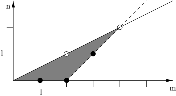
FIG. 1.: The $m$-$n$ plane. States to the right of the solid line are maximally chiral. The dashed line separates states with irrelevant tunneling (to the right) from states with relevant tunneling (to the left). The shaded region contains all maximally-chiral states with non-irrelevant tunneling: 010, 020, and 131 (dark circles). The states 121 and 242 which lie on the boundary of the maximally-chiral region are also shown (open circles).

The full Hamiltonian of the multilayer edge theory with tunneling can be written using Eqns. (32), (35), and (38):

$${\cal H}=\int_{-L/2}^{L/2}dx\,\left[{{1\over{4\pi}}v_{q}\,:\!\partial_{x}\phi_{q}\partial_{x}\phi_{-q}\!:+\sum_{j}{\lambda\over(2\pi a)^{\delta_{\lambda}}}\left({e^{i\alpha_{jq}\phi_{q}(x)}+\,\,{\rm h.c.}}\right)}\right],$$ (39)

where $a$ is a short distance cutoff. In the following sections we will be concerned with the $z$-axis conductivity of this theory, so we will need the form of the current operator along $z$. If $\rho^{(2D)}_{j}(x,t)$ is the two-dimensional charge density operator in layer $j$, the continuity equation can be written

$${\partial\over\partial t}\rho^{(2D)}_{j}(x,t)={1\over d}\left({{\cal J}^{z}_{j-1,j}(x,t)-{\cal J}^{z}_{j,j+1}(x,t)}\right)-\partial_{x}{\cal J}^{x}_{j}(x,t),$$ (40)

where ${\cal J}^{x}_{j}$ is the current density along the edge of layer $j$, ${\cal J}^{z}_{j,l}$ is the current density flowing from layer $j$ to layer $l$, and $d$ is the layer separation. Introducing the discrete Fourier transforms

$$\rho^{(2D)}(k,q,t)=d\sum_{j}\int dx\,e^{-iqj}e^{-ikx}\rho^{(2D)}_{j}(x,t),$$ (41)

with an analogous definition for ${\cal J}^{x}(k,q,t)$, and

$${\cal J}^{z}(k,q,t)=d\sum_{j}\int dx\,e^{-iq(j-1/2)}e^{-ikx}{\cal J}^{z}_{j-1,j}(x,t),$$ (42)

where the allowed values of the dimensionless $z$-momentum $q$ are given in Eq. (27), the continuity equation (40) becomes

$${\partial\over\partial t}\rho^{(2D)}(k,q,t)=-{2i\over d}\sin(q/2){\cal J}^{z}(k,q,t)-ik{\cal J}^{x}(k,q,t).$$ (43)

Note $\rho_{j}^{(2D)}(x,t)\equiv(1/d)\rho_{j}(x,t)$, where $\rho_{j}$ is given in Eq. (23). Therefore, at $k=0$ we can write Eq. (43) as

$${\cal J}^{z}(k=0,q,t)=-{d\over 2\sin(q/2)}\left[{H,\rho^{(2D)}(k=0,q,t)}\right].$$ (44)

Evaluating the commutator with the help of Eqns. (22), (23), and (35), we find

$$I^{z}(t)\equiv{\cal J}^{z}(k=0,q=0,t)=-{i\lambda d\over(2\pi a)^{\delta_{\lambda}}}\sum_{j}\int_{-L/2}^{L/2}dx\,\left[{e^{i\alpha_{jq^{\prime}}\phi_{q^{\prime}}(x,t)}-\,\,{\rm h.c.}}\right].$$ (45)

This expression will be used to calculate the $z$-axis conductivity of the multilayer system.

IV Marginal Tunneling Cases

We know there are only two maximally-chiral states with marginal tunneling: 131 and the bosonic state 020. In this section we begin by showing that in the absence of disorder these states exhibit insulating behavior in the vertical direction, i.e., $\sigma^{zz}(\omega)$ is identically zero for all frequencies at $T=0$. We will then find that adding disorder to the edge theory increases the vertical conductivity, and therefore the surface behaves like a “chiral semi-metal”. We conclude this section by considering how the transport is modified by nearest-neighbor density-density interactions.

A Clean Limit

Our discussion of the system in the absence of disorder will proceed in two steps. First, we derive a sum rule which relates the frequency integral of the conductivity to the expectation value of the tunneling term in the Hamiltonian. Next we prove that there exists a finite range of values for the tunneling amplitude $\lambda$, and the interaction strength $g$, for which the ground state in the presence of tunneling and interactions is identical to the ground state in the absence of tunneling and interactions. We then combine these two results to arrive at our conclusions about the zero temperature conductivity. We emphasize that this argument is non-perturbative in $\lambda$ and $g$. This is an important point since we do not have a quadratic form of the Hamiltonian for the multilayer state with marginal tunneling.

The conductivity sum rule is derived by considering the double commutator of the Hamiltonian with the charge density operator. Specifically, we calculate:

$$\left[{[{\cal H},\rho^{(2D)}(k=0,q,t)],\rho^{(2D)}(k=0,-q,t)}\right],$$ (46)

where the Hamiltonian is given in Eq. (39), and from Eqns. (23), (26), (30), (41), and $\rho_{j}^{(2D)}(x,t)=(1/d)\rho_{j}(x,t)$ we have

$$\rho^{(2D)}(k=0,q,t)={1\over 2\pi}\sqrt{N}\int_{-L/2}^{L/2}dx\,{1\over\sqrt{K_{q}}}\partial_{x}\phi_{q}(x,t).$$ (47)

Using the commutation relations for the fields $\phi_{q}(x)$ (31) it is a straightforward exercise to evaluate the commutator (46) with the help of Eqns. (39) and (47). One finds:

$$\left[{[{\cal H},\rho^{(2D)}(k=0,q,t)],\rho^{(2D)}(k=0,-q,t)}\right]=4\sin^{2}(q/2)\,{\cal H}_{\lambda},$$ (48)

where ${\cal H}_{\lambda}$ is the tunneling part of the Hamiltonian.

We next relate the expectation value of this double commutator to the integrated conductivity. The continuity equation (40) introduced in the previous section can be written

$$\rho^{(2D)}(k=0,q,t)={2\over d}\sin(q/2)\int{d\omega\over 2\pi}\int dt^{\prime}\,{e^{-i\omega(t-t^{\prime})}\over\omega}{\cal J}^{z}(k=0,q,t).$$ (49)

Suppressing the argument $k=0$, using $[{\cal H},\rho]=-i\partial\rho/\partial t$, and taking the expectation value of Eq. (49) we find

$$\left\langle{\left[{[{\cal H},\rho^{(2D)}_{j}(q,t)],\rho^{(2D)}_{j}(-q,t)}\right]}\right\rangle={4\over d^{2}}\sin^{2}(q/2)\int{d\omega\over 2\pi}\int dt\,e^{i\omega t}\langle[{\cal J}^{z}(q,0),{\cal J}^{z}(-q,t)]\rangle.$$ (50)

If we take the expectation value of Eq. (48), and use it to eliminate the l.h.s. of Eq. (50) we find in the limit $q\rightarrow 0$:

$$\langle{\cal H}_{\lambda}\rangle={4\over d^{2}}\int{d\omega\over 2\pi}\int dt\,e^{i\omega t}\langle[I^{z}(0),I^{z}(t)]\rangle,$$ (51)

where we have used $I^{z}(t)={\cal J}^{z}(q=0,t)$. The Kubo formula relates the commutator appearing in this expression to the $z$-axis conductivity:

$$\Re e\,\sigma^{zz}(\omega)={1\over 2\omega}{1\over NLd}\int dt\,e^{i\omega t}\langle[I^{z}(t),I^{z}(0)]\rangle.$$ (52)

Thus we arrive at the final form of the sum rule

$$\int d\omega\,\Re e\,\sigma^{zz}(\omega)=-{\pi d\over NL}\langle{\cal H}_{\lambda}\rangle.$$ (53)

This is an exact relation valid at any temperature. It applies to all multilayer states, even in the presence of disorder, regardless of the relevancy of the tunneling term.

Next we turn our attention to proving the stability of the ground state in the presence of interlayer tunneling and interactions. We will describe in detail the case of the bosonic 020 state. A proof along the same lines can be constructed for the 131 state. We begin by writing the Hamiltonian of the 020 edge theory in terms of the original radius $R=1$ Bose fields $u_{j}(x)$:

$${\cal H}_{020}=\int_{-L/2}^{L/2}dx\,\sum_{j}\left[{{v\over 16\pi}\,:\!(\partial_{x}u_{j})^{2}\!:\,+{g\over 8\pi}\partial_{x}u_{j}\partial_{x}u_{j+1}+{\lambda\over(2\pi a)^{2}}\left({e^{i(u_{j}-u_{j+1})}+\,\,{\rm h.c.}}\right)}\right].$$ (54)

Instead of performing the discrete Fourier transformation along $z$ (26) we simply rescale the fields, defining $u_{j}(x)=\sqrt{2}\varphi_{j}(x)$, where $\varphi_{j}(x)$ are radius $R=1/\sqrt{2}$ chiral bosons. We can then define a set of $N$ $\widehat{su}(2)_{1}$ Kac-Moody (KM) currents:

$$J^{z}_{j}(x)={1\over 2\pi\sqrt{2}}\partial_{x}\varphi_{j}(x),\qquad J^{\pm}_{j}(x)=J^{x}_{j}\pm iJ^{y}_{j}={1\over 2\pi a}e^{\mp i\sqrt{2}\varphi_{j}(x)},$$ (55)

in terms of which the Hamiltonian (54) can be written

$${\cal H}_{020}=\int_{-L/2}^{L/2}dx\,\left[{{\pi v\over 6}\,:\!\left[{{\bf J}_{j}(x)}\right]^{2}\!:\,+\pi gJ^{z}_{j}(x)J^{z}_{j+1}(x)}\right.$$ (56)

$$\left.{{}+\lambda(J^{-}_{j}(x)J^{+}_{j+1}(x)+J^{-}_{j+1}(x)J^{+}_{j}(x))}\right],$$ (57)

where we have employed the identity

$$\int_{-L/2}^{L/2}dx\,\,:\!\left[{J^{z}(x)}\right]^{2}\!:\,=\int_{-L/2}^{L/2}dx\,{1\over 3}\,:\!\left[{{\bf J}(x)}\right]^{2}\!:.$$ (58)

Consider the theory without interactions, $g=0$, and without tunneling $\lambda=0$. The zero-energy ground state of this Hamiltonian, $|0\rangle$, is formed by taking the tensor product of the highest-weight state of the spin-0 irreducible representation of each $\widehat{su}(2)_{1}$ algebra. Thus, the ground state satisfies

$$J_{j,n}^{a}|0\rangle=0,\,{\rm for}\quad\forall\,\,j;\quad a=x,y,z;\quad n\geq 0,$$ (59)

where the Fourier components of the currents are defined by

$$J^{a}_{j,n}\equiv\int_{-L/2}^{L/2}dx\,J^{a}_{j}(x)e^{-2\pi inx/L},\quad n\in{\mathchoice{{\sf Z\hskip-4.49997pt{}Z}}{{\sf Z\hskip-4.40002pt{}Z}}{{\sf Z\hskip-3.39996pt{}Z}}{{\sf Z\hskip-3.50006pt{}Z}}},$$ (60)

and obey the algebra

$$[J^{a}_{i,n},J^{b}_{j,m}]={n\over 2}\delta_{ij}\delta^{ab}\delta_{n+m,0}+i\delta_{ij}\epsilon^{abc}J^{c}_{j,n+m}.$$ (61)

Using Eqns. (57) and (60) we can write the Hamiltonian as

$${\cal H}_{020}=\left[{{\pi v\over 6L}\,:\!J^{a}_{j,n}J^{a}_{j,-n}\!:\,+{\pi g\over L}J^{z}_{j,n}J^{z}_{j+1,-n}+{\lambda\over L}(J^{-}_{j,n}J^{+}_{j+1,-n}+J^{-}_{j+1,n}J^{+}_{j,-n})}\right].$$ (62)

For later reference we also record the expression for the current operator in terms of the KM generators

$$I^{z}=-{i\lambda d\over L}\left[{J^{-}_{j,n}J^{+}_{j+1,-n}-J^{-}_{j+1,n}J^{+}_{j,-n}}\right].$$ (63)

From Eqns. (59) and (62) we see that not only is $|0\rangle$ the zero-energy ground state of the Hamiltonian with $g=\lambda=0$, it is a zero-energy eigenstate of the Hamiltonian for all $g$ and $\lambda$:

$${\cal H}_{020}|0\rangle=0.$$ (64)

Of course, this does not mean that $|0\rangle$ is the ground state of the Hamiltonian with non-zero $g$ and $\lambda$. To establish this we now demonstrate that for a range of $g$ and $\lambda$ the Hamiltonian is positive semi-definite. For $\lambda>0$, $g>0$, we rewrite Eq. (57) as

$${\cal H}_{020} = \int_{-L/2}^{L/2}dx\,\biggl{\{}{\pi g\over 2}:\!\left({J}^{z}_{j}+{J}^{z}_{j+1}\right)^{2}\!:\,+{\lambda\over 2}\left[:\!\left({J}^{-}_{j}+{J}^{-}_{j+1}\right)\left({J}^{+}_{j}+{J}^{+}_{j+1}\right)\!:+(J^{+}\leftrightarrow J^{-})\right]$$ (66)

$$+\left({\pi v\over 2}-\pi g\right)\,:\!\left[{J^{z}_{j}(x)}\right]^{2}\!:-\lambda\left[:\!{J}^{-}_{j}(x){J}^{+}_{j}(x)\!:+:\!{J}^{+}_{j}(x){J}^{-}_{j}(x)\!:\right]\biggr{\}}.$$

The two terms in the first line are clearly non-negatively defined, while the terms in the second line can be shown to be non-negatively defined for $v>2g+8\lambda/\pi$ using Eq. (58) and the basic identity

$$\left({{\bf J}_{j}}\right)^{2}=\left({J^{z}_{j}}\right)^{2}+{1\over 2}(J^{+}_{j}J^{-}_{j}+J^{-}_{j}J^{+}_{j}).$$ (67)

An analogous construction can be done for $\lambda<0$ or $g<0$, and we conclude that the Hamiltonian (57) is positive semi-definite provided

$$2|g|+{8}|\lambda|/\pi<{v}.$$ (68)

This is also the sufficient condition for the stability of the original ground state, as follows from our previous result that the Hamiltonian annihilates the original ground state $|0\rangle$.

Note that the normal ordering does not present a complication because it amounts to subtracting off the unit operator times the expectation value of the Hamiltonian in the state $|0\rangle$, which is zero. Therefore, since the Hamiltonian is positive semi-definite and we know the state $|0\rangle$ is a zero-energy eigenstate, it follows that $|0\rangle$ is the ground state of the Hamiltonian provided Eq. (68) is satisfied.

We can now combine the sum rule with our knowledge of the exact ground state to say something about the conductivity. At zero temperature the expectation value on the r.h.s. of the sum rule (53) is a ground state expectation value. Since we know the ground state $|0\rangle$ is unchanged by tunneling and interactions and $\langle 0|{\cal H}_{1}|0\rangle=0$ we can conclude

$$\int d\omega\,\Re e\,\sigma^{zz}(\omega)=0.$$ (69)

The real part of $\sigma^{zz}(\omega)$ is dissipative and hence it cannot be negative. Therefore, from Eq. (69) we have

$$\sigma^{zz}(\omega)=0.$$ (70)

We reiterate that this is an exact statement for the clean 020 multilayer at $T=0$ provided $g$ and $\lambda$ satisfy Eq. (68). As we mentioned above, a similar result can be shown to hold for the 131 state, the other maximally-chiral state with marginal tunneling. The condition for the stability of the ground state of the 131 edge theory is also given by Eq. (68). In the next section we will explore what happens when we add disorder to these systems.

B Disordered Case

In the previous section we found that the clean multilayer with marginal tunneling exhibits insulating behavior. In this section we study the marginal tunneling case in the presence of disorder. We perform a perturbative calculation of the vertical conductivity via the Kubo formula, finding that disorder increases the conductivity.

In Section III we discussed the general edge theory of clean multilayer systems. Our first task is to add disorder to this model. We will then use the Kubo formula to find the $z$-axis conductivity.

The disorder we consider is a random scalar potential $V_{j}(x)$ in each layer $j$, which couples to the Bose fields via the charge density

$${\cal H}_{V}=\int_{-L/2}^{L/2}dx\,V_{j}(x)\rho_{j}(x)=\int_{-L/2}^{L/2}dx\,{1\over 2\pi}V_{j}(x)K_{jk}\partial_{x}u_{k}(x).$$ (71)

We assume $V_{j}(x)$ is a Gaussian random variable, uncorrelated between different layers, but for now we will not specify how it is correlated within the same layer.

Using the Fourier transformation (26) and rescaling (30) of the Bose fields we can write Eq. (71) as

$${\cal H}_{V}=\int_{-L/2}^{L/2}dx\,{1\over 2\pi}{1\over\sqrt{K_{q}}}V_{q}\partial_{x}\phi_{-q}(x),$$ (72)

where

$$V_{q}(x)={1\over\sqrt{N}}\sum_{j}e^{-iqj}V_{j}(x).$$ (73)

Recalling the form of the clean multilayer edge theory from Section III, our full Hamiltonian is

$${\cal H} = \int_{-L/2}^{L/2}dx\,\left[{{1\over{4\pi}}v_{q}\,:\!\partial_{x}\phi_{q}\partial_{x}\phi_{-q}\!:\,+\sum_{j}{\lambda\over(2\pi a)^{2}}\left({e^{i\alpha_{jq}\phi_{q}(x)}+\,\,{\rm h.c.}}\right)}\right.$$ (75)

$$\left.{{}+{1\over 2\pi}{1\over\sqrt{K_{q}}}V_{q}\partial_{x}\phi_{-q}(x)}\right].$$

We move the disorder term into the phase of the tunneling amplitude by shifting the bosons:

$$\phi_{q}\mapsto\phi_{q}+{1\over v_{q}\sqrt{K_{q}}}\int^{x}dy\,V_{q}(y).$$ (76)

If we define the phases

$$\gamma_{j}(x)\equiv-{1\over\sqrt{N}}\sum_{q}e^{iqj}(1-e^{iq}){1\over v_{q}}\int^{x}dy\,V_{q}(y),$$ (77)

then with Eq. (76) the Hamiltonian (75) is

$${\cal H}=\int_{-L/2}^{L/2}dx\,\left[{{1\over 4\pi}v_{q}\,:\!\partial_{x}\phi_{q}\partial_{x}\phi_{-q}\!:\,+{\lambda\over(2\pi a)^{2}}\sum_{j}\left({e^{i\gamma_{j}(x)}e^{i\alpha_{jq}\phi_{q}(x)}+\,\,{\rm h.c.}}\right)}\right],$$ (78)

and the current operator (45) becomes

$$I^{z}=-{i\lambda d\over(2\pi a)^{2}}\sum_{j}\int_{-L/2}^{L/2}dx\,\left[{e^{i\gamma_{j}(x)}e^{i\alpha_{jq}\phi_{q}(x)}-\,\,{\rm h.c.}}\right].$$ (79)

We are now in a position to calculate the $z$-axis conductivity. We will first evaluate the Matsubara two-point function of the current operator (79). Since Eq. (78) is a theory of $N$ interacting chiral bosons, the best we can do is a perturbative calculation in the tunneling amplitude $\lambda$. Although we will work perturbatively in $\lambda$, we will be treating the disorder exactly. We thus expect the ${\cal O}(\lambda^{2})$ result to be reliable, since the disorder essentially randomizes the phase of the electrons between tunneling events. More formally, if the tunneling amplitude is a coordinate-dependent, delta-correlated random variable, then the RG flow (37) is modified to

$${d\Delta\over d\ell}=(3-2\delta_{\lambda})\Delta,$$ (80)

where $\Delta$ is the variance of the tunneling. Thus for $\delta_{\lambda}=2$ we would conclude that the tunneling is irrelevant. The combination $\lambda e^{i\gamma_{j}(x)}$ that appears in the Hamiltonian (78) is in general not delta-correlated, as we will discuss below, but since the case of $x$-independent tunneling is marginal we expect any departure from uniformity makes the tunneling irrelevant and therefore justifies a perturbative expansion in $\lambda$.

Using the expression for the current operator (79) we evaluate the Matsubara two-point function

$${\sf C}(\tau) = -\langle T_{\tau}I^{z}(\tau)I^{z}(0)\rangle$$ (81)

$$= {d^{2}\lambda^{2}\over L^{4}}\int dx\,dx^{\prime}\,\sum_{j,k}\left\langle{T_{\tau}\left({e^{i\gamma_{j}(x)}\,:\!e^{i\alpha_{jq}\phi_{q}(\tau,x)}\!:\,-\,e^{-i\gamma_{j}(x)}\,:\!e^{-i\alpha_{jq}\phi_{q}(\tau,x)}\!:}\right)}\right.$$ (83)

$$\left.{{}\times\left({e^{i\gamma_{k}(x^{\prime})}\,:\!e^{i\alpha_{kq}\phi_{q}(0,x^{\prime})}\!:\,-\,e^{-i\gamma_{k}(x^{\prime})}\,:\!e^{-i\alpha_{kq}\phi_{q}(0,x^{\prime})}\!:}\right)}\right\rangle,$$

where we have normal-ordered the vertex operators. Note that because the current operator (79) has a factor of $\lambda$ out front, there is an explicit factor of $\lambda^{2}$ in Eq. (83), and therefore to find this function to order $\lambda^{2}$ we can evaluate the expectation value using the $\lambda=0$ Hamiltonian. One finds that only the cross terms in the product of the current operators give non-vanishing contributions, and only when $j=k$. The terms have the form

$$-\left\langle{T_{\tau}\,:\!e^{i\alpha_{jq}\phi_{q}(\tau,x)}\!:\,:\!e^{-i\alpha_{jq}\phi_{q}(0,x^{\prime})}\!:}\right\rangle$$ (85)

$$=\prod_{q}{L^{\alpha^{2}_{q}}\over\left[{(2\beta iv_{q})\sinh\left({{\pi\over\beta v_{q}}(x-x^{\prime}+iv_{q}\tau+ia\,{\rm sgn}\,\tau)}\right)}\right]^{\alpha_{q}^{2}}},$$

where $\alpha_{q}^{2}\equiv\alpha_{jq}\alpha_{j-q}$, with no sum on $j$. This is a very complicated function; a great simplification occurs if the eigenmode velocities, $v_{q}$, are identical for all $q$. From the expression for $v_{q}$ (34) we see that this occurs when $g=nv/m$. For the two multilayer states with marginal tunneling, 020 and 131, this condition gives $g=0$ and $g=v/3$, respectively. We will refer to the case where $v_{q}$ is independent of $q$ as the “solvable point.” For 020 it corresponds to no density-density couplings between neighboring layers while for 131 it occurs at a non-zero value of the density-density interaction strength. Note that for more general forms of the matrices $K$ and $U$, i.e., not tridiagonal, the solvable point corresponds to $U\propto K$.

Working at the solvable point, writing $v_{q}\equiv v_{0}$, and using our knowledge of the scaling dimension of the tunneling operator (38),

$$\sum_{q}\alpha_{q}^{2}=\sum_{q}\alpha_{jq}\alpha_{j-q}=2\delta_{\lambda}=4,$$ (86)

we find upon disorder averaging Eq. (83)

$$\overline{\sf C}(\tau)=-{2d^{2}\lambda^{2}\over(2\beta v_{0})^{4}}\sum_{j}\int dx\,dx^{\prime}\,{W_{j}(x,x^{\prime})\over\left[{\sinh\left({{\pi\over\beta v_{0}}(x-x^{\prime}+iv_{0}\tau+ia\,{\rm sgn}\,\tau)}\right)}\right]^{4}},$$ (87)

where we have defined the function

$$W_{j}(x,x^{\prime})\equiv\overline{e^{i[\gamma_{j}(x)-\gamma_{j}(x^{\prime})]}}.$$ (88)

If we take the correlation function of the scalar potential to be

$$\overline{V_{j}(x)V_{k}(x^{\prime})}=\delta_{jk}Z(x-x^{\prime}),$$ (89)

then using the definition of the phase $\gamma_{j}(x)$ (77) we find that the function $W_{j}(x,x^{\prime})$ can be written

$$W_{j}(x,x^{\prime})=\exp\left[{-{1\over v_{0}^{2}}\int_{x}^{x^{\prime}}dy_{1}\,\int_{x}^{x^{\prime}}dy_{2}\,Z(y_{1}-y_{2})}\right],$$ (90)

Note that $W_{j}(x,x^{\prime})\equiv W(x-x^{\prime})$ is independent of $j$ and depends only on the magnitude of the relative coordinate $|x-x^{\prime}|$. Therefore the sum over $j$ in Eq. (87) just gives a factor of the number of layers, $N$, and we can replace the integration over $x$ and $x^{\prime}$ by an integration over the average coordinate, which gives a factor of $L$, and an integration over the relative coordinate $y=x-x^{\prime}$. If we define the Fourier transform of the function $W(x)$:

$${\widetilde{W}}(k)\equiv\int dx\,e^{-ikx}W(x),$$ (91)

then we can write Eq. (87) as

$$\overline{\sf C}(\tau)=-{2d^{2}NL\lambda^{2}\over(2\beta v_{0})^{4}}\int{dk\over 2\pi}{\widetilde{W}}(k)\int dy\,{e^{iky}\over\left[{\sinh\left({{\pi\over\beta v_{0}}(y+iv_{0}\tau+ia\,{\rm sgn}\,\tau)}\right)}\right]^{4}}$$ (92)

The factor of $L$ in this expression will cancel against the factor of $1/L$ in the Kubo formula (52), and in anticipation of this we have extended the range of the $y$ integral to include the entire real axis since we are interested in the result in the limit where the system size $L\rightarrow\infty$. The integration over $y$ can now be performed by the method of residues. The integrand has fourth-order poles on the imaginary $y$-axis at the points $y_{n}=i[v_{0}(\beta n-\tau)-a\,{\rm sgn}\,\tau]$ for integer $n$, and is exponentially small in the upper (lower) half plane for $k>0$ ($k<0$). One finds

$$\int dy\,{e^{iky}\over\left[{\sinh\left({{\pi\over\beta v_{0}}(y+iv_{0}\tau+ia\,{\rm sgn}\,\tau)}\right)}\right]^{4}}={\pi\over 3}\left[{4\left({\beta v_{0}k\over\pi}\right)+\left({\beta v_{0}k\over\pi}\right)^{3}}\right]{e^{v_{0}k\tau}\over e^{\beta v_{0}k}-1}.$$ (93)

We now Fourier transform Eq. (92) with respect to the imaginary time $\tau$,

$$\overline{\sf C}(\omega_{n}) = \int_{0}^{\beta}d\tau\,e^{i\omega_{n}\tau}\overline{\sf C}(\tau)$$ (94)

$$= -{d^{2}\lambda^{2}NL\over 48\pi^{4}v_{0}^{4}}\int dp\,{\widetilde{W}}(p/v_{0}){p^{3}+4\pi^{2}p/\beta^{2}\over i\omega_{n}+p},$$ (95)

where we have changed the integration variable to $p\equiv v_{0}k$. Analytically continuing ($i\omega_{n}\mapsto\omega+i0^{+}$) we find

$$\overline{\cal C}(\omega) = -i\int_{0}^{\infty}dt\,e^{i\omega t}\overline{\langle[I^{z}(t),I^{z}(0)]\rangle}$$ (96)

$$= -{d^{2}\lambda^{2}NL\over 48\pi^{4}v_{0}^{4}}\int dp\,{\widetilde{W}}(p/v_{0}){p^{3}+4\pi^{2}p/\beta^{2}\over\omega+p+i0^{+}}.$$ (97)

Using this result in the Kubo formula (52) with the help of the identity

$${1\over x\pm i0^{+}}={\cal P}{1\over x}\mp i\pi\delta(x),$$ (98)

and the observation that ${\widetilde{W}}(k)$ is real since $W(x)$ is an even function of $x$, we arrive finally at

$$\Re e\,\overline{\sigma^{zz}}(\omega)={\lambda^{2}d\over 48\pi^{3}v_{0}^{4}}(\omega^{2}+4\pi^{2}T^{2}){\widetilde{W}}(\omega/v_{0}).$$ (99)

This is our central result. It is the ${\cal O}(\lambda^{2})$ term in the vertical conductivity at the solvable point for both the 020 and 131 states at a finite temperature $T$, including potential disorder which enters through the function ${\widetilde{W}}(k)$. The imaginary part of the conductivity can of course be found from Eq. (99) by the usual dispersion relations[19].

Let us first consider the limit of a clean system, $V_{j}(x)\equiv 0$. From Eqns. (89) and (90), we see that in this case $W(x)=1$ and therefore ${\widetilde{W}}(k)=2\pi\delta(k)$. Hence from Eq. (99) we find

$$\Re e\,\sigma^{zz}(\omega)={\lambda^{2}d\over 6v_{0}^{3}}T^{2}\delta(\omega).$$ (100)

This is consistent with our result in Section IV A that the $z$-axis conductivity in the clean system vanishes at $T=0$. An interesting aspect of this result is that it is proportional to $\delta(\omega)$, i.e., the conductivity vanishes at all $\omega\neq 0$, and the DC conductivity is infinite. One question to ask is whether these features are a consequence of the fact that Eq. (100) is only the first non-vanishing term in a perturbative expansion in $\lambda$.

Although we cannot definitively answer the question about the finiteness of the DC conductivity beyond ${\cal O}(\lambda^{2})$, we can prove that at higher orders in $\lambda$ the conductivity cannot vanish at all $\omega\neq 0$. First we note that in the clean system the current operator commutes with the Hamiltonian in the absence of tunneling: $[I^{z},{\cal H}_{0}]=0$. For example, for the 020 state this can be seen from Eqns. (62) and (63), using the commutation relations for the Kac-Moody currents given in Eq. (61). Since the current operator commutes with ${\cal H}_{0}$, the expectation value of the current-current commutator evaluated using the $\lambda=0$ Hamiltonian vanishes, and therefore by the Kubo formula (52) the vertical conductivity must vanish for all non-zero frequencies. This explains why the conductivity is zero except at $\omega=0$ in Eq. (100). By the same reasoning we see that if the current operator commutes with the full Hamiltonian, $[I^{z},{\cal H}]=0$, then $\sigma^{zz}(\omega)$ would be zero for all $\omega\neq 0$ to all orders in $\lambda$. The converse of this is also true, i.e., if $\sigma^{zz}(\omega)$ is zero for all $\omega\neq 0$ then $[I^{z},{\cal H}]=0$. This is proven in Appendix D. For the multilayer edge theory with marginal tunneling: $[I^{z},{\cal H}]\neq 0$. For the 020 case this can be established using Eqns. (62) and (63). Therefore, since the current operator does not commute with the full Hamiltonian, we can conclude that $\sigma^{zz}(\omega)$ cannot be zero for all $\omega\neq 0$ for the clean 020 or 131 multilayers. Hence, we would expect that the $\delta(\omega)$ factor in Eq. (100) would be broadened by the higher-order corrections in $\lambda$. Recalling that $\lambda$ is dimensionless and the conductivity should not depend on the sign of $\lambda$, one plausible scenario is:

$$\Re e\,\sigma^{zz}(\omega)={\lambda^{2}d\over 6v_{0}^{3}}T\delta(\omega/T)\mapsto\,\,\,\,\sim{\lambda^{2}d\over 6v_{0}^{3}}T{\lambda^{2}\over(\omega/T)^{2}+{\cal O}(\lambda^{4})}.$$ (101)

This conjectured form has several interesting features. First, we find that the DC conductivity goes to zero with temperature as $T$. We expect this to be a generic feature of the exact result in $\lambda$ for the clean system, provided the DC conductivity is finite. This differs from the disordered system (99) where we find the DC conductivity vanishes as $T^{2}$. In addition, note that the $\omega\rightarrow 0$ limit of Eq. (101) is independent of the tunneling amplitude $\lambda$.

We now return to the result for $\overline{\sigma^{zz}}(\omega)$ in the presence of disorder (99). If the disorder is delta-correlated, the function $Z(x)$ defined in Eq. (89) is

$$Z(x)=\Delta\delta(x),$$ (102)

where $\Delta$ is the variance of the disorder. For this case $W(x)=\exp(-\Delta|x|/v_{0}^{2})$, which has a Fourier transform ${\widetilde{W}}(k)=(2\Delta/v_{0}^{2})/(k^{2}+(\Delta/v_{0}^{2})^{2})$, and hence (99) yields

$$\Re e\,\overline{\sigma^{zz}}(\omega)={\lambda^{2}d\Delta\over 24\pi^{3}v_{0}^{4}}{\omega^{2}+4\pi^{2}T^{2}\over\omega^{2}+(\Delta/v_{0})^{2}}.$$ (103)

Note that at zero temperature the conductivity vanishes in the DC limit. This conclusion is independent of the details of the disorder and holds as long as ${\widetilde{W}}(0)$ is finite. We also see that the conductivity approaches a constant as $\omega\rightarrow\infty$. This second feature is a consequence of taking the disorder to be delta-correlated. We see that $\overline{\sigma^{zz}}(\omega)$ goes to a constant at large $\omega$ because of the slow fall off of ${\widetilde{W}}(k)$, which is in turn caused by the non-analyticity of $W(x)$ at $x=0$. We shall now investigate how Eq. (103) is modified if the disorder has a finite correlation length.

As a first step, we determine the asymptotic form of the disorder-averaged phase, $W(x)$, at small and large $x$ when the scalar potential disorder has a finite correlation length. We return to the expression for the correlation function of the random potential (89) and write

$$Z(x)\equiv\Delta^{2}A(x/\ell_{0}),$$ (104)

where $\Delta$ is a parameter with the dimensions of energy that sets the strength of the disorder, $\ell_{0}$ is the correlation length of the disorder, and $A(z)$ is a dimensionless function which we take to have the properties: $A(0)=1$, $A(-z)=A(z)$, and

$$\int_{0}^{\infty}dz\,A(z)=1.$$ (105)

Now consider the disorder-averaged phase, $W(x)$, given in Eq. (90). For $|x|\ll\ell_{0}$, i.e., for distances small compared with the correlation length of the random potential, we can replace $Z(y_{1}-y_{2})$ by its value at $y_{1}-y_{2}=0$ and obtain:

$$W(\ell_{0}z)\approx e^{-(\Delta\ell_{0}z/v_{0})^{2}}\approx 1-\left({\Delta\ell_{0}z\over v_{0}}\right)^{2},\quad{\rm for}\quad|z|\ll 1.$$ (106)

In the opposite limit $|x|\gg\ell_{0}$ we change integration variables in Eq. (90) to $y_{c}=(y_{1}+y_{2})/2$ and $y_{r}=y_{1}-y_{2}$:

$$W(x)=\exp\left[{-{1\over v_{0}^{2}}\left({\int_{-|x|}^{0}dy_{r}\,(|x|+y_{r})Z(y_{r})+\int_{0}^{|x|}dy_{r}\,(|x|-y_{r})Z(y_{r})}\right)}\right].$$ (107)

Since $|x|/\ell_{0}\gg 1$ we can extend the integration over $y_{r}$ to infinity with small error. Using the symmetry of $A$ and defining

$$\zeta=\int_{0}^{\infty}dz\,zA(z),$$ (108)

we then find

$$W(\ell_{0}z)\approx\exp\left[{-2\left({\Delta\ell_{0}\over v_{0}}\right)^{2}(|z|-\zeta)}\right],\quad{\rm for}\quad|z|\gg 1.$$ (109)

We see that at short distances $W(x)$ is parabolic (106) while at long distances it decays exponentially (109). The presence of a finite correlation length for the random potential does not change the long distance behavior of $W(x)$, but it does “round out” the non-analyticity at $x=0$ present in the case of delta-correlated disorder. Generally, this is sufficient to make the function rapidly decaying as $\omega\rightarrow\infty$.

Having found the generic behavior of the function $W(x)$, we now choose a specific form:

$$W(x)={1\over\cosh(\xi x)},$$ (110)

characterized by the parameter $\xi$ which has the dimensions of an energy. This choice of $W(x)$ has several appealing features. First, it has the correct asymptotic forms at large and small values of $x$. Indeed, if we match the asymptotics of Eq. (110) to Eqns. (106) and (109) we find

$${\Delta\over v_{0}}=\xi,\quad\ell_{0}={1\over 2\xi}.$$ (111)

We see that for the choice of $W(x)$ in Eq. (110), the parameter $\xi$ is proportional to the strength of the disorder and inversely proportional to the correlation length. Hence this form allows us to explore the effect of a finite correlation length in the region $\Delta\ell_{0}\sim 1$.

A second advantage of Eq. (110) is that its Fourier transform can be evaluated in closed form. A straightforward computation gives

$${\widetilde{W}}(k)=\int dx\,{e^{-ikx}\over\cosh(\xi x)}={\pi/\xi\over\cosh\left({\pi k/2\xi}\right)}.$$ (112)

Using this result in the general form above for the conductivity (99) we find

$$\Re e\,\overline{\sigma^{zz}}(\omega)={\lambda^{2}d\over 48\pi^{2}v_{0}^{4}}{\omega^{2}+4\pi^{2}T^{2}\over\xi\cosh\left({\pi\omega/2\xi v_{0}}\right)}.$$ (113)

Comparing Eq. (113) with the expression for the conductivity in the case of delta-correlated disorder (103) we see that the finite correlation length gives a conductivity which exponentially decays to zero as $\omega\rightarrow\infty$ rather than approaching a nonzero value. This result for $\overline{\sigma^{zz}}$ (113) is shown in Fig. 2 at various temperatures. For large temperatures the conductivity is peaked around $\omega=0$, while at smaller temperatures the maximum occurs at a finite frequency.

FIG. 2.: The real part of the vertical conductivity for the 020 or 131 multilayer with disorder (113). The horizontal axis is frequency measured in units of the parameter $v_{0}\xi$. The temperatures of the curves, starting with the uppermost, are: $T/v_{0}\xi=0.25,0.2,0.15,0.1,0.01$.

C Effect of Interactions

In the preceding section we calculated the order $\lambda^{2}$ term in the $z$-axis conductivity of the multilayer states with marginal tunneling, 020 and 131, at the solvable point where the eigenmode velocities $v_{q}$ are independent of $q$. In this section we discuss how the zero-temperature result is modified away from the solvable point.

Since we will only consider $T=0$ in this section we shall work directly in real time $t$. The real-time zero-temperature analog of the expression for the Matsubara two-point function of the current operator (87) is

$$\overline{\cal C}(t)=-{2id^{2}\lambda^{2}NL\over(2\pi)^{4}}\int dy\,W(y)\prod_{q}{1\over(y-v_{q}t+ia\,{\rm sgn}\,t)^{\alpha_{q}^{2}}},$$ (114)

where from the definitions (77) and (88) we see that the expression for $W(x)$ in Eq. (90) is changed to

$$W(x)=\exp\left[{-\left({{2\over N}\sum_{q}{\sin^{2}(q/2)\over v_{q}^{2}}}\right)\int^{x}_{0}dy_{1}\,\int^{x}_{0}dy_{2}\,Z(y_{1}-y_{2})}\right].$$ (115)

The corresponding retarded correlation function is

$$\overline{{\cal C}^{R}}(t)=-{2id^{2}\lambda^{2}NL\over(2\pi)^{4}}\theta(t)\int dy\,W(y)\left[{\prod_{q}{1\over(y-v_{q}t+ia)^{\alpha_{q}^{2}}}-\prod_{q}{1\over(y-v_{q}t-ia)^{\alpha_{q}^{2}}}}\right].$$ (116)

We would now like to perform the $y$-integration. From Eq. (36) we see that the exponents appearing in Eq. (116) are

$$\alpha_{q}^{2}={2\over N}(3-\cos q-2\cos^{2}q),$$ (117)

and therefore, as a function of complex $y$, the first integrand in Eq. (116) has $N$ branch point singularities at the points $v_{q}t-ia$ and similarly for the second integrand at $v_{q}t+ia$. This is a complicated singularity structure, but observe that in the first term these branch points are all below the real axis, while in the second term they are all above the real axis. Hence, since $\sum_{q}\alpha_{q}^{2}$ is an integer, we can certainly choose branch cuts that lie entirely on one side of the real axis for each term. When we considered the solvable point in the previous section we were able to evaluate the conductivity for any disorder $W(y)$. We shall not attempt the same feat away from the solvable point. The evaluation of the $y$-integral in Eq. (116) is greatly simplified if $W(y)$ is a meromorphic function of $y$. One such function was discussed in the previous section (110), and for the remainder of this section we specialize to this form.

Using $W(y)=1/\cosh(\xi y)$ in Eq. (116), we can close the first term in the upper-half plane and the second term in the lower-half plane, avoiding all the complicated branch point singularities, and picking up the residues of the poles of $W(y)$. We find

$$\overline{{\cal C}^{R}}(t) = -i\theta(t)\langle\overline{[I^{z}(t),I^{z}(0)]}\rangle$$ (118)

$$= -{2id^{2}\lambda^{2}NL\over(2\pi)^{3}}\theta(t)\xi^{3}\sum_{r=-\infty}^{\infty}(-1)^{r}\prod_{q}{1\over[v_{q}\xi t-i\pi(r+1/2)]^{\alpha_{q}^{2}}}.$$ (119)

Therefore, from the Kubo formula (52) we arrive at

$$\Re e\,\overline{\sigma^{zz}}(\omega)={\lambda^{2}d\over(2\pi)^{3}}{\xi^{3}\over\omega}\sum_{r=-\infty}^{\infty}(-1)^{r}\int dt\,e^{i\omega t}\prod_{q}{1\over[v_{q}\xi t-i\pi(r+1/2)]^{\alpha_{q}^{2}}}.$$ (120)

This is certainly far from a closed form result, but it is a convenient form for extracting the high and low frequency asymptotics of the conductivity. At large (positive) $\omega$ the asymptotic form is determined by the closest singularity to the real axis in the upper half of the complex $t$ plane. From Eq. (120) this clearly occurs a finite distance away from the real-$t$ axis and we find

$$\Re e\,\overline{\sigma^{zz}}(\omega)\stackrel{{\scriptstyle\omega\rightarrow\infty}}{{\longrightarrow}}\exp\left[{-{\pi\omega\over 2\xi v_{\rm max}}}\right],$$ (121)

where $v_{\rm max}$ is the maximum of $v_{q}$ over $q$. For the 020 state we see from the expression for $v_{q}$ (34) that at the solvable point ($g=0$) $v_{0}=v/2$ while away from the solvable point ($g>0$) $v_{\rm max}=v/2+g$. Comparing Eq. (121) with the asymptotic form of Eq. (113):

$$\Re e\,\overline{\sigma^{zz}}(\omega)\stackrel{{\scriptstyle\omega\rightarrow\infty}}{{\longrightarrow}}\exp\left[{-{\pi\omega\over 2\xi v_{0}}}\right],$$ (122)

we find that one effect of interactions at $T=0$ is to soften the exponential decay of the conductivity at large frequencies.

Returning to Eq. (120), we now consider the behavior at small frequencies. If we assume $\omega>0$ we can close the $t$ integral in the upper-half plane because the integrand is exponentially small there. Hence all the terms with $r<0$ give no contribution. For each $r\geq 0$ there remains $N$ branch point singularities in the upper-half plane enclosed by the contour. Since we are interested in small $\omega$ we stretch the integration contour into a large circle so that everywhere along the contour $|t|$ is very large. We can then expand the integrand in powers of $1/t$ and integrate term-by-term:

$$\int dt\,e^{i\omega t}\prod_{q}{1\over[v_{q}\xi t-i\pi(r+1/2)]^{\alpha_{q}^{2}}}$$ (125)

$$=\oint dt\,e^{i\omega t}\left({\prod_{q}{1\over v_{q}^{\alpha_{q}^{2}}}}\right){1\over(\xi t)^{4}}\left[{1+{i\pi(r+1/2)\over\xi t}\sum_{q}{\alpha_{q}^{2}\over v_{q}}+{\cal O}\left({1\over t^{2}}\right)}\right]$$

$$={\pi\over 3}\left({\prod_{q}{1\over v_{q}^{\alpha_{q}^{2}}}}\right){\omega^{3}\over\xi^{4}}\left[{1-{\pi\over 4}{\omega\over\xi}(r+1/2)\sum_{q}{\alpha_{q}^{2}\over v_{q}}+{\cal O}(\omega^{2})}\right].$$

If we retain only the lowest term in $\omega$ in this expansion, we note that upon substituting this into Eq. (120) we would encounter the divergent sum

$$\sum_{r=0}^{\infty}(-1)^{r}.$$ (126)

By considering the solvable point, where $v_{q}=v_{0}$ independent of $q$, it is clear that the proper regularization of this sum is

$$\sum_{r=0}^{\infty}(-1)^{r}=\lim_{\delta\rightarrow 0}\sum_{r=0}^{\infty}(-e^{-\delta})^{r}=\lim_{\delta\rightarrow 0}{1\over 1+e^{-\delta}}={1\over 2},$$ (127)

and thus from Eqns. (120), (125), and (127) we have

$$\Re e\,\overline{\sigma^{zz}}(\omega)\stackrel{{\scriptstyle\omega\rightarrow 0}}{{\longrightarrow}}{\lambda^{2}d\over 48\pi^{2}}\left({\prod_{q}{1\over v_{q}^{\alpha_{q}^{2}}}}\right){\omega^{2}\over\xi}.$$ (128)

Comparing this with the small frequency asymptotics of Eq. (113) at $T=0$:

$$\Re e\,\overline{\sigma^{zz}}(\omega)\stackrel{{\scriptstyle\omega\rightarrow 0}}{{\longrightarrow}}{\lambda^{2}d\over 48\pi^{2}}{1\over v_{0}^{4}}{\omega^{2}\over\xi},$$ (129)

we see that the interactions do not modify the result that the conductivity goes to zero in the DC limit at zero temperature. While the power of $\omega$ is the same in Eqns. (128) and (129), the interactions do modify the prefactor.

To summarize, we have considered how interactions away from the solvable point modify the vertical conductivity at $T=0$. It should be noted that in arriving at Eq. (120) the interactions were treated exactly. We find that at large frequencies the interactions soften the decay of the conductivity, but it remains exponential, while at small frequencies the interactions do not change the frequency exponent of the conductivity. We remark that the difficulty encountered when attempting to apply the method presented in this section to investigate the effect of interactions at a finite temperature is that in the finite-$T$ version of Eq. (116) there are complicated branch point singularities on both sides of the real-$y$ axis, see Eq. (85). Nevertheless, we believe that even at a finite temperature the asymptotics of $\sigma^{zz}(\omega)$ are not modified by interactions.

V Irrelevant Tunneling

In the previous section we have been concerned exclusively with the case of marginal tunneling, namely the 020 and 131 multilayer states. The calculation presented in Section IV B can readily be extended to the more general case of the $nmn$ state. Essentially the only change in the computation is that the scaling dimension of the tunneling operator, $\delta_{\lambda}=m-n$, differs from its marginal value of 2. Therefore, the poles in the complex $y$-plane for the integrand in Eq. (93) are now of order $2(m-n)$. One finds that for the solvable point $g=nv/m$:

$$\Re e\,\overline{\sigma^{zz}_{nmn}}(\omega)={\lambda^{2}d\over(2\pi)^{2\delta_{\lambda}-1}v_{0}^{2\delta_{\lambda}}}{{\widetilde{W}}(\omega/v_{0})\over(2\delta_{\lambda}-1)!}\prod_{k=1}^{\delta_{\lambda}-1}[\omega^{2}+(2\pi kT)^{2}].$$ (130)

For the case of relevant tunneling, $\delta_{\lambda}=m-n=1$, the product over $k$ is absent in Eq. (130), and if we use ${\widetilde{W}}(\omega/v_{0})=(2\Delta)/(\omega^{2}+(\Delta/v_{0})^{2})$ appropriate for delta-correlated disorder we reproduce the behavior of the chiral metal.

In the remaining cases, $\delta_{\lambda}\geq 2$, we see at $T=0$ the conductivity vanishes as $\omega\rightarrow 0$ as $\omega^{2(\delta_{\lambda}-1)}$, and at $\omega=0$ it vanishes with temperature as $T^{2(\delta_{\lambda}-1)}$. In the absence of interlayer correlations, i.e., for the $0m0$ state, this means the DC conductivity obeys $\sigma^{zz}\sim T^{2m-2}$. This disagrees with the result of Balents and Fisher, who find by a scaling argument that $\sigma^{zz}\sim T^{2m-3}$[4]. While it is unclear whether Balents and Fisher have in mind the clean system or the disordered system, we believe the reconciliation of this discrepancy is that, as we found for the marginal case, the temperature scaling of the DC conductivity is different in the clean and disordered systems. If we consider the clean limit of Eq. (130) by writing ${\widetilde{W}}(\omega/v_{0})=(v_{0}/T)\delta(\omega/T)$, and then conjecture that the interactions broaden the delta function, we find:

$$\Re e\,\overline{\sigma^{zz}_{nmn}}(\omega)\propto{\lambda^{2}d\over T}{g\over(\omega/T)^{2}+{\cal O}(g^{2})}\prod_{k=1}^{\delta_{\lambda}-1}[\omega^{2}+(2\pi kT)^{2}],$$ (131)

where $g$ is the dimensionless interaction strength. The broadening of the delta function by interactions is suggested by the fact that the nearest-neighbor density-density interaction Hamiltonian does not commute with the current operator $I^{z}$. For the case of the $0m0$ state the DC conductivity of Eq. (131) goes to zero as $T^{2m-3}$, in agreement with Balents and Fisher.

Finally, returning to the disordered case (130), we see that for the 050 state the DC conductivity scales as $T^{8}$, while for 131 it scales as $T^{2}$ (99). Recall from Eq. (5) that both of these states occur at the same electron density, $\nu=1/5$ per layer. In their numerical work, QJM found a phase transition between these states as the layer separation $d$ was varied. The significant difference in the temperature scaling of the DC vertical conductivity in these states suggests a way to experimentally detect this phase transition.

VI Fermionization

In certain special cases the multilayer edge theory can be solved exactly. The case of $N=2$ layers is discussed extensively elsewhere[11, 12], and examples of exact solutions for $N=4$ layers are given in Appendix B. A potentially useful first step to solving the edge theory for arbitrary $N$ is to find a fermionic representation. In this section we discuss the fermionization of the edge theory for an arbitrary number of layers $N$. In some cases the procedure involves the introduction of auxiliary degrees of freedom as discussed in Ref. [11].

We begin with the observation that the scaling dimension (38) of the tunneling operator is always an integer. This underlies the fact that the chiral Hamiltonian (39) can be fermionized exactly, with the tunneling term expressed as a product of Fermi operators whose number equals twice the scaling dimension.

The usual mapping between chiral radius-one bosons and fermions requires independent bosonic fields. Even though we are interested in correlated states with non-trivial commutators (22), these can be readily diagonalized by a linear transformation. For example, for the 131 state we can write

$$u_{j}=\varphi_{j-1/2}+\varphi_{j}+\varphi_{j+1/2},\quad j=1,2,\ldots,N$$ (132)

where the $2N$ bosons $\varphi_{j}$ with integer and half-integer indices have the usual commutation relations $[\varphi_{i}(x),\,\varphi_{j}(x^{\prime})]=i\pi\,\delta_{ij}\,{\rm sgn}(x-x^{\prime})$. Clearly, Eq. (132) is not a canonical transformation because the number of degrees of freedom has been doubled. This formal difficulty can be circumvented if we introduce an independent set of auxiliary bosons with half-integer indices $\tilde{u}_{i+1/2}$, $i=1,2,\ldots,N$ with identical commutation relations,

$$[\tilde{u}_{i+1/2}(x),\,\tilde{u}_{j+1/2}(x^{\prime})]=i\pi\,K_{ij}\,{\rm sgn}(x-x^{\prime}),\quad[u_{i}(x),\,\tilde{u}_{j+1/2}(x^{\prime})]=0.$$ (133)

Then, we can further write for the 131 state

$$\tilde{u}_{j+1/2}=-\varphi_{j}+\varphi_{j+1/2}-\varphi_{j+1},$$ (134)

and the transformation $u_{i},{\tilde{u}}_{i+1/2}\mapsto\varphi_{j}$ becomes canonical.

At the end of a calculation the auxiliary degrees of freedom need to be projected out. Such a projection has been explicitly carried out by us in Ref. [11] for the simpler case of correlated quantum Hall bilayers. However, since the auxiliary degrees of freedom are independent of the physical ones, all quantum-mechanical averages involving physical quantities will automatically be correct, independent of the Hamiltonian chosen for the additional bosons $\tilde{u}_{i+1/2}$. In the following we select this Hamiltonian in the form (21), i.e., identical to that for the physical bosonic fields sans the tunneling term. In this case, the transformations (132) and (134) give

$${\cal H}_{131} = \int_{-L/2}^{L/2}dx\,\Biggl{\{}{1\over{4\pi}}\,\sum_{i,j=1}^{N}\tilde{V}_{ij}\,\left(:\!\partial_{x}\varphi_{i}\,\partial_{x}\varphi_{j}\!:+:\!\partial_{x}\varphi_{i+1/2}\,\partial_{x}\varphi_{j+1/2}\!:\right)$$

$$+\sum_{j}\left[{\lambda\over(2\pi a)^{2}}\,:\!e^{\textstyle i(\varphi_{j-1/2}+\varphi_{j}-\varphi_{j+1}-\varphi_{j+3/2})}\!:+\,\,{\rm h.c.}\right]\Biggr{\}},$$

where the modified interaction matrix is given by the matrix product $\tilde{V}_{ij}\equiv K_{il}V_{lj}$. Now we can use the standard fermionization prescription:

$$\psi_{j+\alpha}={1\over\sqrt{2\pi a}}e^{i\varphi_{j+\alpha}},$$ (135)

where $\alpha=0,1/2$. In particular, in the fermionic representation the original electron annihilation operator is written as a product of three fermion operators, $\Psi_{j}\propto\psi_{j-1/2}\psi_{j}\psi_{j+1/2}$, while the complete fermionized Hamiltonian for the surface of the 131 system becomes

$${\cal H}_{131} = \int_{-L/2}^{L/2}dx\,\biggl{\{}-\sum_{j,\alpha}{\tilde{V}}_{jj}:\!\psi_{j+\alpha}^{\dagger}i\partial_{x}\psi_{j+\alpha}\!:+{1\over 2}\sum_{\alpha,i\neq j}\tilde{V}_{ij}:\!\psi_{i+\alpha}^{\dagger}\psi_{i+\alpha}\!:\,:\!\psi_{j+\alpha}^{\dagger}\psi_{j+\alpha}\!:$$ (137)

$$+\sum_{j}\left[\lambda\,\psi_{j-1/2}^{\dagger}\psi_{j}^{\dagger}\,\psi_{j+1}\psi_{j+3/2}+{\rm h.c.}\right]\biggr{\}}.$$

A curious feature of this transformation is that the introduced auxiliary degrees of freedom can be thought of as located at the layers sandwiched between the physical layers—this is the reason for assigning half-integer indices to them.

Similar fermion representations also exist for other correlated multilayer states. For the bosonic state 020, the interlayer correlations are absent, and the commutation relations can be diagonalized by the transformation

$$u_{j}=\varphi_{j\uparrow}+\varphi_{j\downarrow},$$ (138)

where the auxiliary degrees of freedom labeled by the pseudospin index are located in the same layers. The fundamental boson operator can be written as $\Psi_{j}=\psi_{j\uparrow}\psi_{j\downarrow}$, and the full Hamiltonian is

$${\cal H}_{020} = \int_{-L/2}^{L/2}dx\,\biggl{\{}-\sum_{j,\sigma}{\tilde{V}}_{jj}:\!\psi_{j\sigma}^{\dagger}i\partial_{x}\psi_{j\sigma}\!:+{1\over 2}\sum_{\sigma,i\neq j}\tilde{V}_{ij}:\!\psi_{i\sigma}^{\dagger}\psi_{i\sigma}\!:\,:\!\psi_{j\sigma}^{\dagger}\psi_{j\sigma}\!:$$ (140)

$$+\sum_{j}\left[\lambda\,\psi_{j\uparrow}^{\dagger}\psi_{j\downarrow}^{\dagger}\,\psi_{j+1\downarrow}\psi_{j+1\uparrow}+{\rm h.c.}\right]\biggr{\}},\quad\sigma=\uparrow,\downarrow.$$

Despite the similarity with its counterpart for the 131 state [Eq. (137)], this Hamiltonian involves subtly different correlations.

In the case of 020 state, one can also avoid doubling the number of degrees of freedom by using the alternative fermionization introduced in Ref. [11]. Specifically, the neighboring layers are combined into pairs,

$$u_{2n+1}=\varphi_{2n+1}+\varphi_{2n+2},\quad u_{2n+2}=\varphi_{2n+1}-\varphi_{2n+2},$$ (141)

and the tunneling operators are fermionized alternatingly as anomalous two- or four-fermion combinations,

$${1\over(2\pi a)^{2}}e^{i(u_{1}-u_{2})}=\psi_{2}^{\dagger}i\partial_{x}\psi_{2}^{\dagger},\quad{1\over(2\pi a)^{2}}\,e^{i(u_{2}-u_{3})}=\psi_{1}^{\dagger}\psi_{2}\psi_{3}\psi_{4},\ldots,$$ (142)

where $\psi_{j}$ is given in Eq. (135). In cases where the number of layers $N$ is small, e.g., $N=2,3,4$, alternative fermionizations exists for the 020 and 131 states, which in some cases allow exact solutions, see Ref. [11] and Appendix B.

The fermionization is also very simple for the pyramid states. As an example consider the 12321 state where the commutation relations are satisfied if we write

$$u_{j}=\varphi_{j-1}+\varphi_{j}+\varphi_{j+1},$$ (143)

and the corresponding tunneling operator is bilinear,

$${1\over 2\pi a}e^{i(u_{j}-u_{j+1})}=\psi_{j-1}^{\dagger}\psi_{j+1}.$$ (144)

The edge theory with tunneling is quadratic and therefore exactly soluble, except for the complication of the soft modes mentioned in Section III.

VII Summary

We have investigated the fractional quantum Hall effect in infinite layer systems. In the bulk we find quasiparticles with several unusual (irrational) features and at the edge we find surface phases which can be considered “chiral semi-metals” when the interlayer tunneling is not relevant. In addition we have presented fermionizations of the edge theory which may prove useful in finding exact solutions.

VIII Acknowledgments

We would like to acknowledge support by an NSF Graduate Research Fellowship (JDN), DOE Grant DE-FG02-90ER40542 (LPP) as well as NSF grant No. DMR-99-78074, US-Israel BSF grant No. 9600294, and fellowships from the A. P. Sloan Foundation and the David and Lucille Packard Foundation (SLS). LPP and SLS thank the Aspen Center for Physics for its hospitality during the completion of part of this work.

A Model problem with marginal tunneling

Here we consider a model problem with marginal interlayer tunneling. The Hamiltonian is chosen in analogy with the Hamiltonian (78),

$${\cal H}=\int_{-L/2}^{L/2}dx\,\left\{v\psi_{j}^{\dagger}i\partial_{x}\psi_{j}+{1\over 2}\left[\lambda\,e^{i\gamma_{j}(x)}\left(\psi_{j}^{\dagger}i\partial_{x}\psi_{j+1}-i\partial_{x}\psi_{j}^{\dagger}\,\psi_{j+1}\right)+{\rm h.c.}\right]\right\},$$ (A1)

with the marginal tunneling operator in parenthesis of a form reminiscent of the two-fermion-fermionized version of the marginal tunneling operator (142). The great advantage of the Hamiltonian (A1) is its linearity, which allows us to calculate the conductivity for this model exactly. In order to do this, we perform a gauge transformation $\psi_{j}\to e^{i\zeta_{j}(x)}\psi_{j}$, with $\zeta_{j+1}-\zeta_{j}\equiv\gamma_{j}$. This gives, in obvious matrix notation,

$${\cal H}=\int_{-L/2}^{L/2}dx\,\left[\Psi^{\dagger}\Lambda i\partial_{x}\Psi+{1\over 2}\Psi^{\dagger}\left(\Lambda\hat{V}+\hat{V}\Lambda\right)\Psi\right],$$ (A2)

where $\Psi\equiv(\psi_{1}\,\psi_{2}\,\ldots)^{T}$, the tri-diagonal matrix $\Lambda_{ll^{\prime}}\equiv v\delta_{ll^{\prime}}+\lambda(\delta_{l,l^{\prime}+1}+\delta_{l+1,l^{\prime}})$ is coordinate-independent, while $\hat{V}\equiv{\rm diag}(V_{1},V_{2},\ldots)$ with $V_{j}\equiv\partial_{x}\zeta_{j}$. The corresponding transverse current operator has the form

$$I^{z}=\int_{-L/2}^{L/2}dx\,\Psi^{\dagger}\left[\hat{t}\,i\partial_{x}+{1\over 2}\left(\hat{t}\hat{V}+\hat{V}\hat{t}\right)\right]\Psi,$$ (A3)

where $\hat{t}_{ij}\equiv i\lambda\,(\delta_{i,j+1}-\delta_{i+1,j})$.

The formal solution of this model (for a given realization of disorder) can be written in the limit of infinite system size ($L\to\infty$) using the transfer matrix approach described in Appendix A of Ref. [12]. Using the Kubo formula for the vertical conductance, we obtain

$$G^{zz}(\omega)={L\over Nd}\sigma^{zz}(\omega)={1\over 2N\omega}\sum_{k}\int_{-L/2}^{L/2}dx\,\left(n_{k}-n_{k+\omega}\right){\rm Tr}\left[\tilde{\cal V}(x)S_{k}(x,y)\tilde{\cal V}(y)S_{k+\omega}(y,x)\right],$$ (A4)

where $n_{k}=(e^{\beta vk}+1)^{-1}$, the matrix in the vertex

$$\tilde{\cal V}(x)\equiv\Lambda^{-1/2}\left[\hat{t}\,i\partial_{x}+{1\over 2}\left(\hat{t}\hat{V}+\hat{V}\hat{t}\right)\right]\Lambda^{-1/2},$$ (A5)

and the transfer matrix

$$S_{k}(a,b)=T_{x}\exp\left({-i\int_{a}^{b}dx\,\left[k\Lambda^{-1}-{1\over 2}\Lambda^{-1/2}\left(\hat{t}\hat{V}+\hat{V}\hat{t}\right)\Lambda^{-1/2}\right]}\right).$$ (A6)

To compute the disorder averages we assume that $V_{j}(x)$ are independent delta-correlated Gaussian random variables with zero average, $\overline{V_{i}(x)\,V_{j}(y)}=\Delta\delta_{ij}\delta(x-y)$. Then, a calculation at a finite temperature $T$ gives

$$\overline{G^{zz}}={L\over 24}\left(\omega^{2}+4\pi^{2}T^{2}\right)\int_{-\pi}^{\pi}{dq\over 2\pi}{t^{2}(q)\over\Lambda^{3}(q)}\,{2\tilde{\Delta}(q)\over\omega^{2}+\tilde{\Delta}^{2}(q)},$$ (A7)

where $\Lambda(q)=v+2\lambda\cos q$, $t(q)=2\lambda\sin q$, and

$$\tilde{\Delta}(q)={\Delta\over 4}\left[2{\Lambda(q)}+{1}+{\Lambda^{2}(q)\over\sqrt{v^{2}-\lambda^{2}}}\right].$$

As in the physical marginal cases, 020 and 131, at zero temperature and in the absence of disorder the conductivity vanishes. In the leading order in $\lambda$ Eq. (A7) is identical to the result for 020 with delta-correlated disorder (103). However, in the clean limit we find $G^{zz}\propto\delta(\omega)$ for the model problem, which is not the correct behavior for the 020 and 131 states. The difference arises because, in contrast to 020 and 131, in the model problem the current operator $I^{z}$ (A3) commutes with the full Hamiltonian (A2).

B Exact Solutions for $N=4$

In this appendix we describe exact solutions for the spectrum of the edge theory for the special case of $N=4$ layers with periodic boundary conditions. We begin with a discussion of the 010 state with both tunneling and interactions and then consider the 020 state. We remark that similar solutions exist for the 010, 020, and 131 states in $N=3$ layers.

1 010 State

The Hamiltonian for the 010 state is

$${\cal H}_{010}^{N=4}=\int_{-L/2}^{L/2}dx\,\left[{{v\over 4\pi}\,:\!(\partial_{x}u_{i})^{2}\!:\,+{g\over 2\pi}\,:\!\partial_{x}u_{i}\partial_{x}u_{i+1}\!:\,+{\lambda\over 2\pi a}\left({e^{-i(u_{i}-u_{i+1})}+\,{\rm h.c.}}\right)}\right],$$ (B1)

where $u_{5}\equiv u_{1}$. A straightforward fermionization $\psi_{i}=e^{iu_{i}(x)}/\sqrt{2\pi a}$ would yield a quartic Hamiltonian because of the density-density interaction term. We thus perform the orthogonal transformation $u_{i}(x)=\Lambda_{ij}\phi_{j}(x)$ where

$$\Lambda={1\over 2}\pmatrix{1&1&1&1\cr 1&1&-1&-1\cr 1&-1&1&-1\cr 1&-1&-1&1}.$$ (B2)

The Hamiltonian (B1) then reads

$${\cal H}_{010}^{N=4} = \int_{-L/2}^{L/2}dx\,\left[{{1\over 4\pi}v_{i}:\!(\partial_{x}\phi_{i})^{2}\!:\,}\right.$$ (B4)

$$\left.{{}+{\lambda\over 2\pi a}\left({e^{-i(\phi_{2}-\phi_{3})}+e^{-i(\phi_{3}-\phi_{4})}+e^{i(\phi_{2}+\phi_{3})}+e^{-i(\phi_{3}+\phi_{4})}+\,{\rm h.c}}\right)}\right],$$

where $v_{1,3}=v\pm 2g$ and $v_{2}=v_{4}=v$. The original fields, $u_{i}$, are all radius $R=1$ chiral bosons. We restrict ourselves to the sector where the total topological charge of the fields $u_{i}$ is constant, which corresponds to the conservation of the total fermion number in the fermionic form of (B1). Then the requirement that the topological charges of the original ($u_{i}$) and transformed ($\phi_{i}$) bosons be integral is consistent with taking the fields $\phi_{i}$ to all have unit radius as well. We can therefore fermionize according to $\eta_{i}(x)=e^{i\phi_{i}(x)}/\sqrt{2\pi a}$ and then express the fermions in terms of their Fourier components $\eta_{i}(x)=\sum_{k}e^{ikx}c_{ik}/\sqrt{L}$. In terms of these mode operators the Hamiltonian (B4) is

$${\cal H}_{010}^{N=4}=\sum_{k}\left[{v_{i}kc_{ik}^{{\dagger}}c_{ik}+\lambda\left({c_{2k}^{{\dagger}}c_{3k}+c_{3k}^{{\dagger}}c_{4k}+c_{2k}c_{3-k}+c_{3k}^{{\dagger}}c_{4-k}^{{\dagger}}+\,{\rm h.c.}}\right)}\right],$$ (B5)

where the momentum $k$ takes values in $(2\pi/L)({\mathchoice{{\sf Z\hskip-4.49997pt{}Z}}{{\sf Z\hskip-4.40002pt{}Z}}{{\sf Z\hskip-3.39996pt{}Z}}{{\sf Z\hskip-3.50006pt{}Z}}}+1/2)$. This form of the edge theory is quadratic and hence exactly soluble via a Bogoliubov transformation. We find:

$${\cal H}_{010}^{N=4}=\sum_{k}\epsilon_{i}(k)b_{ik}^{{\dagger}}b_{ik},$$ (B6)

where $\{b_{ik},b^{{\dagger}}_{jk^{\prime}}\}=\delta_{ij}\delta_{kk^{\prime}}$ are four independent branches of fermionic oscillators with dispersions

$$\matrix{\epsilon_{1}(k)=(v+2g)k,&\epsilon_{3}(k)=(v-g)k-\sqrt{(gk)^{2}+4\lambda^{2}},\cr\epsilon_{2}(k)=vk,&\epsilon_{4}(k)=(v-g)k+\sqrt{(gk)^{2}+4\lambda^{2}}\cr}.$$ (B7)

We find that two of the branches develop curvature if and only if both $g$ and $\lambda$ are nonzero.

2 020 State

Now consider the 020 state whose bosonic Hamiltonian is given above in Eq. (54). The fields $u_{i}$ all have unit radius, but their commutators are not conventionally normalized, see Eq. (22). From our solution above for the 010 state we know that we can perform an orthogonal transformation (B2) and still have four radius one bosons $\phi_{i}$. If we then define rescaled fields $\theta_{i}(x)\equiv\phi_{i}(x)/\sqrt{2}$ the 020 Hamiltonian becomes

$${\cal H}_{020}^{N=4} = \int_{-L/2}^{L/2}dx\,\left[{{v_{i}\over 8\pi}\,:\!(\partial_{x}\theta_{i})^{2}\!:\,}\right.$$ (B9)

$$\left.{{}+{\lambda\over(2\pi a)^{2}}\left({e^{-i\sqrt{2}(\theta_{2}-\theta_{3})}+e^{-i\sqrt{2}(\theta_{3}-\theta_{4})}+e^{i\sqrt{2}(\theta_{2}+\theta_{3})}+e^{-i\sqrt{2}(\theta_{3}+\theta_{4})}+\,{\rm h.c.}}\right)}\right],$$

where $\theta_{i}$ are radius $R=1/\sqrt{2}$ chiral bosons with conventionally normalized commutators, and the velocities $v_{i}$ are the same as those given above in the solution of the 010 state. We can define a quartet of $\widehat{su}(2)_{1}$ KM currents as in Eq. (55). The Hamiltonian becomes

$${\cal H}_{020}^{N=4}=\int_{-L/2}^{L/2}dx\,\left[{{\pi v_{i}\over 3}\,:\![{\bf J}_{i}(x)]^{2}\!:\,+4\lambda\left({J^{x}_{2}J^{x}_{3}+J^{x}_{3}J^{x}_{4}}\right)}\right],$$ (B10)

where we have again used the identity (58). Next, we define a new set of currents $\tilde{J}^{a}_{i}(x)=R^{ab}J^{b}_{i}(x)$, which also obey independent $\widehat{su}(2)_{1}$ algebras, where $R^{ab}\equiv\delta^{az}\delta^{bx}+\delta^{ay}\delta^{by}-\delta^{ax}\delta^{bz}$. This rotation leaves the first term in the Hamiltonian (B10) unchanged and in the second term gives $J_{i}^{x}\mapsto-\tilde{J}_{i}^{z}$. If we express the rotated KM currents, $\tilde{J}^{a}_{i}$, in terms of four new radius $R=1/\sqrt{2}$ chiral bosons $\tilde{\theta_{i}}$ via Eq. (55), we find

$${\cal H}_{020}^{N=4}=\int_{-L/2}^{L/2}dx\,{1\over 4\pi}M_{ij}\,:\!\partial_{x}\tilde{\theta}_{i}\partial_{x}\tilde{\theta}_{j}\!:\,,$$ (B11)

where

$$M\equiv\pmatrix{v/2+g&0&0&0\cr 0&v/2&\lambda/\pi&0\cr 0&\lambda/\pi&v/2-g&\lambda/\pi\cr 0&0&\lambda/\pi&v/2\cr}.$$ (B12)

We have succeeded in finding a quadratic representation of the Hamiltonian which can be readily diagonalized by performing an orthogonal transformation from the fields $\tilde{\theta_{i}}$ to new fields $\vartheta_{i}$. The final form of the Hamiltonian is

$${\cal H}_{020}^{N=4}=\int_{-L/2}^{L/2}dx\,{1\over 4\pi}\tilde{v}_{i}\,:\!(\partial_{x}\vartheta_{i})^{2}\!:\,,$$ (B13)

where the velocities are

$$\matrix{\tilde{v}_{1}=v/2+g&\tilde{v}_{3}=v/2-g/2+\sqrt{(g/2)^{2}+2(\lambda/\pi)^{2}}\cr\tilde{v}_{2}=v/2&\tilde{v}_{4}=v/2-g/2-\sqrt{(g/2)^{2}+2(\lambda/\pi)^{2}}\cr}.$$ (B14)

The exact spectrum of the 020 state contains four independent free chiral bosons whose velocities are renormalized by both interactions and tunneling.

C Klein Factors

In this appendix we discuss Klein factors which are needed to produce the proper anticommutation relations between different species of fermions. One place where Klein factors are needed is in the definition of the physical electron operators at the edges of each layer. We modify the definition of the electron operator at the edge of layer $i$ (23) to read

$$\Psi_{i}(x)\propto e^{iA_{ij}N_{j}}e^{iu_{i}(x)},$$ (C1)

where $A$ is an $N\times N$ matrix and $N_{j}$ is the topological charge of the Bose field $u_{j}(x)$ defined by

$$N_{j}={1\over 2\pi}\int_{-L/2}^{L/2}dx\,\partial_{x}u_{j}(x).$$ (C2)

Using the commutation relations of the chiral bosons (22) one can readily show

$$\Psi_{i}(x)\Psi_{j}(x^{\prime})=\Psi_{j}(x^{\prime})\Psi_{i}(x)e^{-i\pi K_{ij}{\rm sgn}(x-x^{\prime})}e^{-i(A_{ik}K_{kj}-A_{jk}K_{ki})},$$ (C3)

and the combination appearing in the tunneling operator (35) can be written

$$\Psi_{i}(x)\Psi_{i+1}^{{\dagger}}(x)\propto e^{i(A_{ik}-A_{i+1,k})N_{k}}e^{i[u_{i}(x)-u_{i+1}(x)]}e^{i(A_{i+1,k}K_{k,i+1}-A_{i+1,k}K_{ki})}.$$ (C4)

If we write $A=\pi BK^{-1}$, for some matrix $B$, then we have

$$\Psi_{i}(x)\Psi_{j}(x^{\prime}) = \Psi_{j}(x^{\prime})\Psi_{i}(x)e^{\mp i\pi K_{ij}}e^{-i\pi(B_{ij}-B_{ji})},$$ (C5)

$$\Psi_{i}(x)\Psi_{i+1}^{{\dagger}}(x) \propto e^{i[u_{i}(x)-u_{i+1}(x)]}e^{i\pi(B_{i+1,i+1}-B_{i+1,i})}e^{i\pi(B_{il}-B_{i+1,l})(K^{-1})_{lk}N_{k}}.$$ (C6)

From Eq. (C5) we see that for the electron operators in different layers to anticommute we must have $(B_{ij}-B_{ji})\in{\mathchoice{{\sf Z\hskip-4.49997pt{}Z}}{{\sf Z\hskip-4.40002pt{}Z}}{{\sf Z\hskip-3.39996pt{}Z}}{{\sf Z\hskip-3.50006pt{}Z}}}_{\rm even}$ if $K_{ij}$ is odd and $(B_{ij}-B_{ji})\in{\mathchoice{{\sf Z\hskip-4.49997pt{}Z}}{{\sf Z\hskip-4.40002pt{}Z}}{{\sf Z\hskip-3.39996pt{}Z}}{{\sf Z\hskip-3.50006pt{}Z}}}_{\rm odd}$ if $K_{ij}$ is even. From Eq. (C6) we see that if the elements of the matrix $B$ are integers and $(B_{il}-B_{i+1,l})(K^{-1})_{lk}$ is an integer for all $i$ and $k$, then the tunneling operator will be the same as in the absence of the Klein factors up to a sign which depends on the topological charge sector.

As a concrete example, consider the multilayer 131 state. If the number of layers $N$ is such that ${\rm det}(K)$ is odd (i.e., $N\,{\rm mod}\,3\neq 2$) then the choice

$$B_{ij}=\left\{{\matrix{{\rm det}(K)&{\rm for}\,\,j-i\geq 2\cr 0&{\rm otherwise}}}\right.$$ (C7)

gives $\{\Psi_{i}(x),\Psi_{j}(x^{\prime})\}=0$ for all $i,j$ and modifies the tunneling term by a factor of $\pm 1$. Note that in correlation functions, such as the current two-point function used to compute the conductivity (83), the tunneling operator is always accompanied by its hermitian conjugate and therefore factors such as $e^{i\pi(B_{il}-B_{i+1,l})(K^{-1})_{lk}N_{k}}$ will cancel.

In the above discussion we have constructed Klein factors out of the topological charge operators of the Bose fields in order to give the correct anticommutation relations between the physical electron operators without significantly modifying the tunneling Hamiltonian. When considering the fermionization of the multilayer edge theory, as discussed in Section VI, we have a different goal. In addition to ensuring that the electron operators anticommute we want the different species in the fermionized Hamiltonian to obey proper anticommutation relations. In this case an alternative approach to the one described above proves advantageous. This procedure is best described by considering a specific case, for example the 131 state. One can introduce $2N$ unitary operators $F_{i+\alpha}$, where $\alpha=0,1/2$ and $i=1,\ldots,N$, by formally enlarging the Hilbert space. These operators commute with the Bose fields $u_{i}$ and obey

$$\{F_{i+\alpha},F_{j+\alpha^{\prime}}\}=\{F^{{\dagger}}_{i+\alpha},F^{{\dagger}}_{j+\alpha^{\prime}}\}=\{F_{i+\alpha},F^{{\dagger}}_{j+\alpha^{\prime}}\}=0,$$ (C8)

for $i+\alpha\neq j+\alpha^{\prime}$. The electron operators are modified according to

$$\Psi_{i}(x)\propto F_{i-1/2}F_{i}F_{i+1/2}e^{iu_{i}(x)}.$$ (C9)

It is a straightforward exercise to demonstrate that Eqns. (C8) and (C9) imply that electron operators in different layers properly anticommute. The tunneling operator is now

$$\Psi_{j}(x)\Psi_{j+1}^{{\dagger}}(x)\propto e^{i[u_{j}(x)-u_{j+1}(x)]}F_{j-1/2}F_{j}F^{{\dagger}}_{j+1}F^{{\dagger}}_{j+3/2}.$$ (C10)

If we then follow the procedure described in Section VI with the modification that the new fermion species each absorb a factor of $F$:

$$\psi_{j+\alpha}\equiv{1\over\sqrt{2\pi a}}F_{j+\alpha}e^{i\varphi_{j+\alpha}(x)},$$ (C11)

we arrive at the same fermionized Hamiltonian (137), but now with the different fermion species properly anticommuting.

D Proof that $\Re e\,\sigma^{zz}(\omega)\propto\delta(\omega)\leftrightarrow[I^{z},H]=0$

In this appendix we prove that the real part of the $z$-axis conductivity is proportional to a delta function in frequency if and only if the current operator commutes with the full Hamiltonian of the edge theory. The basic connection is of course the Kubo formula (52):

$$\Re e\,\sigma^{zz}(\omega)={1\over 2\omega}{1\over NLd}\int_{-\infty}^{\infty}dt\,e^{i\omega t}\langle[I^{z}(t),I^{z}(0)]\rangle.$$ (D1)

One of the directions is trivial: if $[I^{z},H]=0$, then $I^{z}(t)$ is independent of time, and hence the commutator in Eq. (D1) vanishes identically implying that for all $\omega\neq 0$, $\Re e\,\sigma^{zz}(\omega)=0$ and therefore $\Re e\,\sigma^{zz}\propto\delta(\omega)$.

We now prove the converse, i.e., we assume $\Re e\,\sigma^{zz}\propto\delta(\omega)$. Inverting the Fourier transform in Eq. (D1) we find

$$\langle[I^{z}(t),I^{z}(0)]\rangle=2NLd\int_{-\infty}^{\infty}d\omega\,e^{-i\omega t}\omega\Re e\,\sigma^{zz}(\omega).$$ (D2)

Using our assumption in this equation gives

$$\langle[I^{z}(t),I^{z}(0)]\rangle=\sum_{n}e^{-\beta E_{n}}\langle n|[I^{z}(t),I^{z}(0)]|n\rangle=0,$$ (D3)

where $|n\rangle$ and $E_{n}$ are eigenstates and eigenvalues of $H$. Note that the sum in Eq. (D3) is a linear combination of terms $\langle n|[I^{z}(t),I^{z}(0)]|n\rangle$ with non-negative coefficients which depend on $\beta$. Since the sum must vanish for arbitrary $\beta$ we conclude that

$$\langle n|[I^{z}(t),I^{z}(0)]|n\rangle=0,\quad\forall\,\,n.$$ (D4)

Writing $I^{z}(t)=\exp(iHt)I^{z}(0)\exp(-iHt)$ and inserting a summation over a complete set of states $\{|m\rangle\}$, Eq. (D4) is equivalent to

$$\sum_{m}\sin[(E_{n}-E_{m})t]|\langle n|I^{z}(0)|m\rangle|^{2}=0,\quad\forall\,\,n,\quad\forall\,\,t.$$ (D5)

The quantities $|\langle n|I^{z}(0)|m\rangle|^{2}$ are clearly non-negative. Since the sum in Eq. (D5) must vanish for all $n$ and at all times $t$ we can conclude

$$|\langle n|I^{z}(0)|m\rangle|^{2}=0,\quad\forall\,\,n\neq m.$$ (D6)

This equation says that the current has no off-diagonal matrix elements in the basis of energy eigenstates, i.e., the current operator $I^{z}$ is diagonal in the basis of eigenstates of $H$. Since this means $I^{z}$ and $H$ can be simultaneously diagonalized it implies that they commute: $[I^{z}(0),H]=0$, completing the proof.

REFERENCES

- [1] H. L. Stormer, J. P. Eisenstein, A. C. Gossard, W. Wiegmann, and K. Baldwin, Phys. Rev. Lett. 56, 85 (1986).
- [2] S. Uji, C. Terakura, M. Takashita, T. Terashima, H. Aoki, J. S. Brooks, S. Tanaka, S. Maki, J. Yamada, S. Nakatsuji, Phys. Rev. B 60, 1650 (1999), and references therein.
- [3] J. T. Chalker and A. Dohmen, Phys. Rev. Lett. 75, 4496 (1995).
- [4] L. Balents and M. P. A. Fisher, Phys. Rev. Lett. 76, 2782 (1996).
- [5] J. J. Betouras and J. T. Chalker, cond-mat/0005151, and references therein.
- [6] D. P. Druist, P. J. Turley, K. D. Maranowski, E. G. Gwinn, and A. C. Gossard, Phys. Rev. Lett. 80, 365 (1998).
- [7] L. Brey, Phys. Rev. Lett. 81, 4692 (1998).
- [8] S. M. Girvin and A. H. MacDonald, in Novel Quantum Liquids in Low-Dimensional Semiconductor Structures, ed. S. DasSarma and A. Pinczuk (Wiley, New York, 1995).
- [9] X. Qiu, R. Joynt, and A. H. MacDonald, Phys. Rev. B 40, 11943 (1989); Phys. Rev. B 42, 1339 (1990).
- [10] J. D. Naud, L. P. Pryadko, and S. L. Sondhi, cond-mat/0006432.
- [11] J. D. Naud, L. P. Pryadko, and S. L. Sondhi, Nucl. Phys. B 565, 572 (2000).
- [12] J. D. Naud, L. P. Pryadko, and S. L. Sondhi, unpublished, cond-mat/0006173.
- [13] M. Greiter, and I. A. McDonald, Nucl. Phys. B 410, 521 (1993).
- [14] Y. J. Chen, J. Phys. Condens. Matter 10, 2437 (1998).
- [15] D. Arovas, J. R. Schrieffer, and F. Wilczek, Phys. Rev. Lett. 53, 722 (1984).
- [16] X.-G. Wen and A. Zee, Phys. Rev. B 46, 2290 (1992).
- [17] A. Karlhede, K. Lejnell, and S. L. Sondhi, Phys. Rev. B 60, 15948 (1999).
- [18] In their Monte Carlo calculations QJM found that for some values of the layer separation the ground state had a non-zero value for the next-nearest-neighbor correlation exponent[9].
- [19] G. D. Mahan, Many Particle Physics, 2nd ed. (Plenum, New York, 1990).