Continuously varying exponents in a sandpile model with dissipation near surface

Abstract

We consider the directed Abelian sandpile model in the presence of sink sites whose density $f_{t}$ at depth $t$ below the top surface varies as $c\,t^{-\chi}$. For $\chi>1$ the disorder is irrelevant. For $\chi<1$, it is relevant and the model is no longer critical for any nonzero $c$. For $\chi=1$ the exponents of the avalanche distributions depend continuously on the amplitude $c$ of the disorder. We calculate this dependence exactly, and verify the results with simulations.

Keywords: Self-organized criticality, directed Abelian sandpile model, surface critical phenomena, non-universal scaling behavior;

TIFR preprint no. TIFR/TH/ 00-34 accepted for publication in J. Stat. Phys.

1 Introduction

An important question in the general area of self-organized criticality [1] is the universality of critical exponents. Do small perturbations of the local evolution rules leave the critical exponents unchanged? How do perturbations of the system at the boundary affect the critical steady state? These are the questions we study in this paper, and construct a simple analytically tractable model where changes near the boundary lead to continuously varying critical exponents.

The influence of boundary perturbation in nonequilibrium systems is more complicated than in equilibrium systems [2]. In the latter, away from phase transition points, the bulk is largely unaffected by the boundary, except that in case of spontaneous symmetry breaking, the boundary conditions will remove the degeneracy between different phases, and some finite-size effects. Near critical phase transitions, the critical behavior near the boundary is substantially modified, and constitutes a different class of (surface) critical phenomena, characterized by a new set of (surface) exponents [3]. In the so-called ‘ordinary transitions’, the surface phase-transition is driven by the bulk transition in the sense that the transition occurs at the critical temperature corresponding to the bulk, and its position or the critical exponents are not affected by local changes in the Hamiltonian near the surface.

In self-organized critical systems, the correlation length is, by definition, always large, and the influence of perturbations at the boundary is felt deep inside. In the well-known Bak-Tang-Wiesenfeld (BTW) sandpile model of self-organized criticality [4], even the existence of a critical steady state depends on the presence of a surface where particles can leave the system. Thus, in such systems, boundary perturbations affect the overall behavior of the system to a much greater extent. As the steady state is critical, various measured average quantities in the steady state near a surface will differ from the bulk values by an amount which will decrease as a power law of the distance from the surface.

For example, in the BTW model in two dimensions, Brankov et al. [5] have shown that the mean height of the pile at a site at distance $t$ from the surface is less than the mean value in the bulk by an amount proportional to $t^{-2}$. In a one dimensional sandpile model with threshold dissipation, Ali found that the density is larger near the boundary [6] and the excess density varies as $1/t$. We would like to understand the effect of such extended perturbations on other properties of the system. For example, one may ask if such a density profile significantly affects the probability of extinction of avalanches that reach the boundary. One could even ask if it determines the avalanche exponents [7]. In this context, it seems worthwhile to understand the properties of self-organized critical systems with ‘artificially produced’ power-law surface perturbations.

In this paper, we consider the directed Abelian sandpile model in the presence of some sink sites, whose density varies with the distance from the surface with a power $\chi$. We are able to determine the $\chi$-dependence of the avalanche exponents exactly. Our analysis shows that the disorder is irrelevant if $\chi>1$, and is relevant for $\chi<1$. For $\chi=1$, the perturbation is marginal, and the critical exponents depend continuously on the disorder strength. In the case of equilibrium critical phenomena, for Ising model with deviation of the coupling strength from the critical value varying with distance from surface, a similar behavior is seen [8], and may be understood in terms of a simple renormalization argument [9].

In fact precisely this question comes up in the sandpile model studied by Tadić and Dhar (TD) [10]. This model (its definition is given later in the paper) belongs to the universality class of directed models with stochastic toppling rule, with no multiple topplings [11]. For this model, TD presented some intuitive arguments to determine the exact critical exponents for a general dimension $d$ in terms of the exponents of the directed percolation problem. The arguments, involving determining the statistics of clusters in a directed percolation model with space-varying density, are plausible, but not rigorous. In the model studied here, our exact answer coincides with that obtained based on the same reasoning, thus provides some additional evidence in the latter’s favor.

In the next section we define our model. We determine the disorder-averaged two-point correlation function of toppling events exactly in section 3. This shows the qualitative difference in the behaviors of the avalanche distribution for $\chi>1$ and $\chi<1$. We give heuristic arguments to determine the avalanche exponents as a function of the amplitude $c$ in the marginal case $\chi=1$. These results are confirmed by numerical investigations. A somewhat more careful derivation of the avalanche exponents requires the consideration of the three-point correlation function of toppling events which is presented in section 4. The connection to the argument used in [10], and some generalizations to other systems are discussed in the concluding section.

2 Definition of the model

Figure 1: The lattice structure of the directed Abelian sandpile model. Sand-grains are added at the top and removed from the bottom. Periodic boundary conditions are used in the horizontal direction. The full circles correspond to toppled lattice sites and the open circles mark sinks where sand-grains leave the system in the bulk.

We consider a two dimensional lattice in the shape of an open cylinder (see Fig. 1). Each site is labelled by two integer coordinates $(x,t)$, where $x$ labels the coordinate in the horizontal direction, and $t$ denotes the depth of the layer ($0\leq t\leq T$). It is convenient to work with only the set of sites for which $x+t$ is even (one of the two sublattices into which this lattice may be decomposed). We denote the number of sites in each horizontal row by $L$. To each lattice site $(x,t)$, a non-negative integer variable $h(x,t)$ is associated, called the height of the sandpile at that site. A sand-grain is added at a randomly chosen site $x$ on the top layer ($t=0$). If the height of a site $(x,t)$ exceeds the critical value $h_{\rm c}=2$, i.e, if $h(x,t)\geq 2$, it is unstable and it topples. On toppling at a site, its height is decreased by $2$, and one grain is transferred to each of the two downward neighbors $(x\pm 1,t+1)$. In this way the transferred sand-grains may activate the two downward sites and an avalanche of relaxation events may take place. Some typical avalanches are shown in Fig. 2.

The size of an avalanche may be measured in terms by its downward length (called its duration $t$), or the number of toppled sites (called its mass $m$). In the critical steady state, the probability distribution of avalanche duration and avalanche mass has power-law tails [12], i.e.,

$${\rm Prob}\{duration\geq t\}\sim\;t^{-\tau_{t}+1}\quad\quad{\rm with}\quad\quad\tau_{t}=\frac{3}{2},$$ (1)

$${\rm Prob}\{mass\geq m\}\sim\;m^{-\tau_{m}+1}\quad\quad{\rm with}\quad\quad\tau_{m}=\frac{4}{3}.$$ (2)

In this paper, we consider the effect of introducing surface disorder in the model. We do this by declaring a small fraction of sites as sink sites. Any particle falling onto a sink site is lost from the system. The sink sites are uncorrelated with each other. We assume that the concentration of sink sites $f_{t}$ at the depth $t$ decreases as a power of $t$:

$$f_{t}\;=\;c\;\;t^{-\chi},\quad{\rm for}\quad t\gg 1.$$ (3)

The case where the sink concentration is uniform was studied earlier by Tadić et al. [13]. They showed numerically that any finite concentration of sinks destroys the criticality of the steady state. Theiler [14] showed that in the mean-field theory a uniform sink density $f$ induces an exponential cutoff in the depth reached by avalanches which varies as $f^{-1}$ for small $f$.

In the next sections we investigate the two-point and three-point correlation functions which allow to derive the avalanche exponents exactly.

3 The two-point correlation function

The characterization of the steady state is very simple in our model. From the general theory of Abelian sandpile models [15], it is easy to see that all stable configurations are recurrent, and occur with equal probability in the steady state. Thus, in the steady state, each non-sink site is empty or occupied with equal probability, independent of the occupation of other sites.

Let us now consider the propagation of avalanches in the system. Let $G(x,t|x^{\prime},t^{\prime})$ be the probability in the steady state that a toppling will occur at $(x,t)$ if a particle is added at $(x^{\prime},t^{\prime})$. If the site $(x,t)$ is a sink site, we define $G(x,t|x^{\prime},t^{\prime})$ to be zero. In the steady state, at non-sink sites, the average number of particles coming into $(x,t)$ must equal the number of leaving particles. Thus, the two-point correlation function $G(x,t|x^{\prime}t^{\prime})$ satisfies the equation

$$G(x,t+1|x^{\prime},t^{\prime})=\frac{1}{2}\,\eta(x,t+1)\;\left[G(x-1,t|x^{\prime},t^{\prime})+G(x+1,t|x^{\prime},t^{\prime}){\vphantom{\overline{G}}}\right],\quad{\rm for}\quad t\geq t^{\prime},$$ (4)

where $\eta(x,t+1)$ is zero if the site is a sink site, and one otherwise. Averaging over the configuration of sink sites gives the disorder-averaged two-point correlation function $\overline{G}(x,t+1|x^{\prime},t^{\prime})$. Using $\langle\eta(x,t+1)\rangle=(1-f_{t+1})$ and the fact that $\eta(x,t+1)$ is independent of $G(x\pm 1,t|x^{\prime},t^{\prime})$, it is easy to see that $\overline{G}(x,t+1|x^{\prime},t^{\prime})$ satisfies exactly the difference equation

$$\overline{G}(x,t+1|x^{\prime},t^{\prime})\;=\;\frac{1}{2}\,(1-f_{t+1})\;\left[\overline{G}(x-1,t|x^{\prime},t^{\prime})+\overline{G}(x+1,t|x^{\prime},t^{\prime})\right],\quad{\rm for}\quad t\geq t^{\prime}.$$ (5)

The disorder-averaged correlation function $\overline{G}$ is translationally invariant in the $x$-direction, i.e.,

$$\overline{G}(x+x_{\scriptscriptstyle 0},t|x^{\prime}+x_{\scriptscriptstyle 0},t^{\prime})\;=\,\overline{G}(x,t|x^{\prime},t^{\prime}),$$ (6)

for all $x_{\scriptscriptstyle 0}$. We use Eq.(5) as a recursion equation and determine $\overline{G}(x,t|0,0)$ for all $t$, given its initial value at $t=0$

$$\overline{G}(x,0|0,0)=\frac{1}{2}\,(1-f_{0})\,\delta(x).$$ (7)

It is easy to show that the disorder-average function $\overline{G}$ is given by

$$\overline{G}(x,t|0,0)={\cal{P}}_{t}\;\;G_{0}(x,t|0,0)$$ (8)

where $G_{0}$ is the propagator for the problem with no sinks, i.e.,

$$G_{0}(x,t|0,0)\;=\;2^{-t-1}\,\left(t\atop\frac{x+t}{2}\right)$$ (9)

and where ${\cal{P}}_{t}$ is defined to be the product

$${\cal{P}}_{t}=\prod_{j=0}^{t}\,(1-f_{j}).$$ (10)

For the case with no disorder, it is known that ${\rm Prob}\{duration\geq t\}$ and $G_{0}(0,t|0,0)$ both vary with the same power of $t$ [12]. If we make the plausible assumption that this continues to hold in the presence of sinks, we expect that the probability distribution of the avalanche duration is of the form

$${\rm Prob}\{duration\geq t\}\;\sim\;t^{-1/2}\;{\cal P}_{t}\,$$ (11)

since the propagator $G_{0}$ is known to decrease asymptotically as $t^{-1/2}$ for large $t$ [12].

Let us consider some limiting cases. In the case of homogeneous disorder $f_{t}=f$ we get that ${\cal{P}}_{t}\sim(1-f)^{t}$, and the probability that an avalanche reaches depth $t$ decreases exponentially with $t$. This is in agreement with the numerical results of [13].

In the case that the disorder density $f_{t}$ decreases as a power-law according to Eq. (3) one has to distinguish three cases:

$i)$ For $\chi>1$, the disorder is irrelevant. ${\cal{P}}_{t}$ tends to a finite constant value for $t\to\infty$, and the asymptotic behavior of the disorder averaged correlation function $\overline{G}$ is the same as that of $G_{0}$, i.e., the disorder does not affect the scaling behavior. A typical avalanche for $\chi=2$ is shown in Fig. 2. While branchings can occur, most of the longer avalanches have only one prominent branch.

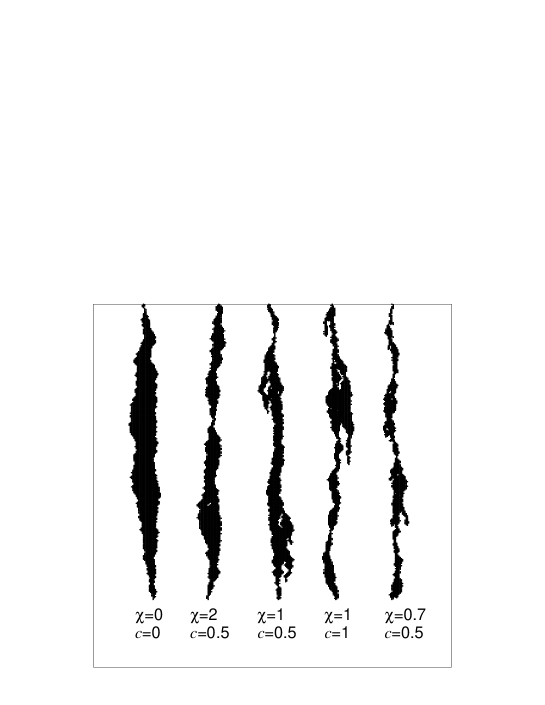
Figure 2: Snapshot of five avalanches for various values of $\chi$ and $c$. In all cases the avalanche duration is $t=500$. In order to display the details the avalanches are stretched by the factor 2 in the horizontal direction.

$ii)$ For $\chi<1$, the disorder is relevant, and leads to loss of criticality in the system. ${\cal{P}}_{t}$ tends to zero as $\exp{(-Kt^{1-\chi})}$, where $K$ is a constant which depends on $\chi$ and $c$. Thus the function $\overline{G}$ decreases to zero with the distance as a stretched exponential. In contrast to the case $\chi>1$ the avalanche propagation for $\chi<1$ is characterized by many branchings, though only one branch survives for long (see Fig. 2).

$iii)$ For $\chi=1$, the disorder is marginal and the avalanche distribution exponent varies continuously with the parameter $c$. Here, ${\cal{P}}_{t}$ tends to zero for large $t$ as $t^{-c}$. From Eq. (8), we see that $\overline{G}$ decreases as $t^{-1/2-c}$ and thus we find

$$\tau_{t}\;=\;\frac{3}{2}\,+\,c.$$ (12)

The avalanche distribution ${\rm Prob}\{duration\geq t\}$ still exhibits a power-law decay, but the exponent depends continuously on the amplitude $c$. This behavior has been verified in our simulations. Figure 3 displays the probability distribution ${\rm Prob}\{duration\geq t\}$ for three different values of $c$. For sufficiently large durations the asymptotic behavior agrees with Eq. (12).

Figure 3: The probability distribution ${\rm Prob}\{duration\geq t\}$ for $\chi=1$ and various values of $c$ for a system of size $L\times L$. The dashed lines correspond to the derived scaling behavior [Eq. (11)]. The probability distributions ${\rm Prob}\{duration\geq t\}$ are averaged over $50$ different representations of the disorder (hole-configuration) and $2\;10^{7}$ non-zero-avalanches for each disorder representation.

Let us now consider the distribution of masses of avalanches. We see from the explicit form of the avalanche propagator $\overline{G}$ that while its dependence on $t$ is modified by the disorder, its dependence on the transverse coordinate $x$ is unaffected. Hence, even in the presence of disorder, the average transverse size of an avalanche at depth $t$ scales as $t^{1/2}$. As each site in an avalanche topples only once, the average width of an avalanche cluster varies as $t^{1/2}$ and the total number of toppled sites $m$ scales as $t^{3/2}$. Then ${\rm Prob}\{mass\geq m\}\;\sim\;m^{-\tau_{m}+1}$ with

$$\tau_{m}\;=\;\frac{4}{3}\,+\,\frac{2}{3}\,c.$$ (13)

In our simulations, we used lattices of size $L\times T$ with $T=L$. In this case, the transverse size is effectively infinite as even the largest avalanches are not affected by the finite transverse size. Thus the finite-size effects are governed by the longitudinal size ($T$) alone, and the mass distribution is expected to fulfill the finite-size scaling ansatz [16]

$${\rm Prob}(mass\geq m|T)\sim\;T^{-\beta}\,f(T^{-\nu}m).$$ (14)

If finite-size scaling works a data collapse of the distributions for different system sizes $L\times T$ (with $L=T$) is obtained for $\nu=3/2$ and $\beta=1/2+c$. The corresponding scaling plots for three different values of $c$ are shown in Fig. 4. In all cases we observed good data collapse which confirms the above analysis.

Figure 4: Finite-size scaling analysis of the mass probability distribution ${\rm Prob}\{mass\geq m\}$ for $\chi=1$, three different values of $c$ and for various system sizes $L\in\{256,512,...,8192\}$. To avoid an overlap the curves for $c=0.5$ and $c=0.25$ are shifted in the lower-left direction.

4 The three-point correlation function

In the previous section we obtained the avalanche exponents by using some scaling arguments, which are not careful in distinguishing the probability that a given site at depth $t$ is toppled in an avalanche from the probability that at least one site at depth $t$ is toppled. We now present a cleaner derivation of the above results.

Let us denote the number of sites toppling in the layer $t$ by $N(t)$. Based on the experience with the model without disorder, we make the assumption that the distribution of avalanches in this model can be described by the scaling function

$$P(N(t)=n)\;\sim\;A\,t^{-a}\,{\cal F}(n/t^{b})$$ (15)

for $n\neq 0$ and where the scaling function ${\cal F}(x)$ decreases fast for large $x$, and $A$ is a constant. From this scaling form, it follows that $\langle N(t)\rangle\sim t^{2b-a}$, and $\langle N^{2}(t)\rangle\sim t^{3b-a}$. Thus knowing the $t$-dependence of $\langle N(t)\rangle$ and $\langle N^{2}(t)\rangle$, we can determine the exponents $a$ and $b$. Clearly, using Eq.(8) we get

$$\langle N(t)\rangle\;=\;\sum_{x}\;\overline{G}(x,t|0,0)=\;\frac{1}{2}\;{\cal{P}}_{t}.$$ (16)

We would now like to calculate $\langle N^{2}(t)\rangle$. Let $\overline{G}^{(3)}(x_{1},x_{2},t)$ be the probability that both sites $x_{1}$ and $x_{2}$ at depth $t$ topple when a particle is added at $x=0$ on the top layer $t=0$, averaged over all configurations of the disorder. Then, clearly, we have

$$\langle N^{2}(t)\rangle\;=\;\sum_{x_{1}}\sum_{x_{2}}\,\overline{G}^{(3)}(x_{1},x_{2},t).$$ (17)

For $t>0$, the three-point correlation function $\overline{G}^{(3)}$ satisfies the equation

$$\overline{G}^{(3)}(x_{1},x_{2},t)=(1-f_{t})^{2}\sum_{e_{1},e_{2}=\pm 1}\,\frac{1}{4}\,\overline{G}^{(3)}(x_{1}+e_{1},x_{2}+e_{2},t-1)$$ (18)

for $x_{1}\neq x_{2}$. We have to supplement this equation with the boundary condition for $x_{1}=x_{2}$:

$$\overline{G}^{(3)}(x_{1},x_{1},t)=\overline{G}(x_{1},t).$$ (19)

As for the case with no disorder, Eq.(18) is solved by the ansatz

$$\overline{G}^{(3)}(x_{1},x_{2},t)=\sum_{u=0}^{t}\sum_{y}\,f(y,u)\,\overline{G}(x_{1},t|y,u)\,\overline{G}(x_{2},t|y,u)$$ (20)

which satisfies Eq.(18) automatically for $x_{1}\neq x_{2}$. We choose the function $f(y,u)$ so that the equation holds also if $x_{1}=x_{2}$. Putting $x_{1}=x_{2}=x$ in the previous equation, we get

$$\overline{G}(x,t)=\sum_{u=0}^{t}\sum_{y}\,f(y,u)\,\overline{G}^{2}(x,t|y,u)$$ (21)

This is a linear equation connecting $f(y,u)$ to its values at sites higher up. Hence these can be solved recursively. The calculation of $\langle N^{2}(t)\rangle$ can be further simplified. We define the function

$$F(u)=\sum_{y}f(y,u),$$ (22)

and note that

$$\sum_{x}\overline{G}(x,t|y,u)={\frac{1}{2}}\,{\cal{P}}_{t}\,/\,{\cal{P}}_{u-1},$$ (23)

where we define ${\cal{P}}_{-1}=1$. Then using Eqs.(17,20), we get

$$\langle N^{2}(t)\rangle=\frac{1}{4}\,{\cal P}_{t}^{2}\,\sum_{u=0}^{t}\;{\cal{P}}_{u-1}^{-2}\,F(u).$$ (24)

The recursion equation for $F(u)$ is also easily deduced from the recursion equation for the function $f(y,u)$. We note that $\sum_{x}\overline{G}^{2}(x,t|y,u)$ is independent of $y$ and only depends on $t$ and $u$. Let us write

$$\sum_{x}\overline{G}^{2}(x,t|y,u)=K(t,u).$$ (25)

Then summing Eq.(21) over $x$, we get

$${\frac{1}{2}}\,{\cal{P}}_{t}=\sum_{u=0}^{t}\,F(u)\,K(t,u).$$ (26)

The effect of the disorder is just to introduce an overall rescaling factor to $K(t,u)$ in the absence of disorder:

$$K(t,u)={\cal{P}}_{t}^{2}\,{\cal{P}}_{u-1}^{-2}\;\sum_{x}\,G_{0}^{2}(x,t|y,u).$$ (27)

This implies that the asymptotic behavior of $F$ is given by

$$F(u)\sim u^{-c-1/2}.$$ (28)

Substituting in Eq.(24), we see that

$$\langle N^{2}(t)\rangle\;\sim\;t^{1/2-c}.$$ (29)

The obtained scaling behavior of $\langle N(t)\rangle$ and $\langle N^{2}(t)\rangle$ implies that the exponents of the assumed scaling form [Eq.(15)] are given by $a=1+c$, and $b=1/2$. This justifies the earlier heuristic calculation of the exponents.

It is straight-forward to extend this treatment to higher dimensions. We only mention the result here: in two (i.e. $2+1$ dimensions) and higher dimensions the avalanche exponents are given by

$$\tau_{t}\;=\;2\,+\,c,\quad\quad{\rm and}\quad\quad\tau_{m}\;=\;(3+c)/2.$$ (30)

As in the case with no disorder, there are logarithmic correction terms to the exponent values given above in the two-dimensional case.

5 Discussion

Let us comment briefly on the relationship of this model to that studied earlier by TD. Their stochastic variant of the directed sandpile model is defined on the same lattice as presented in Fig. 1, and particles are added on the top layer at random, and removed from below. The difference from the model studied here is that there is no quenched randomness, and the stochastic toppling rules are defined as follows: If a particle is added to a site, only then is the site examined for toppling. If the number of particles exceeds $2$, with a non-$1$ probability $p$ a toppling occurs and one particle is transferred to each of the two downward sites, and with probability $(1-p)$ nothing happens. While there is particle conservation in the TD model, so far as the evolution of a single avalanche is considered, the sites where no toppling occurs when particles are added, act as sink sites. The density of sink sites is higher near the top in both models. The randomness in the TD model provided by the stochastic toppling rules is ‘annealed’, unlike the quenched randomness in the model studied here.

In [10], it was shown that this model has a steady state for $p\geq p^{\star}$, where $p^{\star}$ is the critical probability for directed site percolation on a square lattice. In the steady state, there is a small fraction of sites having number of particles $2,3,4,\ldots$, but the average density is finite, and is a function of the depth of the layer.

TD argued that a density less than the bulk density locally corresponds to a finite correlation length which is spatially varying. They argued if the medium has an inverse correlation length $\kappa(t)$, which is small, and varies slowly as a function of $t$, then the survival probability of a disturbance up to depth $t$ is given by

$${\rm Prob}(t)\;\sim\;{\rm Prob}_{0}(t)\;\;\exp{\left(-\int_{0}^{t}\kappa(t^{\prime})dt^{\prime}\right)}.$$ (31)

The first factor is what we should get if $\kappa(t)$ is zero everywhere. The second term is a simple generalization of the $\exp{(-\kappa t)}$ factor when $\kappa(t)$ varies with $t$. We note that the expression is non-perturbative, in that the small parameter $\kappa$ is exponentiated. More importantly, $\kappa$ is usually a nontrivial power of the starting perturbation $\delta\rho(t)$ in the density (in the TD case, $\kappa(t)\sim[\delta\rho(t)]^{\nu}$, where $\nu$ is the longitudinal correlation length of directed percolation problem).

In the TD model, $\kappa(t^{\prime})$ varies as $c/t^{\prime}$, and hence the argument of the exponential varies as $-c\,\log{t}$, for large $t$. This immediately gives the $c$-dependence of the power-law behavior of ${\rm Prob}(t)$.

Using explicit calculation of correlation functions for small finite $t$, it is easy to verify that Eq. (31) is not exactly valid for the TD case. However, for the subsequent derivation the exponents of the TD model to be valid, the ansatz has to be at least asymptotically exact. As a proper treatment of the correlations in the steady state of TD model seems very difficult, one may try to find other simpler models where the validity of the ansatz can be demonstrated.

The steady state in our model is very simple, and thus the model is a good testing-ground. It is gratifying that, in the present model, the ansatz does become exact, and the two-point correlation function satisfies Eq. (8) exactly. Thus we have shown that this approximation is exact for our model.

The approximation is in the spirit of the familiar semiclassical Wentzel-Kramers-Brillouin-Jeffreys approximation in quantum mechanics [17]. We note that the mathematical mechanism giving rise to continuous variation of critical exponents with amplitude of perturbation applies to a much wider class of problems. Consider, for example, the generalization of the equilibrium problem treated in [8] involving extended surface defects to general $p$-vector spins $\{{\bf S}({\bf n})\}$ in $d$-dimensional half-space. Lattice sites are labelled by a $d$-dimensional integer vector ${\bf n}=(n_{1},n_{2},\ldots,n_{d})$ with $n_{1}>0$. The Hamiltonian of the system is

$${\mathcal{H}}=\sum J({\bf n,n^{\prime}})\,{\bf S}({\bf n})\cdot{\bf S}({\bf n^{\prime}})$$ (32)

where the summation is over all nearest neighbor pairs of sites ${\bf n,n^{\prime}}$. The coupling constant $J({\bf n,n^{\prime}})$ is assumed to depend only on $n_{1}$ (we may assume that $n_{1}\leq n_{1}^{\prime}$) as

$$J({\bf n,n^{\prime}})=J^{\star}-C\,n_{1}^{-\chi}$$ (33)

where $J^{\star}$ is the value of coupling in the bulk, and $C>0$.

As mentioned earlier, the simple renormalization argument due to Burkhardt [9] shows that for $\chi>1/\nu$, where $\nu$ is the (bulk) correlation length exponent, this perturbation is irrelevant, and for $\chi<1/\nu$, it is relevant. In the marginal case $\chi=1/\nu$, we get the inverse correlation length $\kappa(n_{1})\sim C^{\nu}/n_{1}$. Let us consider the spin-spin correlation function $\langle{\bf S}({\bf n})\cdot{\bf S}({\bf n^{\prime}})\rangle$. For simplicity, we may take ${\bf n}$ and ${\bf n^{\prime}}$ to differ only in the first coordinate. Then, it is easy to write an expression for this correlation function using the ansatz Eq. (31). The mathematical problem then is the same as discussed in this paper, and one finds that in the marginal case $\chi=1/\nu$, and the critical exponent corresponding to the decay of this correlation function varies linearly with $C^{\nu}$.

Of course, the dramatic effect of the boundary-perturbations on the exponents of the avalanche size distribution is due to the fact that all avalanches are initiated at the top boundary in our model. If we add particles at a fixed distance $t_{0}$ from the boundary, it is easy to see that large avalanches of duration much greater than $t_{0}$ have the same asymptotic behavior as the case $t_{0}=0$. However, shorter avalanches find significantly fewer defects than if they had been added at the top. If we added particles everywhere in the bulk, the avalanche size distribution is averaged over different values of $t_{0}$, and in the thermodynamical limit is the same as the case without defects.

We thank M. Barma for a critical reading of the manuscript. S. Lübeck would like to thank V. B. Priezzhev and A. Hucht for useful discussions.

References

- [1] For a general overview, see P. Bak, How nature works, (Springer, New York, 1996), H. J. Jensen, Self-Organized Criticality, (Cambridge University Press, Cambridge, 1998).
- [2] A well-studied example is the asymmetric diffusion of hard-core particles on a line. See for instance B. Derrida and M. R. Evans, in Nonequilibrium Statistical Mechanics in One Dimension, ed. by V. Privman, (Cambridge University Press, Cambridge, 1997), p. 277.
- [3] A review of surface critical phenomena may be found in F. Igloi, I. Peschel, and L. Turban, Adv. Phys. 42, 685 (1993).
- [4] P. Bak and C. Tang and K. Wiesenfeld, Phys. Rev. Lett. 59, 381 (1987).
- [5] J. G. Brankov, E. V. Ivashkevich and V. B. Priezzhev, J. Phys. (Paris) I 3, 1729 (1993).
- [6] A. A. Ali, Phys. Rev. E 52, R4595 (1995).
- [7] In the two-dimensional BTW model, there is some evidence that avalanches that reach the boundary have a different scaling behavior than avalanches that do not. [See, for example, C. Tebaldi, M. De Menech and A. L. Stella, Phys. Rev. Lett. 83, 3952 (1999)]. It seems plausible that the former will be affected by the power-law profile of the mean height near the surface.
- [8] H. J. Hilhorst and J. M. J. van Leeuwen, Phys. Rev. Lett., 47, 1188 (1981); T. W. Burkhardt, I. Guim, H. J. Hilhorst and J. M. J. van Leeuwen, Phys. Rev. B 30, 1486 (1984).
- [9] T. W. Burkhardt, Phys. Rev. Lett. 48, 216 (1982).
- [10] B. Tadić and D. Dhar, Phys. Rev. Lett. 79, 1519 (1997).
- [11] Directed stochastic models with multiple topplings (see e.g. R. Pastor-Satorras and A. Vespignani, J. Phys. A 33, L33 (2000); M. Paczuski and K. E. Bassler, e-print cond-mat/0005340; M. Kloster, S. Maslov and C. Tang, e-print cond-mat/0005528) belong to a different universality class.
- [12] D. Dhar and R. Ramaswamy, Phys. Rev. Lett. 63, 1659 (1989).
- [13] B. Tadić, U. Nowak, K. D. Usadel, R. Ramaswamy, and S. Padlewski, Phys. Rev. A 45, 8536 (1992).
- [14] J. Theiler, Phys. Rev. E 47, 733 (1993).
- [15] D. Dhar, Physica A 263, 4 (1999); a longer review is available at cond-mat/9909009.
- [16] L. P. Kadanoff, S. R. Nagel, L. Wu, and S. M. Zhou, Phys. Rev. A 39, 6524 (1989).
- [17] See, for example, P. M. Morse and H. Feshbach, Methods of Mathematical Physics, (McGraw-Hill, New York, 1953), p. 1092.