Quantum Coherence of the Ground State of a Mesoscopic Ring

Abstract

We discuss the phase coherence properties of a mesoscopic normal ring coupled to an electric environment via Coulomb interactions. This system can be mapped onto the Caldeira-Leggett model with a flux dependent tunneling amplitude. We show that depending on the strength of the coupling between the ring and the environment the free energy can be obtained either by a Bethe ansatz approach (for weak coupling) or by using a perturbative expression which we derive here (in the case of strong coupling). We demonstrate that the zero-point fluctuations of the environment can strongly suppress the persistent current of the ring below its value in the absence of the environment. This is an indication that the equilibrium fluctuations in the environment disturb the coherence of the wave functions in the ring. Moreover the influence of quantum fluctuations can induce symmetry breaking seen in the polarization of the ring and in the flux induced capacitance.

Pascal Cedraschi and Markus Büttiker

Quantum Coherence of the Ground State

1 Introduction

Mesoscopic physics is concerned with systems that are so small that the wave nature of the electrons becomes manifest. The quantum mechanical coherence properties of small electrical systems are thus a central topic of this field. In this work, we are interested in the coherence properties of the ground state of a mesoscopic system, namely a ring subject to an Aharonov-Bohm flux, which is capacitively coupled to an external environment which exhibits zero-point polarization fluctuations [1]. In a mesoscopic ring, quantum coherent electron motion leads, in the presence of an Aharonov-Bohm flux, to a ground state that supports a persistent current [2, 3, 4, 5, 6]. The persistent current is thus a signature of the coherence properties of the ground state of a mesoscopic ring. Only electrons whose wave function reaches around the ring contribute to the persistent current. Thermal fluctuations are known to reduce the amplitude of the persistent current [7, 8, 9]. On the other hand, the coherence properties of the ground state have thus far not been discussed. It is interesting to ask to what extent zero-point fluctuations of an electrical environment can influence the ground state of a ring, and how they affect the persistent current. This question is also interesting in view of the recent discussion on whether or not weak localization properties are influenced by zero-point fluctuations [10, 11, 12, 13, 14]. This discussion focuses on the conductance, a transport coefficient, and not directly on the ground state of the system. In this paper, we extend and clarify the results presented in [1]. A more intuitive discussion of the results of [1] based on a Langevin approach is given in [15]. Here we provide a detailed derivation based on Bethe ansatz results and perturbation theory of the results obtained in [1]. In addition, we investigate the capacitance coefficients of the ring and the charge-charge correlation spectrum. To be specific, we discuss the system shown in Fig. 1, namely a normal ring divided into two regions by tunnel barriers and coupled capacitively to an external electrical circuit. Each of the two regions can be described by a single potential, and the system considered permits thus a simple discussion of its polarizability.

Figure 1: Ring with an in-line dot subject to a flux $\Phi$ and capacitively coupled to an external impedance $Z_{ext}$.

We turn our attention to the specific case where the external impedance $Z_{\mbox{\scriptsize\it ext}}(\omega)$ shows resistive behavior at low frequencies. We consider the model discussed in [1], namely an impedance modeled by a transmission line. We investigate the persistent current, the charge on the dot and the flux induced capacitance which is the response of the charge to a variation in the magnetic flux through the ring. We identify two different classes of ground states as a function of the coupling between the external circuit and the ring, namely a “Kondo” type ground state at weak coupling and a symmetry broken ground state at strong coupling. In order to understand better the different regimes, we discuss time dependent quantities, in particular the power spectrum of the charge fluctuations on the dot.

The case of a resistive external circuit is of particular importance since the ring-dot structure coupled to a resistance exhibits dephasing at finite temperatures [15]. In view of the recent controversy concerning the question of whether there is dephasing at zero temperature [10, 11, 13] or not [12, 14], it is interesting to ask what we can learn about the ground state of our simple system if it is coupled to a resistive external circuit. The case where the dot and the arm of the ring are in resonance has already been treated in [1]. Below, we fill in the details left out in the discussion presented there and extend it to other thermodynamic quantities as well as to the noise spectrum of the charge on the dot. The discussion of the latter is of a particular interest since it exhibits decay of the correlations with time in the ground state. Here we emphasize an approach which treats the entire system in a Hamiltonian fashion. A more intuitive description of this system based on a Langevin equation approach has been given elsewhere [15].

2 Resistive external circuit

We model the finite impedance $Z_{\mbox{\scriptsize\it ext}}$ in a Hamiltonian fashion, with the help of a transmission line with capacitance $C_{t}$ and impedance $L$, see Fig. 2 and Appendix A. The ohmic resistance generated by the transmission line is $R=Z_{\mbox{\scriptsize\it ext}}(\omega=0)=(L/C_{t})^{1/2}$. We denote the charge operators on the capacitors between the inductances by $\hat{Q}_{n}$ and introduce the conjugate phase operators $\hat{\phi}_{n}$ fulfilling the commutation relations

$$[\hat{\phi}_{m},\hat{Q}_{n}]=ie\delta_{mn}.$$ (1)

It is via these charges and phases that the external circuit couples to the ring. The charge on the dot is $\hat{Q}_{d}$. We define the parallel internal capacitance $C_{i}\equiv C_{L}+C_{R}$, the external series capacitance $C_{e}^{-1}\equiv C_{1}^{-1}+C_{2}^{-1}$ and the total capacitances $C\equiv C_{i}+C_{e}$ and $C_{0}^{-1}\equiv C_{i}^{-1}+C_{e}^{-1}$. Then the Hamiltonian including all electrical interactions in the circuit reads, see Appendix A,

$$\hat{H}_{C}={\hat{Q}_{d}^{2}\over 2C_{i}}+{\hat{Q}_{d}\hat{Q}_{0}\over C_{i}}+{\hat{Q}_{0}^{2}\over 2C_{0}}+\hat{H}_{HO},$$ (2)

where $\hat{H}_{HO}$ is the Hamiltonian of a bath of harmonic oscillators describing the transmission line,

$$\hat{H}_{HO}=\sum_{n=1}^{\infty}\left\{{\hat{Q}_{n}^{2}\over 2C_{t}}+\left({\hbar\over e}\right)^{2}{(\hat{\phi}_{n}-\hat{\phi}_{n-1})^{2}\over 2L}\right\}.$$ (3)

The spectrum of $\hat{H}_{HO}$ is discussed in some detail in Appendix A. Here, we merely state that it is dense. Similar models involving a two-level system coupled to a bath of harmonic oscillators with a discrete set of fundamental frequencies are investigated in the context of stimulated photon emission. A known example is the Jaynes-Cummings model [16]. These models exhibit recurrence effects such as wave function revival [17, 18]. Because our model has a dense spectrum of fundamental frequencies of the harmonic oscillators, there are no recurrence phenomena [19].

Figure 2: Transmission line with impedance $Z_{ext}(\omega)=i\omega L/2+\sqrt{L/C_{t}-\omega^{2}L^{2}/4}$.

2.1 The total Hamiltonian

At low enough temperatures, we can describe the ring-dot system in terms of just two charge states, namely the state with $N$ electrons and the state with $N+1$ electrons in the dot. This leads to a two level system [20, 21] which we discuss briefly in Appendix B, and which is described by the Hamiltonian $\hat{S}\hat{H}_{e}^{\mbox{\scriptsize\it eff}}\hat{S}^{-1}$. The total Hamiltonian reads

$$\hat{H}^{\mbox{\scriptsize\it eff}}\equiv\hat{S}\hat{H}_{e}^{\mbox{\scriptsize\it eff}}\hat{S}^{-1}+\hat{H}_{C}={\hbar\varepsilon\over 2}\sigma_{z}-{\hbar\Delta_{0}\over 2}\sigma_{x}+{e\over 2C_{i}}\sigma_{z}\hat{Q}_{0}+\hat{H}_{HO}.$$ (4)

Let us briefly discuss the different terms of Eq. (4). The Pauli matrix $\sigma_{z}$ is related to the charge on the dot by $\hat{Q}_{d}=(e/2)\sigma_{z}+e(N-N_{+}+1/2)$, where $eN_{+}$ is an effective background charge. The detuning $\hbar\varepsilon$ is the energy difference that an electron must overcome if it wants to tunnel from the arm to the dot. It contains the one-particle energies $\epsilon_{d(N+1)}$ and $\epsilon_{aM}$, and a term stemming from the Coulomb interactions, Eq. (2). It reads

$$\hbar\varepsilon=\epsilon_{d(N+1)}-\epsilon_{aM}+{e^{2}\over C}\left(N-N_{+}+{1\over 2}\right).$$ (5)

The tunneling across the barriers between the dot and the arm is mediated by $\hbar\Delta_{0}\,\sigma_{x}/2$, where the tunneling amplitude $\hbar\Delta_{0}$ depends on the flux $\Phi$ and is given in Eq. (67). The term $(e/2C_{i})\sigma_{z}\hat{Q}_{0}$ is responsible for the capacitive coupling between the ring and the external circuit, whose Hamiltonian $\hat{H}_{HO}$ is given in Eq. (3).

The Hamiltonian $\hat{H}^{\mbox{\scriptsize\it eff}}$ given in Eq. (4) is the Caldeira-Leggett model [22, 19]. To make the connection to this model more explicit, we introduce the cut-off frequency $\omega_{c}=(LC_{t})^{-1/2}$ of the transmission line and the parameter $\alpha$ describing the strength of the coupling to the bath

$$\alpha\equiv{R\over R_{K}}\left({C_{0}\over C_{i}}\right)^{2},$$ (6)

where $R_{K}\equiv h/e^{2}$ denotes the quantum of resistance, and $R=(L/C_{t})^{1/2}$ is the zero-frequency impedance of the external circuit. The low energy behavior of a system described by the Hamiltonian of Eq. (4) is determined by the parameters $\alpha$, $\omega_{c}$, $\Delta_{0}$ and $\varepsilon$. The limit of a ring which is not coupled to an environment is recovered by setting $\alpha=0$. This limit corresponds to vanishing external capacitances, $C_{1}=C_{2}=0$, implying that $C_{0}=0$. Before discussing in more detail the different regimes associated with different values of those parameters, let us rewrite the coupling between the two level system and the bath in a form that is more suitable for our purposes.

We introduce the unitary transformation

$$\hat{U}=\exp\left(-{i\over 2}{C_{0}\over C_{i}}\hat{\phi}_{0}\sigma_{z}\right).$$ (7)

With this transformation, we define an equivalent Hamiltonian

$$\hat{H}\equiv\hat{U}\hat{H}^{\mbox{\it\scriptsize eff}}\hat{U}{}^{-1}.$$ (8)

A simple calculation yields $\hat{H}=\hat{H}_{TLS}+\hat{H}_{HO}+\hat{H}_{I}$, where $\hat{H}_{HO}$ has already been defined in Eq. (3), and

$$\hat{H}_{TLS} = {\hbar\varepsilon\over 2}\sigma_{z},$$ (9)

$$\hat{H}_{I} = -{\hbar\Delta_{0}\over 2}\left[\sigma_{+}\exp\left(i{C_{0}\over C_{i}}\hat{\phi}_{0}\right)+\sigma_{-}\exp\left(-i{C_{0}\over C_{i}}\hat{\phi}_{0}\right)\right].$$ (10)

The coupling between the ring and the external circuit is thus mediated by the operator $\exp[-i(C_{0}/C_{i})\hat{\phi}_{0}]$ which increases the charge on the capacitor $C_{1}$ (see Fig. 1) by $e\,C_{0}/C_{i}$. We emphasize that the charge on the capacitor $C_{1}$ is in general not shifted by an integer multiple of the electron charge when an electron tunnels between the dot and the arm of the ring. For a more thorough discussion, see Appendix C. We investigate the correlator

$$P(t)\equiv\left\langle\exp\left(i{C_{0}\over C_{i}}\hat{\phi}_{0}(t)\right)\exp\left(-i{C_{0}\over C_{i}}\hat{\phi}_{0}(0)\right)\right\rangle_{0},$$ (11)

in particular its long time behavior. Here, $\hat{\phi}_{0}(t)\equiv e^{i\hat{H}t/\hbar}\hat{\phi}_{0}e^{-i\hat{H}t/\hbar}$ is the time dependent phase operator, and $\langle\ldots\rangle_{0}$ denotes the expectation value taken with respect to the ground state for $\Delta_{0}=0$, see also Appendix D. It is shown in there that the correlator $P(t)$ behaves asymptotically like

$$P(\tau)\sim\left(1+i\omega_{c}|t|\right)^{2\alpha},\quad(t\to\infty).$$ (12)

Eq. (12) is of central importance. It allows to show that at $\alpha=1/2$ the problem can be mapped onto the exactly solvable Toulouse limit, Sec. 4.2. Moreover, it allows for a discussion of the thermodynamic properties of the problem using perturbation theory, see Sec. 3.2. Furthermore, the correlator $P(t)$ is closely related to the function $P(E)$ encountered in the discussion of tunneling through a tunnel barrier shunted by an impedance, see [23] and Appendix C. The discussion of $P(E)$ is generally referred to as “$P(E)$-theory”.

3 Ground state properties

In this section, we discuss ground state properties of the ring-dot structure coupled to a resistive external circuit. We are mainly interested in the persistent current. However, we also discuss two quantities related to the polarizability of the ring-dot structure, namely the charge on the dot, $\hat{Q}_{d}$ and the flux induced capacitance $C_{\Phi}$ [20, 21] which is the response of the charge on the dot to a variation in the magnetic flux $\Phi$, much in the same way as the electrochemical capacitance (see, for instance [24]) is the response of the charge to a variation in the applied bias.

3.1 Equivalent models

The anisotropic Kondo model, see e.g. [25], the resonant level model [26] and the inverse square one-dimensional Ising model [27] are equivalent to the Caldeira-Leggett model in their low energy properties. For vanishing magnetic field, corresponding to our model being at resonance $\varepsilon=0$, those models are characterized by two parameters, which may be identified as $\alpha$ and $\Delta_{0}/\omega_{c}$. The half plane spanned by $\Delta_{0}/\omega_{c}\geq 0$ and $\alpha$ is divided up into three regions by the separatrix equation $|1-\alpha|=\Delta_{0}/\omega_{c}$, where the parameters flow to different fixed points under the action of the renormalization group [28], see also Fig. 3. The regime of strong tunneling $\Delta_{0}/\omega_{c}>|1-\alpha|$ is beyond the scope of this work, and we shall not consider it any further. Of the remaining two, the region $\alpha>1$, $\Delta_{0}/\omega_{c}<\alpha-1$ corresponds to the ferromagnetic Kondo model where $\Delta_{0}/\omega_{c}$ renormalizes to zero, whereas the region $\alpha<1$, $\Delta_{0}/\omega_{c}<1-\alpha$ corresponds to the anti-ferromagnetic Kondo model that has been solved by Bethe ansatz [29, 30]. For large detuning $\varepsilon$, both cases can be treated by a perturbative expansion in $\Delta_{0}$. The details of this expansion are treated in Appendix D.

Figure 3: Scaling trajectories in the half plane spanned by $\alpha$ and the normalized tunneling amplitude $\Delta_{0}/\omega_{c}$. If the cut-off is lowered from $\omega_{c}$ to $\omega_{c}-d\omega_{c}$, scaling takes place along the lines in the direction of the arrows. The bold lines correspond to the separatrix equation $|1-\alpha|=\Delta_{0}/\omega_{c}$, dividing the plane up into the strong tunneling (S), the ferromagnetic (F) and the anti-ferromagnetic (AF) Kondo region. This diagram has been investigated by Anderson, Yuval, and Hamann [28].

3.2 Perturbative results

At zero temperature and to second order in $\Delta_{0}$, the free energy is $F_{0}+\delta F$ with (see Appendix D) $F_{0}=-\hbar|\varepsilon|/2$, and we find

$$\delta F=-{\hbar\omega_{c}\over 4}\left({\Delta_{0}\over\omega_{c}}\right)^{2}e^{|\varepsilon|/\omega_{c}}\left|{\varepsilon\over\omega_{c}}\right|^{2\alpha-1}\Gamma\left(1-2\alpha,{|\varepsilon|\over\omega_{c}}\right),$$ (13)

where $\Gamma(\zeta,x)$ is the incomplete gamma function. If the detuning $\varepsilon$ is large in magnitude, that is, far away from resonance, Eq. (13) is valid at any $\alpha$ up to second order in $\Delta_{0}/\omega_{c}$. In the regime $\alpha-1\gg\Delta_{0}/\omega_{c}$ (the ferromagnetic regime of the Kondo model, see Fig 3), Eq. (13) is valid even for arbitrary detuning $\varepsilon$. From Eq. (13), we easily obtain the persistent current in perturbation theory

$$I=-c{\partial\delta F\over\partial\Phi}=-{\hbar c\over 2}{\Delta_{0}\over\omega_{c}}{\partial\Delta_{0}\over\partial\Phi}e^{|\varepsilon|/\omega_{c}}\left|{\varepsilon\over\omega_{c}}\right|^{2\alpha-1}\Gamma\left(1-2\alpha,{|\varepsilon|\over\omega_{c}}\right).$$ (14)

Note that therefore for $\alpha>1$, where Eq. (14) is valid for arbitrary detuning, the persistent current has a cusp at resonance, see Fig. 4. It is well known [31, 32] that the Caldeira-Leggett model exhibits symmetry breaking for $\alpha>1$, namely $\langle\sigma_{z}\rangle=\partial F/\partial(\hbar\varepsilon)$ exhibits a finite jump as $\varepsilon$ crosses zero, see Fig. 5. By virtue of Eq. (68), $\langle\sigma_{z}\rangle$ is related to the average charge $\langle\hat{Q}_{d}\rangle$ on the dot. Let us briefly illustrate this relation. For $\varepsilon\to-\infty$, $\langle\sigma_{z}\rangle$ goes to $+1$, and the charge on the dot approaches therefore an integer multiple of the electron charge $e(N+1-N_{+})$. As $\varepsilon$ increases and goes towards zero, $\sigma_{z}$ approaches $0$ as well (unless there is symmetry breaking, in which case it approaches a finite positive value). At $\langle\sigma_{z}\rangle=0$, the charge on the dot is a half-integer multiple of the electron charge, $\langle\hat{Q}_{d}\rangle=e(N+1/2-N_{+})$, and for $\varepsilon\to+\infty$, the charge on the dot approaches again an integer multiple of $e$. In the following, we discuss for convenience the average $\langle\sigma_{z}\rangle$, bearing in mind that the physically more meaningful quantity is the charge on the dot $\langle\hat{Q}_{d}\rangle$.

Figure 4: The persistent current as a function of the normalized detuning $\varepsilon/\omega_{c}$ for $\alpha=0$ (solid line), $\alpha=1/2$ (dotted line) and $\alpha=1.2$ (dashed line). Units are chosen such that the persistent current for $\alpha=0$ is unity at resonance $\varepsilon=0$. Note the different scale for the persistent current at $\alpha=1.2$. The parameters are $\omega_{c}=10\Delta_{0}$.

The average $\langle\sigma_{z}\rangle$ is an odd function of $\varepsilon$, and for $\varepsilon>0$ it reads in perturbation theory

$$\left\langle\sigma_{z}\right\rangle = -{1\over 2}+{1\over 4}\left({\Delta_{0}\over\omega_{c}}\right)^{2}e^{\varepsilon/\omega_{c}}\Bigg{\{}\sum_{n=0}^{\infty}{(-1)^{n}\over n!}{(\varepsilon/\omega_{c})^{n}\over(1-2\alpha+n)(2-2\alpha+n)}$$ (15)

$$- \Gamma(1-2\alpha)\left({\varepsilon\over\omega_{c}}\right)^{2\alpha-2}\left[{\varepsilon\over\omega_{c}}+2\alpha-1\right]\Bigg{\}},$$

where we have used the series expansion for the incomplete gamma function, see Eq. (105). In the case of symmetry breaking, $\alpha>1$, the width of the jump at $\varepsilon=0$ is thus

$$\langle\sigma_{z}\rangle_{\varepsilon=0-}-\langle\sigma_{z}\rangle_{\varepsilon=0+}=1-\left({\Delta_{0}\over\omega_{c}}\right)^{2}{1\over 2(2\alpha-1)(2\alpha-2)},$$ (16)

see also Fig. 5. The jump in $\langle\sigma_{z}\rangle$ and the cusp in the persistent current have the same origin, thus the cusp is an indicator of symmetry breaking.

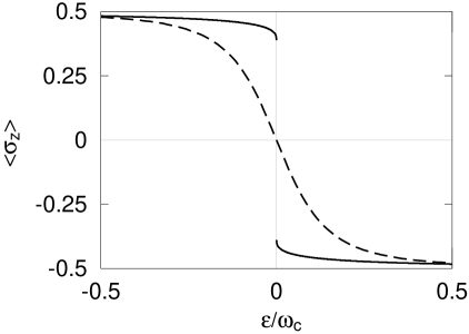
Figure 5: The position $\langle\sigma_{z}\rangle$ of the electron for $\alpha=1.2$ (solid line) showing symmetry breaking, compared to the typical behavior of $\langle\sigma_{z}\rangle$ at $\alpha=0$ (dashed line). The tunneling amplitude $\Delta_{0}/\omega_{c}=0.5$ is chosen very large in order to make the bending near $\varepsilon=0$ visible in the case of symmetry breaking.

The sensitivity of the charge $\langle\hat{Q}_{d}\rangle$ on the dot, see also Eq. (68), to changes in the magnetic flux $\Phi$ can be characterized in terms of the flux induced capacitance [21, 20]

$$C_{\Phi}\equiv{\partial\langle\hat{Q}_{d}\rangle\over\partial\Phi}=e{\partial\langle\sigma_{z}\rangle\over\partial\Phi},$$ (17)

It is an odd function of $\varepsilon$ as well, and for $\varepsilon>0$, it reads

$$C_{\Phi} = {e\over 2}{\Delta_{0}\over\omega_{c}}{\partial(\Delta_{0}/\omega_{c})\over\partial\Phi}e^{\varepsilon/\omega_{c}}\Bigg{\{}\sum_{n=0}^{\infty}{(-1)^{n}\over n!}{(\varepsilon/\omega_{c})^{n}\over(1-2\alpha+n)(2-2\alpha+n)}$$ (18)

$$- \Gamma(1-2\alpha)\left({\varepsilon\over\omega_{c}}\right)^{2\alpha-2}\left[{\varepsilon\over\omega_{c}}+2\alpha-1\right]\Bigg{\}}.$$

Like the average electron number, Eq. (16), it exhibits a finite jump at resonance

$$C_{\Phi}(\varepsilon=0+)-C_{\Phi}(\varepsilon=0-)=e{\Delta_{0}\over\omega_{c}}{\partial(\Delta_{0}/\omega_{c})\over\partial\Phi}{1\over(2\alpha-1)(2\alpha-2)},$$ (19)

for $\alpha-1\gg\Delta_{0}/\omega_{c}$. Thus the symmetry breaking can be seen as well in the flux induced capacitance, see Fig. 6. Flux sensitive screening in rings has recently been observed by Deblock et al. [6].

3.3 Bethe ansatz results

For $0<\alpha<1$, we use the Bethe ansatz solution of the resonant level model [33]. The low energy properties of the problem depend on three energy scales, namely the detuning $\varepsilon$, a cut-off $D$ and the “Kondo temperature”

$$T_{K}=\Delta_{0}\left({\Delta_{0}\over D}\right)^{\alpha\over 1-\alpha},$$ (20)

which is the only scale that depends on the magnetic flux $\Phi$. The persistent current is calculated from the known expression [33] for $\langle\sigma_{z}\rangle=\partial F/\partial(\hbar\varepsilon)$

$$\left\langle\sigma_{z}\right\rangle={i\over 4\pi^{3/2}}\int_{-\infty}^{\infty}{dp\over p-i0}e^{ip(\ln z+b)}{\Gamma(1+ip)\Gamma(1/2-i(1-\alpha)p)\over\Gamma(1+i\alpha p)},$$ (21)

where $z=(\varepsilon/T_{K})^{2(1-\alpha)}$ and $b=\alpha\ln\alpha+(1-\alpha)\ln(1-\alpha)$. This Bethe ansatz solution is valid for $1-\alpha>\Delta_{0}/\omega_{c}$. Now, we make use of the fact that in terms of the above-mentioned energy scales, and at zero temperature, the free energy reads $F=\hbar T_{K}f(\varepsilon/T_{K},T_{K}/D)$, where $f$ is a universal function. The persistent current $I=-c(\partial F/\partial\Phi)$ may thus be expressed in terms of $\langle\sigma_{z}\rangle=\partial F/\partial(\hbar\varepsilon)$

$$I=-\hbar c{\partial T_{K}\over\partial\Phi}\left[\int_{0}^{y}dx\,\langle\sigma_{z}\rangle(x)-y\langle\sigma_{z}\rangle(y)\right]+I_{0}.$$ (22)

where $y\equiv\varepsilon/T_{K}$. The integration constant $I_{0}$ is just the persistent current at resonance $\varepsilon=0$ and is determined below. The integral in Eq. (22) can be performed giving

$$I = {\hbar c\over\sqrt{\pi}}\left({\Delta_{0}\over\omega_{c}}\right)^{\alpha\over 1-\alpha}{\partial\Delta_{0}\over\partial\Phi}$$ (23)

$$\times \Bigg{\{}\sum_{n=1}^{\infty}{(-1)^{n}\over(n-1)!}{\Gamma\left({1\over 2}+n(1-\alpha)\right)e^{-nb}\over(1-2n(1-\alpha))\Gamma(1-n\alpha)}\left({\varepsilon\over T_{K}}\right)^{1-2n(1-\alpha)}$$

$$- {\Gamma\left(1-{1\over 2(1-\alpha)}\right)e^{-{b\over 2(1-\alpha)}}\over 2(1-\alpha)\Gamma\left(1-{\alpha\over 2(1-\alpha)}\right)}\Bigg{\}}+I_{0},$$

for $\ln z>-b$. Near resonance, more precisely for $\ln z<-b$, it reads

$$I = {\hbar c\over\sqrt{\pi}}{1\over 2(1-\alpha)}\left({\Delta_{0}\over\omega_{c}}\right)^{\alpha\over 1-\alpha}{\partial\Delta_{0}\over\partial\Phi}$$ (24)

$$\times \sum_{n=1}^{\infty}{(-1)^{n}\over n!}{\Gamma\left(1+{n-1/2\over 1-\alpha}\right)e^{{n-1/2\over 1-\alpha}b}\over\Gamma\left(1+(n-1/2){\alpha\over 1-\alpha}\right)}\left({\varepsilon\over T_{K}}\right)^{2n}+I_{0}.$$

For $\alpha=1/2$, the series in Eq. (24) can be explicitly re-summed

$$I\left(\alpha={1\over 2}\right)={\hbar c\over 16}{\Delta_{0}\over\omega_{c}}{\partial\Delta_{0}\over\partial\Phi}\ln\left[1+\left({16\over\pi}{\omega_{c}\over\Delta_{0}}{\varepsilon\over\Delta_{0}}\right)^{2}\right]+I_{0}.$$ (25)

This reflects the fact that the case $\alpha=1/2$ corresponds to an exactly solvable limit of the Kondo model, the Toulouse limit [34], see also Sec. 4.2. It remains to calculate the persistent current at resonance, $I_{0}$. We do so in the following paragraph.

We point out that $T_{K}$ sets the scale for the transition from resonant to perturbative behavior, i.e. for $|\varepsilon|\gg T_{K}$, the expressions for the persistent current from Bethe ansatz and from the perturbation theory must coincide up to terms of order $\Delta_{0}$. This observation allows us to determine the cut-off $D$ in terms of $\omega_{c}$,

$$\left({D\over\omega_{c}}\right)^{2\alpha}={2\Gamma(3/2-\alpha)e^{-b}\over\sqrt{\pi}(1-2\alpha)\Gamma(1-2\alpha)\Gamma(1-\alpha)},$$ (26)

as well as the integration constant $I_{0}$

$$I_{0}=-{\hbar c\over 2}{\Gamma(1-{1\over 2(1-\alpha)})e^{-{b\over 2(1-\alpha)}}\over\sqrt{\pi}(1-\alpha)\Gamma(1-{\alpha\over 2(1-\alpha)})}\left({\Delta_{0}\over D}\right)^{\alpha\over 1-\alpha}{\partial\Delta_{0}\over\partial\Phi}+{\hbar c\over 2}{1\over 1-2\alpha}{\Delta_{0}\over\omega_{c}}{\partial\Delta_{0}\over\partial\Phi}.$$ (27)

For $\alpha<1/2$, the first term in Eq. (27), behaving like $(\Delta_{0}/D)^{\alpha/(1-\alpha)}$ is dominating. For $\alpha>1/2$ the second one dominates and behaves as $\Delta_{0}/D$. The power law for $\alpha>1/2$ is thus the same as one obtains from perturbation theory at $\alpha>1$, using $I=-c\,\partial F/\partial\Phi$ with $F$ given by Eq. (13). The transition from the anti-ferromagnetic to the ferromagnetic Kondo model as $\alpha$ crosses 1 is therefore not seen in the persistent current at resonance, although it is visible, as stated above, as a cusp at resonance when the persistent current is traced as function of the detuning $\varepsilon$.

Leggett et al. [19] investigate coherence properties by discussing the decay of a state which is prepared such that the electron is e.g. in the dot for negative times $t<0$ (by applying a large negative detuning $\varepsilon$, for example) and released at $t=0$ (by setting $\varepsilon=0$ for $t\geq 0$). They find a decay with superimposed oscillations for $\alpha<1/2$ and a decay without oscillations for $\alpha>1/2$. This behavior is interpreted as decoherence setting in at $\alpha=1/2$. See also our discussion of the charge correlator in Sec. 4.

The persistent current, however, remains differentiable in $\varepsilon$ as $\alpha$ passes through $1/2$ and the ground state retains some coherence even for large $\alpha$, see also Sec. 4. As a function of detuning the cusp at resonance shows up only at $\alpha>1$. The poles at $\alpha=1/2$ in the two terms in Eq. (27) cancel each other. Together they give rise to a logarithmic persistent current

$$I_{0}\left(\alpha={1\over 2}\right)\approx\hbar c{\partial\Delta_{0}\over\partial\Phi}{\Delta_{0}\over\omega_{c}}\left(\ln{\Delta_{0}\over\omega_{c}}-0.217\ldots\right).$$ (28)

The logarithmic term $\ln(\Delta_{0}/\omega_{c})$ characterizes the transition from power law to linear behavior. The poles in the first term in Eq. (27) appearing at $\alpha=(2n+1)/(2n+2)$ for $n\geq 0$ are canceled by terms of higher order in $\Delta_{0}$.

The flux induced capacitance $C_{\Phi}$, see Sec. 3.2, can be obtained directly from the Bethe ansatz expression Eq. (21), giving for $\varepsilon>0$

$$C_{\Phi}={e\over\sqrt{\pi}}{\partial\Delta_{0}/\partial\Phi\over\Delta_{0}}\sum_{n=1}^{\infty}{(-1)^{n-1}\over(n-1)!}{\Gamma({1\over 2}+n(1-\alpha))e^{-nb}\over\Gamma(1-n\alpha)}\left({\varepsilon\over T_{K}}\right)^{-2n(1-\alpha)},\quad$$ (29)

for $\ln z>-b$, where $z$ and $b$ have been defined below Eq. (21). For $\ln z<-b$, it reads

$$C_{\Phi}={e\over\sqrt{\pi}(1-\alpha)}{\partial\Delta_{0}/\partial\Phi\over\Delta_{0}}\sum_{n=0}^{\infty}{(-1)^{n}\over n!}{\Gamma(1+{n+1/2\over 1-\alpha})e^{{n+1/2\over 1-\alpha}b}\over\Gamma(1+(n+1/2){\alpha\over 1-\alpha})}\left({\varepsilon\over T_{K}}\right)^{2n+1}.$$ (30)

There is no symmetry breaking for $\alpha<1$, that is $C_{\Phi}=0$ at resonance, see Fig. 6.

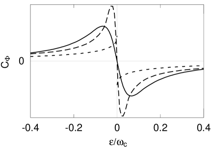
Figure 6: The flux induced capacitance as a function of the detuning $\varepsilon/\omega_{c}$ and for a tunneling amplitude $\Delta_{0}/\omega_{c}=0.2$. The flux induced capacitance is divided by $\partial\Delta_{0}/\partial\Phi$ such that the graph is independent of the flux $\Phi$, and given in arbitrary units. The solid line stands for $C_{\Phi}$ at $\alpha=0.3$, the long dashed line is $C_{\Phi}$ for $\alpha=0.6$. The short dashed line represents $C_{\Phi}$ at $\alpha=1.2$ blown up by a factor $5$ and exhibits symmetry breaking in $\varepsilon=0$.

4 Charge correlations

In this section, we consider charge-charge correlations on the dot at unequal times. These correlations may serve as an alternative measure of the coherence properties of the ground state. We define operator $\Delta\hat{Q}_{d}(t)$ of the charge fluctuations on the dot by

$$\Delta\hat{Q}_{d}(t)\equiv\hat{Q}_{d}(t)-\langle\hat{Q}_{d}\rangle,$$ (31)

where the time evolution of the operator $\hat{Q}_{d}$ is given by

$$\hat{Q}_{d}(t)\equiv e^{i\hat{H}t/\hbar}\hat{Q}_{d}e^{-i\hat{H}t/\hbar}.$$ (32)

With Eq. (68) the symmetrized charge correlations may be written in terms of the Pauli matrix $\sigma_{z}$

$$S_{QQ}(t)\equiv{1\over 2}\left\langle\left\{\Delta\hat{Q}_{d}(t),\Delta\hat{Q}_{d}(0)\right\}\right\rangle={e^{2}\over 8}\left(\left\langle\left\{\sigma_{z}(t),\sigma_{z}(0)\right\}\right\rangle-2\left\langle\sigma_{z}\right\rangle^{2}\right),\quad$$ (33)

where the curly brackets $\{\cdot,\cdot\}$ denote the anti-commutator $\{\hat{A},\hat{B}\}=\hat{A}\hat{B}+\hat{B}\hat{A}$. In the following we will concentrate on two simple cases, namely $\alpha=0$ and $\alpha=1/2$.

4.1 Correlations at $\alpha=0$

The case $\alpha=0$ is very easy to treat. In this case the ring is not coupled to the external circuit, and it suffices to calculate the charge correlator, Eq. (33) for the ground state of the $2\times 2$-matrix $(\hbar\varepsilon/2)\sigma_{z}-(\hbar\Delta_{0}/2)\sigma_{x}$, see Eq. (4), and we find

$$S_{QQ}(t)={e^{2}\over 4}{\Delta_{0}^{2}\over\varepsilon^{2}+\Delta_{0}^{2}}\cos\left(t\sqrt{\varepsilon^{2}+\Delta_{0}^{2}}\right).$$ (34)

The correlations are periodically oscillating with time, and the envelope of the oscillations is a constant. The spectral density $S_{QQ}(\omega)$, defined by

$$S_{QQ}(\omega)\equiv\int dt\,e^{i\omega t}S_{QQ}(t),$$ (35)

shows $\delta$-peaks at $\omega=\pm\sqrt{\varepsilon^{2}+\Delta_{0}^{2}}$

$$S_{QQ}(\omega)=\pi{e^{2}\over 4}{\Delta_{0}^{2}\over\varepsilon^{2}+\Delta_{0}^{2}}\left[\delta(\omega-\sqrt{\varepsilon^{2}+\Delta_{0}^{2}})+\delta(\omega+\sqrt{\varepsilon^{2}+\Delta_{0}^{2}})\right].$$ (36)

This also reflects the fact that there is no decay of the correlator with time.

4.2 Correlations at $\alpha=1/2$

In this section, we set $\hbar=1$. In the case $\alpha=1/2$ the Caldeira-Leggett model can be mapped on an exactly solvable limit of the Kondo model, the Toulouse limit [34]. Its Hamiltonian describes the hybridization of a continuum of spinless electrons with a localized electronic level but without electron-electron interactions. This can also be seen from the correlator $P(t)$, see Eq. (12), which for $\alpha=1/2$ takes the form

$$P_{\alpha=1/2}(t)\sim{1\over 1+i\omega_{c}|t|},\quad(t\to\infty).$$ (37)

This expression corresponds to the sum over all energies of the Green’s functions of free electrons in a symmetric wide band with linear dispersion and a density of states $dn/d\omega=\omega_{c}^{-1}$. We denote the spectrum of the electrons in the continuum by $\omega_{n}$ and their creation and annihilation operators by $\hat{b}_{n}^{\dagger}$ and $\hat{b}_{n}$, resp. The energy of the localized level is $\epsilon$ and its creation and annihilation operators are $\hat{c}^{\dagger}$ and $\hat{c}$. The strength of the hybridization is $J_{\pm}$. The Toulouse Hamiltonian then reads

$$\hat{H}_{\mbox{\scriptsize Toul}}=\int dn\,\omega_{n}\hat{b}_{n}^{\dagger}\hat{b}_{n}+\epsilon\,\hat{c}^{\dagger}\hat{c}+{J_{\pm}\over 2}\int dn\,\left(\hat{c}^{\dagger}\hat{b}_{n}+\hat{b}_{n}^{\dagger}\hat{c}\right),$$ (38)

Then the Caldeira-Leggett model at $\alpha=1/2$ is mapped onto the Toulouse limit by identifying the parameters, see [19]

$$\varepsilon\, \leftrightarrow \,\epsilon$$ (39)

$$\Delta_{0}\, \leftrightarrow \,2^{-1/2}J_{\pm}.$$ (40)

Moreover, we identify the Pauli matrix $\sigma_{z}$ in the Caldeira-Leggett model with the operator for the occupation of the localized level

$${1\over 2}\sigma_{z}\leftrightarrow\hat{c}^{\dagger}\hat{c}-{1\over 2}.$$ (41)

The Green’s functions for this Hamiltonian can be calculated in closed form. In order to calculate the charge correlator, Eq. (33), we need the time ordered Green’s function of the localized electron level

$$G_{d}(t)=-i\left\langle{\rm T}\hat{c}(t)\hat{c}^{\dagger}(0)\right\rangle\equiv-i\left[\theta(t)\left\langle\hat{c}(t)\hat{c}^{\dagger}(0)\right\rangle-\theta(-t)\left\langle\hat{c}^{\dagger}(0)\hat{c}(t)\right\rangle\right],\quad$$ (42)

where $\theta(t)$ is the Heaviside step function. In Fourier space, it takes the form

$$G_{d}(\omega)=\int_{-\infty}^{\infty}{d\omega\over 2\pi}e^{-i\omega t}G_{d}(t)=\left[\omega-\epsilon+i0-\Sigma_{d}(\omega)\right]^{-1},$$ (43)

where the self-energy $\Sigma_{d}(\omega)$ reads

$$\Sigma_{d}(\omega)=-i{\pi\over 2\omega_{c}}\left({J_{\pm}\over 2}\right)^{2}{\rm sign}\,\omega\equiv-{i\Gamma\over 2}{\rm sign}\,\omega,$$ (44)

where ${\rm sign}\,\omega$ denotes the sign of $\omega$. We shall see below that $\Gamma$ is in fact the inverse decay time of the charge correlations. In terms of the parameters of the Caldeira-Leggett model, it reads

$$\Gamma={\pi\over 2}{\Delta_{0}^{2}\over\omega_{c}}.$$ (45)

Using Eqs. (33) and (41), and with the help of Wick’s theorem, we find the charge correlations for $\alpha=1/2$ to be

$$S_{QQ}(t)=e^{2}{\rm Re}\,\left[G_{d}(t)G_{d}(-t)\right].$$ (46)

A rather long but simple calculation yields the spectral density

$$S_{QQ}(\omega)=e^{2}{2\Gamma\over\omega^{2}+\Gamma^{2}}f(\omega),$$ (47)

with

$$f(\omega) = {1\over 4\pi}\left[\arctan\left({|\omega|-\varepsilon\over\Gamma/2}\right)+\arctan\left({|\omega|+\varepsilon\over\Gamma/2}\right)\right]$$ (48)

$$- {1\over 8\pi}{\Gamma\over\omega}\left[\ln{\varepsilon^{2}+(\Gamma/2)^{2}\over(\omega-\varepsilon)^{2}+(\Gamma/2)^{2}}+\ln{\varepsilon^{2}+(\Gamma/2)^{2}\over(\omega+\varepsilon)^{2}+(\Gamma/2)^{2}}\right].\quad$$

Let us discuss $S_{QQ}(t)$. We have, see also Fig. 7,

$$f(\omega)\to{1\over 4},\quad\mbox{for $\omega\gg\max\{\varepsilon,\Gamma\}$},$$ (49)

and the Fourier transform of $2\Gamma/(\varepsilon^{2}+\Gamma^{2})$ is simply $e^{-\Gamma|t|}$. Moreover, for $t\to 0$, the correlation function $S_{QQ}(t)$ approaches the integral of the spectral density

$$S_{QQ}(0)=\int_{-\infty}^{\infty}{d\omega\over 2\pi}S_{QQ}(\omega),$$ (50)

which, for symmetry reasons, must equal $1/4$ for $\varepsilon=0$. A sketch of $S_{QQ}(0)$ is given in Fig. 8. The correlation function thus reads for short times

$$S_{QQ}(t)\sim S_{QQ}(0)\,e^{-\Gamma|t|},\quad(|t|\ll\min\{\varepsilon^{-1},\Gamma^{-1}\}).$$ (51)

For long times, we use the stationary phase expansion and get

$$S_{QQ}(t)\sim-{e^{2}\over\pi}{(\Gamma/2)^{2}\over\left[\varepsilon^{2}+(\Gamma/2)^{2}\right]^{2}}t^{-2},\quad(t\to\infty).$$ (52)

Thus the correlations decay exponentially with rate $\Gamma$ at small times and algebraically for large times. Moreover, since $S_{QQ}(\omega=0)=0$, the integral of $S_{QQ}(t)$ over all times must vanish, therefore $S_{QQ}(t)$ takes negative values at intermediate times, see Fig. 9. For $\varepsilon\neq 0$ the correlations are still oscillatory in time.

We have discussed here only the cases $\alpha=0$ and $\alpha=1/2$ which correspond to no coupling at all between the ring and the electric circuit ($\alpha=0$), and a relatively strong coupling ($\alpha=1/2$). At $\alpha=0$, the charge correlation spectrum reveals simply the coherent charge oscillations between the dot and the arm with a sharp frequency. At $\alpha=1/2$, charge transfer still occurs, but it is now entirely characterized by the (flux-sensitive) relaxation rate $\Gamma$ and the detuning. Instead of the periodic charge transfer which exists for $\alpha=0$, the charge transfer has a much more stochastic character. Together with the results for the persistent current and the polarizability of the ring obtained in the previous section, the charge correlation spectrum, discussed here, provides an additional measure of the coherence properties of the ground state.

Figure 7: The function $f(\omega)$ describing the deviation of the spectral density $S_{QQ}(\omega)$ at $\alpha=1/2$ from the spectral density of an exponentially decaying correlator. The frequency $\omega$ is measured in units of $\Gamma$.

Figure 8: Instantaneous charge correlations as a function of $\varepsilon$, which is measured in units of $\Gamma$ at $\alpha=1/2$. The function is symmetric under $\varepsilon\to-\varepsilon$. The correlations $S_{QQ}(t=0)$ (denoted by $S(0)$ in the figure) are measured in units of the squared electron charge $e^{2}$.

Figure 9: Time dependence of the charge correlations $S_{QQ}(t)$ (denoted by $S(t)$ in the figure) for different values of $\varepsilon$ in units of the squared electron charge $e^{2}$ at $\alpha=1/2$. The line showing the exponential decay $1/4\,\exp(-\Gamma t)$ is given for comparison. For $\varepsilon\neq 0$ the correlator exhibits damped oscillations.

5 Conclusions

We have investigated a simple model of a mesoscopic normal ring coupled to an external electrical circuit. We have shown that the zero-point fluctuations of the external circuit influence measurable quantities like the persistent current $I$, the flux induced capacitance $C_{\Phi}$, and the polarization of the ring. The reduction of the persistent current as well as the onset of symmetry breaking, observed in the polarization and in the flux induced capacitance indicate that the coherence of the wave function in the ring is reduced by fluctuations in the external circuit. While such a suppression of quantum coherence is not too surprising at finite temperatures, we have demonstrated in the present paper that it persists even in the extreme quantum limit of zero temperature.

A The Hamiltonian of the transmission line In order to understand the dynamics of the bath of harmonic oscillators describing the transmission line shown in Fig. 2, we have to discuss its properties in some detail. Its impedance is of the form $Z_{\mbox{\scriptsize\it ext}}(\omega)=i\omega L/2+(L/C_{t}-\omega^{2}L^{2}/4)^{1/2}$, see e.g. [35]. This appendix is devoted to the discussion of the Hamiltonian of the transmission line and its eigenstates. We denote the charges on the capacitors between the inductances by $Q_{n}$ and the potentials by $V_{n}$, $n=0,1,2,\ldots$. The charge $Q_{0}$ plays a special role, see Fig. 1, because it is the charge sitting on the capacitor $C_{1}$; $V_{0}$ is the corresponding potential. Similarly, $Q_{\infty}$ and $V_{\infty}$ are the charge and the potential on the capacitor $C_{2}$. It is via these charges and potentials that the external circuit couples to the ring. Furthermore, we introduce the phases $\phi_{n}$, which satisfy the equations

$${d\phi_{n}\over dt}={e\over\hbar}\left(V_{n}-V_{\infty}\right).$$ (53)

The canonically conjugate variables to the charges $Q_{n}$ are not the phases $\phi_{n}$ but rather the generalized fluxes $(\hbar/e)\phi_{n}$. We choose the dimensionless quantities $\phi_{n}$ for later convenience. In terms of these variables the Hamiltonian of the transmission line reads

$$H_{HO}=\sum_{n=0}^{\infty}\left\{{Q_{n}^{2}\over 2C_{t}}+\left({\hbar\over e}\right)^{2}{(\phi_{n+1}-\phi_{n})^{2}\over 2L}\right\},$$ (54)

which is canonically quantized by replacing the charges and phases by operators $\hat{Q}_{n}$ and $\hat{\phi}_{n}$ and by imposing the commutation relations $[\hat{\phi}_{m},\hat{Q}_{n}]=ie\,\delta_{mn}$, giving Eq. (3). We note that $Q_{n}$ plays the role of a momentum, and $\phi_{n}$ plays the role of a position. In particular, the quadratic form involving the charge $Q_{n}$ is positive definite. Due to a theorem of linear algebra, any pair of quadratic forms, one of which is positive definite, can be simultaneously diagonalized. Therefore, the Hamiltonian $\hat{H}_{HO}$ of Eq. (3) can be diagonalized by a unitary transformation mapping $\hat{Q}_{n}$ onto $\hat{Q}(x)$, and $\hat{\phi}_{n}$ onto $\hat{\phi}(x)$. The transformed operators $\hat{Q}(x)$ and $\hat{\phi}(x)$ satisfy the commutation relations $[\hat{\phi}(x),\hat{Q}(y)]=ie\,\delta(x-y)$. In this new basis $\hat{H}_{HO}$ reads

$$\hat{H}_{HO}=\int_{0}^{1}dx\,\left\{{\hat{Q}^{2}(x)\over 2C_{t}}+\left({\hbar\over e}\right)^{2}{2\over L}\sin^{2}\left({\pi x\over 2}\right)\hat{\phi}^{2}(x)\right\}.$$ (55)

In terms of the operators $\hat{Q}(x)$, the charge on the dot $\hat{Q}_{0}$ is given by

$$\hat{Q}_{0}=\sqrt{2}\int_{0}^{1}dx\,\cos\left({\pi x\over 2}\right)\hat{Q}(x),$$ (56)

and analogously, we have

$$\hat{\phi}_{0}=\sqrt{2}\int_{0}^{1}dx\,\cos\left({\pi x\over 2}\right)\hat{\phi}(x).$$ (57)

Eq. (57) will be useful in Appendix D in order to calculate the correlator $P(\tau)$. The diagonalized Hamiltonian Eq. (55), being a sum over harmonic oscillators, can be written in terms of the bosonic creation and annihilation operators $\hat{a}_{x}^{\dagger}$ and $\hat{a}_{x}$ which are related to the charges $\hat{Q}(x)$ and the phases $\hat{\phi}(x)$ by

$$\hat{\phi}(x) = {e\over i\hbar\sqrt{2\lambda_{x}}}\left(\hat{a}_{x}-\hat{a}_{x}^{\dagger}\right),$$ (58)

$$\hat{Q}(x) = \sqrt{\lambda_{x}\over 2}\left(\hat{a}_{x}+\hat{a}_{x}^{\dagger}\right),$$ (59)

with $\lambda_{x}=\hbar(C_{t}/L)^{1/2}\sin(\pi x/2)$, and which obey the commutation relations $[\hat{a}_{x},\hat{a}_{y}^{\dagger}]=\delta(x-y)$. In terms of the operators $\hat{a}_{x}$ and $\hat{a}_{x}^{\dagger}$, the Hamiltonian of the transmission line, Eq. (55) reads

$$\hat{H}_{HO}=\int_{0}^{1}dx\,\hbar\omega_{x}\left(\hat{a}_{x}^{\dagger}\hat{a}_{x}+{1\over 2}\right),$$ (60)

the eigenfrequencies $\omega_{x}$ being

$$\omega_{x}=\sqrt{1\over LC_{t}}\sin{\pi x\over 2}.$$ (61)

We note that the spectrum Eq. (61) is linear at low frequencies with a density of states $dx/d\omega\equiv(2/\pi)\omega_{c}^{-1}$, where $\omega_{c}=(LC_{t})^{-1/2}$, and that it is cut off at a frequency $\omega_{c}$. We shall need Eqs. (60) and (61) in Appendix D where we write the partition function of the Caldeira-Leggett model as a path integral.

B Degrees of freedom in the ring The Hamiltonian $\hat{H}_{C}$ of the Coulomb interactions, Eq. (2), has to be augmented by a Hamiltonian describing the electronic degrees of freedom inside the ring. We are interested in the effect of the long range nature of the Coulomb interactions, therefore we disregard charge redistribution and correlation effects and assume the potentials in the dot and the arm of the ring to be constant over the extent of the respective subsystem. As a consequence, the electronic wave functions are independent of the number of electrons in the dot and the arm. Moreover, we consider spinless electrons here. It has been demonstrated in [20, 21] that the inclusion of spin does not change the calculations a great deal although it somewhat changes the physics of the problem. In particular, the Kondo effect for an isolated ring sets in only for a tunneling amplitude $\hbar\Delta_{0}$ that is comparable to or larger than the mean level spacing in the dot or the arm, whereas in this paper we assume that $\hbar\Delta_{0}$ is much smaller than the mean level spacings. For a discussion of the Kondo effect in normal metal rings, see the articles of Eckle et al. [36] and of Kang and Shin [37]. We denote the creation operator for an electron of energy $\epsilon_{dj}$ in the dot by $\hat{d}_{j}^{\dagger}$ and the creation operator for an electron of energy $\epsilon_{ak}$ in the arm by $\hat{a}_{k}^{\dagger}$. The tunneling through the left barrier is described by a hopping amplitude $t_{jk}^{L}$, the tunneling through the right barrier by $t_{jk}^{R}$. The total tunneling amplitude includes the phase picked up by an electron whose wave function encloses the magnetic flux $\Phi$ and reads

$$t_{jk}(\Phi)\equiv t_{jk}^{L}+t_{jk}^{R}\exp\left(2\pi i{\Phi\over\Phi_{0}}\right).$$ (62)

where $\Phi_{0}=hc/e$ is the elementary flux quantum. As the dependence of the Hamiltonian on the magnetic field is shifted into the boundary conditions by Eq. (62), the tunneling amplitudes $t_{jk}^{L}$ and $t_{jk}^{R}$ can be taken to be real. Their relative sign depends on the number of nodes of the wavefunctions they couple. It is positive if the sum of the number of the nodes of the wavefunction in the dot with energy $\epsilon_{dj}$ and of the number of nodes of the wavefunction in the arm with energy $\epsilon_{ak}$ is even, and negative otherwise. This makes up for the parity effect in the persistent current. Now, we can write a noninteracting Hamiltonian for the electronic degrees of freedom

$$\hat{H}_{e}=\sum_{j}\epsilon_{dj}\hat{d}_{j}^{\dagger}\hat{d}_{j}+\sum_{k}\epsilon_{ak}\hat{a}_{k}^{\dagger}\hat{a}_{k}+\sum_{jk}\left[t_{jk}(\Phi)\hat{d}_{j}^{\dagger}\hat{a}_{k}+h.c.\right].$$ (63)

All the many-body interactions are taken into account by $\hat{H}_{C}$ of Eq. (2). The operator for the charge on the dot becomes

$$\hat{Q}_{d}=e\sum_{j}\hat{d}_{j}^{\dagger}\hat{d}_{j}-eN_{+},$$ (64)

with $eN_{+}$ being an effective background charge on the dot. Next, we make a crucial approximation, which allows us to write $\hat{H}_{e}$ and $\hat{Q}_{d}$ as $2\times 2$-matrices.

We shall assume in the following that the tunneling amplitudes through the left and the right barriers are much smaller in magnitude than the level spacing in the dot and the level spacing in the arm. We note that the number of charge carriers in the ring is conserved. Following Stafford and one of the authors [21, 20], we consider hybridization between the topmost occupied electron level in the arm and the lowest unoccupied electron level in the dot, $\epsilon_{aM}$ and $\epsilon_{d(N+1)}$ only. To simplify the notation, we denote the tunneling amplitudes between the levels $\epsilon_{aM}$ and $\epsilon_{d(N+1)}$ by $t_{L}$ for tunneling through the left barrier and by $t_{R}$ for tunneling through the right one, and we assume $t_{L}$ and $t_{R}$ to be positive. The Hamiltonian for the electronic degrees of freedom can be written in terms of the Pauli matrices $\sigma_{z}$ and $\sigma_{\pm}=(\sigma_{x}\pm i\sigma_{y})/2$

$$\hat{H}_{e}^{\mbox{\scriptsize\it eff}} = {\epsilon_{d(N+1)}-\epsilon_{aM}\over 2}\sigma_{z}-\left[t_{L}\pm t_{R}\exp\left(2\pi i{\Phi\over\Phi_{0}}\right)\right]\sigma_{+}$$ (65)

$$- \left[t_{L}\pm t_{R}\exp\left(-2\pi i{\Phi\over\Phi_{0}}\right)\right]\sigma_{-}+E_{0},$$

where $E_{0}=\sum_{j=1}^{N}\epsilon_{dj}+\sum_{k=1}^{M-1}\epsilon_{ak}+(\epsilon_{aM}+\epsilon_{d(N+1)})/2$. The terms in $\sigma_{\pm}$ describe the tunneling between the states $\epsilon_{d(N+1)}$ and $\epsilon_{aM}$. The relative sign of $t_{L}$ and $t_{R}$ is positive if the number $N+M$ of electrons in the ring is odd, and negative if it is even, as discussed in the previous paragraph. The unitary transformation $\hat{H}_{e}^{\mbox{\scriptsize\it eff}}\mapsto\hat{S}\hat{H}_{e}^{\mbox{\scriptsize\it eff}}\hat{S}^{-1}$ where $\hat{S}=\exp(-i\sigma_{z}\vartheta/2)$ and $\tan\vartheta=-t_{R}\sin(2\pi\Phi/\Phi_{0})/(t_{L}+t_{R}\cos(2\pi\Phi/\Phi_{0}))$, leaves the term in $\sigma_{z}$ unchanged and transforms the tunneling term as follows

$$\hat{S}\left\{\left[t_{L}\pm t_{R}e^{2\pi i\Phi/\Phi_{0}}\right]\sigma_{+}+\left[t_{L}\pm t_{R}e^{-2\pi i\Phi/\Phi_{0}}\right]\sigma_{-}\right\}\hat{S}^{-1}={\hbar\Delta_{0}\over 2}\sigma_{x},\quad\,$$ (66)

with

$${\hbar\Delta_{0}\over 2}=\sqrt{t_{L}^{2}+t_{R}^{2}\pm 2t_{L}t_{R}\cos\left(2\pi{\Phi\over\Phi_{0}}\right)},$$ (67)

the positive sign applying again for an odd number of electrons, the negative one for an even number of electrons in the structure. The charge on the dot, $\hat{Q}_{d}$, reads in the two level approximation

$$\hat{Q}_{d}={e\over 2}\sigma_{z}+e\left(N-N_{+}+{1\over 2}\right).$$ (68)

C Relation to $P(E)$-theory In this section we discuss the relation of the results obtained above to the “$P(E)$-theory” [23]. Usually, the $P(E)$-theory is employed in order to calculate the tunneling rate through a barrier which is shunted by an impedance $Z_{shunt}(\omega)$ in the Golden Rule approximation. The system discussed here is somewhat special in the sense that the impedance $Z_{ext}(\omega)$ does not act as a shunt, but is coupled only capacitively to the tunnel barrier, see Fig. 1. Therefore, the electrons in the ring cannot flow through the impedance as is the case for a shunt impedance. We can see the difference to ordinary $P(E)$-theory more clearly by considering the Hamiltonian $\hat{H}_{I}$, Eq. (10), responsible for the coupling between the ring and the transmission line. The operator $\exp[-i(C_{0}/C_{i})\hat{\phi}_{0}]$ appearing in Eq. (10) is a charge shift operator. It differs from the charge shift operator that is usually encountered in the context of tunneling in the $P(E)$-theory in that it does not change the charge on the capacitor $C_{1}$ by an integer multiple of the electron charge but by a fraction $(C_{0}/C_{i})e$,

$$e^{-i(C_{0}/C_{i})\hat{\phi}_{0}}\hat{Q}_{0}e^{i(C_{0}/C_{i})\hat{\phi}_{0}}=\hat{Q}_{0}-{C_{0}\over C_{i}}e.$$ (69)

The difference is due to the fact that the standard $P(E)$-theory does not consider $\hat{\phi}_{0}$ but an operator $\hat{\phi}$ which is canonically conjugate to the charge $\hat{Q}_{d}$ on the dot. This is no problem in an open system, where the conjugate operator $\hat{\phi}$ indeed exists. In our closed system with only two charge states, however, there is no conjugate operator to $\hat{Q}_{d}$, therefore we stick to the operator $\exp[i(C_{0}/C_{i})\hat{\phi}_{0}]$. The coupling to the external circuit modifies the tunneling such that the persistent current is reduced, as shown in the present paper. The modification is described by the correlator

$$K(t)\equiv\left({C_{0}\over C_{i}}\right)^{2}\left\langle\hat{\phi}_{0}(t)\hat{\phi}_{0}(0)-\hat{\phi}_{0}^{2}(0)\right\rangle_{0},$$ (70)

where $\langle\ldots\rangle_{0}$ denotes an expectation value with respect to the ground state for $\Delta_{0}=0$, see also Appendix D. The pre-factor $(C_{0}/C_{i})^{2}$ is characteristic for our problem and is due to the fact that we are considering the phase operator $\hat{\phi}_{0}$ of the external circuit. The correlator $K(t)$ is related to the function $P(t)$ given in Eq. (11) by $P(t)=\exp[K(t)]$, and the Fourier transform $P(E)$ of $P(t)$ has given the theory its name. For the purpose of calculations it is more convenient, however, to stay with the correlator $K(t)$. It has been mentioned above, see Eq. (12), that $K(t)\sim-2\alpha\ln(1+i\omega_{c}|t|)$ in the long time limit, where $\omega_{c}$ is the cut-off frequency, and $\alpha$ is identical to the coupling parameter given in Eq. (6), which determines the suppression of the persistent current, Eq. (27). In $P(E)$-theory, a general rule for calculating $K(t)$ at finite temperature is given,

$$K(t)=2\left({C_{0}\over C_{i}}\right)^{2}\int_{0}^{\infty}{d\omega\over\omega}{{\rm Re}\,Z_{ext}(\omega)\over R_{K}}\left(e^{-i\omega t}-1\right)\coth\left({\hbar\omega\over 2kT}\right).$$ (71)

In the zero temperature limit, this formula yields the same long time behavior as the one obtained above for a special realization of the transmission line.

D Thermodynamic properties of the Caldeira-Leggett model We want to write the Caldeira-Leggett Hamiltonian $\hat{H}=\hat{H}_{TLS}+\hat{H}_{HO}+\hat{H}_{I}$ in a form that is suitable for the path-integral formalism. For the bath of harmonic oscillators, described by $\hat{H}_{HO}$, this has been done in Eq. (60). The Hamiltonians containing the Pauli matrices $\sigma_{z}$ and $\sigma_{\pm}$ are translated into the operator formalism by introducing the fermion operators ${\hat{c}}^{\dagger}$, $\hat{c}$, creating and annihilating an electron the dot, and $\hat{\overline{c}}{}^{\dagger}$ and $\hat{\overline{c}}$, creating and annihilating an electron in the arm

$$\hat{H}^{\prime}_{TLS} = {\hbar\varepsilon\over 2}\left(\hat{c}^{\dagger}\hat{c}-\hat{\overline{c}}{}^{\dagger}\hat{\overline{c}}\right),$$ (72)

$$\hat{H}^{\prime}_{I} = -{\hbar\Delta_{0}\over 2}\left[\hat{c}^{\dagger}\hat{\overline{c}}\exp\left(i{C_{0}\over C_{i}}\hat{\phi}_{0}\right)+\hat{\overline{c}}{}^{\dagger}\hat{c}\exp\left(-i{C_{0}\over C_{i}}\hat{\phi}_{0}\right)\right].$$ (73)

For the phase operator $\hat{\phi}_{0}$, responsible for the coupling between the ring and the external circuit, we have

$$i\hat{\phi}_{0}={e\over\sqrt{C_{t}}}\int_{0}^{1}dx\,{\cos(\pi x/2)\over\sqrt{\hbar\omega_{x}}}\left(\hat{a}_{x}-\hat{a}_{x}^{\dagger}\right).$$ (74)

Thus the Hamiltonians $\hat{H}^{\prime}_{TLS}$, $\hat{H}^{\prime}_{I}$ and $\hat{H}_{HO}$ can all be expressed in terms of the boson operators $\hat{a}_{x}$ and $\hat{a}_{x}^{\dagger}$, and in terms of the fermion operators $\hat{c}$, $\hat{c}^{\dagger}$ and $\hat{\overline{c}}$, $\hat{\overline{c}}^{\dagger}$.

In order to identify the Hamiltonians $\hat{H}$ and $\hat{H}^{\prime}\equiv\hat{H}^{\prime}_{TLS}+\hat{H}_{HO}+\hat{H}^{\prime}_{I}$ we have to exclude the case where both the dot and the arm level are occupied and the case where both are empty, in other words, we have to exclude the subspaces where the operator $\hat{n}\equiv\hat{c}^{\dagger}\hat{c}+\hat{\overline{c}}{}^{\dagger}\hat{\overline{c}}$ takes the eigenvalues 0 and 2, resp. However, the Hamiltonian $\hat{H}^{\prime}$ does not change the number of electrons in the ring,

$$[\hat{H}^{\prime},\hat{n}]=0.$$ (75)

Therefore, the partition function $Z^{\prime}\equiv{\rm Tr}\,\exp(-\beta\hat{H}^{\prime})$ is of the form $Z^{\prime}\equiv Z_{0}+Z_{1}+Z_{2}$, where the subscript denotes the eigenvalue of $\hat{n}$, with $Z_{1}$ being equal to the partition function $Z\equiv{\rm Tr}\,\exp(-\beta\hat{H})$ of the Caldeira-Leggett model. Moreover, on the subspaces with $\hat{n}=0$ and $\hat{n}=2$ the two level system and the bath of harmonic oscillators do not interact, and on the same subspaces $\hat{H}_{TLS}^{\prime}=0$. Thus, $Z_{0}=Z_{2}=Z_{HO}$ with $Z_{HO}={\rm Tr}\,\exp(-\beta\hat{H}_{HO})$, whereas $Z_{1}=Z_{HO}Z_{TLS}Z_{I}$. Here, $Z_{TLS}$ is the partition function of $\hat{H}_{TLS}^{\prime}$ restricted to the subspace where $\hat{n}=1$, or equivalently the partition function of $\hat{H}_{TLS}$, which reads $Z_{TLS}=2\,{\rm cosh}(\beta\hbar\varepsilon/2)$. The partition function $Z^{\prime}$ reads thus

$$Z^{\prime}=2Z_{HO}\left(1+Z_{I}\,{\rm cosh}\,{\beta\hbar\varepsilon\over 2}\right),$$ (76)

and the partition function $Z$ of the Caldeira-Leggett model becomes consequently

$$Z=2Z_{HO}Z_{I}{\rm cosh}\,{\beta\hbar\varepsilon\over 2}.$$ (77)

Eq. (77) gives us the relation between the Caldeira-Leggett model and the Hamiltonian Eqs. (60) and (72, 73). We shall exploit this relation to evaluate the partition function of the Caldeira-Leggett model in the path integral formalism.

For this purpose, we determine the partition function $Z^{\prime}={\rm Tr}\exp(-\beta\hat{H}^{\prime})$ in the path integral formalism. The time dependent creation and annihilation operators of the harmonic oscillators become complex variables

$$\hat{a}_{x}(t)\equiv e^{i\hat{H}t/\hbar}\hat{a}_{x}e^{-i\hat{H}t/\hbar} \mapsto a_{x}(t),$$ (78)

$$\hat{a}_{x}^{\dagger}(t)\equiv e^{i\hat{H}t/\hbar}\hat{a}_{x}^{\dagger}e^{-i\hat{H}t/\hbar} \mapsto a_{x}^{*}(t),$$ (79)

and the operators for the electronic degrees of freedom become Grassmann variables

$$\hat{c}(t)\mapsto c(t), \hat{\overline{c}}(t)\mapsto\overline{c}(t),$$ (80)

$$\hat{c}{}^{\dagger}(t)\mapsto c^{*}(t), \hat{\overline{c}}{}^{\dagger}(t)\mapsto\overline{c}{}^{*}(t).$$ (81)

We write the imaginary time ($\tau=it$) action functional $S=S_{TLS}+S_{HO}+S_{I}$ with

$$S_{TLS} = \int_{0}^{\beta}d\tau\,\left[c^{*}(\tau)\left({\partial\over\partial\tau}+{\varepsilon\over 2}\right)c(\tau)+\overline{c}{}^{*}(\tau)\left({\partial\over\partial\tau}-{\varepsilon\over 2}\right)\overline{c}(\tau)\right],$$ (82)

$$S_{HO} = \int_{0}^{\beta}d\tau\,\int_{0}^{1}dx\,a_{x}^{*}(\tau)\left({\partial\over\partial\tau}+\omega_{x}\right)a_{x}(\tau),$$ (83)

$$S_{I} = {\Delta_{0}\over 2}\int_{0}^{\beta}d\tau\,\Big{[}c^{*}(\tau)\overline{c}(\tau)\exp\left(i{C_{0}\over C_{i}}\phi_{0}(\tau)\right)$$ (84)

$$+ \overline{c}{}^{*}(\tau)c(\tau)\exp\left(-i{C_{0}\over C_{i}}\phi_{0}(\tau)\right)\Big{]}.$$

With these definitions, the partition function can be written as a path integral [38]

$$Z^{\prime}=\int{\cal D}c\,{\cal D}c^{*}\,{\cal D}\overline{c}\,{\cal D}\overline{c}{}^{*}\,{\cal D}a\,{\cal D}a^{*}\,e^{-S},$$ (85)

where ${\cal D}a$ and ${\cal D}a^{*}$ stand for integration over all complex variables $a_{x}(\tau)$, $a_{x}^{*}(\tau)$, and ${\cal D}c,\ldots$ etc. stand for integration over the Grassmann variables $c(\tau),\ldots$ etc. The expectation value of a function $A(c,c^{*},\overline{c},\overline{c}{}^{*},\{a_{x}\},\{a_{x}^{*}\})$ for vanishing tunneling amplitude is given by

$$\left\langle A\right\rangle_{0} \equiv {1\over Z_{0}}\int{\cal D}c\,{\cal D}c^{*}\,{\cal D}\overline{c}\,{\cal D}\overline{c}{}^{*}\,{\cal D}a\,{\cal D}a^{*}$$ (86)

$$\times A(c,c^{*},\overline{c},\overline{c}{}^{*},\{a_{x}\},\{a_{x}^{*}\})e^{-\left(S_{TLS}+S_{HO}\right)},$$

where $Z_{0}$ denotes the partition function for vanishing tunneling amplitude

$$Z_{0}\equiv\int{\cal D}c\,{\cal D}c^{*}\,{\cal D}\overline{c}\,{\cal D}\overline{c}{}^{*}\,{\cal D}a\,{\cal D}a^{*}\,e^{-\left(S_{TLS}+S_{HO}\right)},$$ (87)

thus the partition function $Z_{I}$ reads

$$Z_{I}=\left\langle e^{-S_{I}}\right\rangle_{0}.$$ (88)

This expression can be written as a series expansion in even powers of $\Delta_{0}$. It has been shown in [15] that the partition function thus obtained is formally equivalent to the partition function of the anisotropic Kondo model [28]. Below, we calculate the free energy to second order in $\Delta_{0}$ from Eq. (88). This perturbative result is valid for large detuning $\varepsilon$ only, if $\alpha<1$, and even at resonance $\varepsilon=0$ in the case of symmetry breaking, $\alpha>1$.

Before calculating the free energy, we introduce the Green’s functions needed. The electronic degrees of freedom are described by the standard Matsubara Green’s functions $G(\tau-\tau^{\prime})\equiv\langle c(\tau)c^{*}(\tau^{\prime})\rangle_{0}$ and $\overline{G}(\tau-\tau^{\prime})\equiv\langle\overline{c}(\tau)\overline{c}^{*}(\tau^{\prime})\rangle_{0}$, which are anti-periodic with period $\beta$, that is, $G(\tau+\beta)=-G(\tau)$ and $\overline{G}(\tau+\beta)=-\overline{G}(\tau)$. On the domain $-\beta\leq\tau\leq\beta$ they read [39]

$$G(\tau) = e^{-\varepsilon\tau/2}\left[\theta(\tau)-{1\over e^{\beta\varepsilon/2}+1}\right],$$ (89)

$$\overline{G}(\tau) = -e^{\varepsilon\tau/2}\left[\theta(-\tau)-{1\over e^{\beta\varepsilon/2}+1}\right].$$ (90)

where $\theta(\tau)$ is the Heaviside step function. The relevant operator $\hat{\phi}_{0}$ of the bath, see Eq. (73), has its dynamics described by the correlator

$$\left\langle e^{i(C_{0}/C_{i})\phi_{0}(\tau)}e^{-i(C_{0}/C_{i})\phi_{0}(0)}\right\rangle_{0}\equiv e^{K(\tau)},$$ (91)

where $K(\tau)=(C_{0}/C_{i})^{2}\langle\phi_{0}(\tau)\phi_{0}(0)-\phi_{0}^{2}(0)\rangle_{0}$. This correlator, $\exp[K(\tau)]$ is equivalent to the correlator $P(t)$, Eqs. (11, 12), evaluated at imaginary times. The correlator $K(\tau)$ is easily computed for the transmission line, Eq. (60). On the domain $-\beta\leq\tau\leq\beta$ the Green’s functions of the bosons $a_{x}$ read [39]

$$\left\langle a_{x}(\tau)a_{y}^{*}(0)\right\rangle_{0}=\delta(x-y)e^{-\omega_{x}\tau}\left[\theta(\tau)+{1\over e^{\beta\omega_{x}}-1}\right].$$ (92)

Being of bosonic nature, they are periodic in $\tau$ with period $\beta$. At zero temperature, $\beta\to\infty$, we may drop the second term in square brackets in Eq. (92) and obtain the correlator for $\phi_{0}(t)$

$$\left\langle\phi_{0}(\tau)\phi_{0}(0)\right\rangle_{0}={e^{2}\over C_{t}}\int_{0}^{1}dx\,{e^{-\omega_{x}|\tau|}\cos^{2}(\pi x/2)\over\hbar\omega_{x}}.$$ (93)

We linearize the spectrum of the harmonic oscillators

$$\hbar\omega_{x}\to{\pi\over 2}\hbar\omega_{c}x,$$ (94)

see also the discussion of the spectrum of the harmonic oscillators following Eq. (61). The cosine in the integral in Eq. (93) is replaced by 1, and the integral is cut off at a frequency $\omega_{c}$. We find

$$\left\langle\phi_{0}(\tau)\phi_{0}(0)\right\rangle_{0}\sim{4R\over R_{K}}\int_{0}^{\infty}{d\omega\over\omega}e^{-\omega|\tau|}e^{-\omega/\omega_{c}}\quad(\tau\to\infty),$$ (95)

where we have used the quantum of resistance $R_{K}=h/e^{2}$ and the resistance of the transmission line $R=(L/C_{t})^{1/2}$. This integral is infrared divergent, a disease remedied by subtracting the correlation function $\langle\phi_{0}^{2}(0)\rangle$. We obtain the correlator $K(\tau)$

$$K(\tau)\sim-2\alpha\int_{0}^{\infty}{d\omega\over\omega}\left[1-e^{-\omega|\tau|}\right]e^{-\omega/\omega_{c}}=-2\alpha\ln\left(1+\omega_{c}|\tau|\right)\;\;(\tau\to\infty),$$ (96)

thereby defining the dimensionless parameter $\alpha$ describing the strength of the coupling between the two level system and the bath

$$\alpha={R\over R_{K}}\left({C_{0}\over C_{i}}\right)^{2}.$$ (97)

From $K(\tau)$, we can calculate thermodynamical properties from the partition function. We shall do so in the next paragraph.

From Eq. (77), we can calculate the free energy by the relation $-\beta F=\ln Z$. In fact, the partition function of the bath, $Z_{HO}$, only gives rise to an additive constant which we shall neglect below. We therefore write $F=F_{0}+\delta F$ with

$$F_{0}=-k_{B}T\ln Z_{TLS}\to-{\hbar|\varepsilon|\over 2}\quad(T\to 0),$$ (98)

where $k_{B}$ is the Boltzmann constant, and $T$ is the temperature. The correction to the free energy due to the presence of the bath is

$$\delta F=-k_{B}T\ln Z_{I}.$$ (99)

We shall use the cumulant expansion of the expression for $Z_{I}$, Eq. (88), to calculate $\delta F$ to second order in $\Delta_{0}$

$$Z_{I}=\left\langle e^{-S_{I}}\right\rangle_{0}=\exp\left[-\left\langle S_{I}\right\rangle_{0}+{1\over 2}\left(\left\langle S_{I}^{2}\right\rangle_{0}-\left\langle S_{I}\right\rangle_{0}^{2}\right)-\ldots\right].$$ (100)

As $\langle S_{I}\rangle_{0}=0$, we only need $\langle S_{I}^{2}\rangle_{0}$. We find

$$\left\langle S_{I}^{2}\right\rangle_{0}=-\Delta_{0}^{2}\int_{0}^{\beta}d\tau\int_{0}^{\beta}d\tau^{\prime}\,G(\tau-\tau^{\prime})\overline{G}(\tau^{\prime}-\tau)e^{K(\tau^{\prime}-\tau)}.$$ (101)

Now, we use Eqs. (100, 99), to calculate the correction $\delta F$ to the free energy to second order in $\Delta_{0}$. We assume for convenience that $\varepsilon>0$. The case $\varepsilon<0$ follows immediately from the symmetry of the free energy

$$F(-\varepsilon)=F(\varepsilon).$$ (102)

For $\varepsilon>0$, we insert the zero temperature limits of the fermion Green’s functions Eqs. (89, 90) into $\langle S_{I}^{2}\rangle_{0}$, Eq. (101), and obtain

$$\delta F=-{1\over 2}{\left\langle S_{I}^{2}\right\rangle_{0}\over\beta}=-{\Delta_{0}^{2}\over 2}\left(1+{1\over\beta}{d\over d\varepsilon}\right)\int_{0}^{\beta}d\vartheta\,e^{-\varepsilon\vartheta}(1+\omega_{c}\vartheta)^{-2\alpha},\quad$$ (103)

and take the limit of zero temperature, $\beta\to\infty$. Taking into account the symmetry relation, Eq. (102), this gives

$$\delta F=-{\hbar\omega_{c}\over 4}\left({\Delta_{0}\over\omega_{c}}\right)^{2}e^{|\varepsilon|/\omega_{c}}\left|{\varepsilon\over\omega_{c}}\right|^{2\alpha-1}\Gamma\left(1-2\alpha,{|\varepsilon|\over\omega_{c}}\right),$$ (104)

where $\Gamma(\zeta,x)$ denotes the incomplete gamma function. Using the series expansion for $\Gamma(\zeta,x)$

$$\Gamma(\zeta,x)=\Gamma(\zeta)-\sum_{n=0}^{\infty}{(-1)^{n}x^{\zeta+n}\over n!(\zeta+n)},$$ (105)

and the shorthand notation $x\equiv\varepsilon/\omega_{c}$ this becomes

$$\delta F=-{\hbar\omega_{c}\over 4}\left({\Delta_{0}\over\omega_{c}}\right)^{2}e^{|x|}\left[|x|^{2\alpha-1}\Gamma\left(1-2\alpha,|x|\right)-\sum_{n=0}^{\infty}{(-1)^{n}|x|^{n}\over n!(1-2\alpha+n)}\right].$$ (106)

This expression converges at resonance, $\varepsilon=0$, for any $\alpha>1/2$

$$\delta F(\varepsilon=0)=-{\hbar\omega_{c}\over 4(2\alpha-1)}\left({\Delta_{0}\over\omega_{c}}\right)^{2}.$$ (107)

This result coincides, for $\alpha>1$, with the numerical value obtained by integrating the renormalization flow equations for the ferromagnetic anisotropic Kondo model [28]. The expectation value $\langle\sigma_{z}\rangle=\partial F/\partial(\hbar\varepsilon)$, however, diverges for $\alpha=1$ in perturbation theory. Moreover, in perturbation theory, the condition $-1/2\leq\langle\sigma_{z}\rangle\leq 1/2$ is fulfilled only for $\alpha>1$ and $\Delta_{0}/\omega_{c}\ll\alpha-1$, which corresponds to the ferromagnetic regime of the anisotropic Kondo model, see Fig. 3. It is in this domain we believe the perturbation theory to apply for all $\varepsilon$.

This work was supported in part by the Swiss National Science Foundation.

References

- [1] P. Cedraschi, V. V. Ponomarenko, and M. Büttiker, Phys. Rev. Lett. 84, 346 (2000).
- [2] M. Büttiker, Y. Imry, and R. Landauer, Phys. Lett. 96A, 365 (1983).
- [3] L. P. Lévy, G. Dolan, J. Dunsmuir, and H. Bouchiat, Phys. Rev. Lett. 64, 2074 (1990).
- [4] V. Chandrasekhar, R. A. Webb, M. J. Brady, M. B. Ketchen, W. J. Gallagher, and A. Kleinsasser, Phys. Rev. Lett. 67, 3578 (1991).
- [5] D. Mailly, C. Chapelier, and A. Benoit, Phys. Rev. Lett. 70, 2020 (1993).
- [6] R. Deblock, Y. Noat, H. Bouchiat, B. Reulet, and D. Mailly, Phys. Rev. Lett. 84, 5379 (2000).
- [7] R. Landauer and M. Büttiker, Phys. Rev. Lett. 54, 2049 (1985).
- [8] M. Büttiker, in SQUID’85, Superconducting Quantum Interference Devices and their Applications, edited by H. D. Hahlbohm and H. Lübbig (Walter de Gruyter, Berlin, New York, 1985), pp. 529–560.
- [9] M. Büttiker, Annals of the New York Academy of Sciences 480, 194 (1986).
- [10] P. Mohanty, E. M. Q. Jariwala, and R. A. Webb, Phys. Rev. Lett. 78, 3366 (1997).
- [11] D. S. Golubev and A. D. Zaikin, Phys. Rev. Lett. 81, 1074 (1998).
- [12] I. L. Aleiner, B. L. Altshuler, and M. E. Gershenson, Phys. Rev. Lett. 82, 3190 (1999).
- [13] D. S. Golubev and A. D. Zaikin, Phys. Rev. Lett. 82, 3191 (1999).
- [14] I. L. Aleiner, B. L. Altshuler, and M. E. Gershenson, Waves in Random Media 9, 201 (1999).
- [15] P. Cedraschi and M. Büttiker, cond-mat/0006440 (unpublished); see also P. Cedraschi, Ph.D. thesis, University of Geneva, 2000.
- [16] E. T. Jaynes and F. W. Cummings, Proc. Inst. Elect. Eng. 51, 89 (1963).
- [17] J. H. Eberly, N. B. Narozhny, and J. J. Sanchez-Modragon, Phys. Rev. Lett. 44, 1323 (1980).
- [18] P. Pfeifer, Phys. Rev. A 26, 701 (1982).
- [19] A. J. Leggett, S. Chakravarty, A. T. Dorsey, M. P. A. Fisher, A. Garg, and W. Zwerger, Rev. Mod. Phys. 59, 1 (1987).
- [20] M. Büttiker and C. A. Stafford, in Correlated Fermions and Transport in Mesoscopic Systems, edited by T. Martin, G. Montambaux, and J. Trân Thanh Vân (Editions Frontières, Gif-sur-Yvette, 1996), pp. 491–500.
- [21] M. Büttiker and C. A. Stafford, Phys. Rev. Lett. 76, 495 (1996).
- [22] A. O. Caldeira and A. J. Leggett, Phys. Rev. Lett. 46, 211 (1981).
- [23] G.-L. Ingold and Y. V. Nazarov, in Single Charge Tunneling: Coulomb Blockade Phenomena in Nanostructures, Vol. 294 of NATO ASI series, edited by H. Grabert and M. H. Devoret (Plenum Press, New York, 1992), pp. 21–107.
- [24] M. Büttker, A. Prêtre, and H. Thomas, Phys. Rev. B 54, 8130 (1996).
- [25] A. C. Hewson, The Kondo Problem To Heavy Fermions (Cambridge University Press, Cambridge, 1993).
- [26] P. Schlottmann, Phys. Rev. B 25, 4815 (1982).
- [27] P. W. Anderson and G. Yuval, J. Phys. C 4, 607 (1971).
- [28] P. W. Anderson, G. Yuval, and D. R. Hamann, Phys. Rev. B 1, 4464 (1970).
- [29] A. M. Tsvelick and P. G. Wiegmann, Adv. Phys. 32, 453 (1983).
- [30] N. Andrei, K. Furuya, and J. H. Lowenstein, Rev. Mod. Phys. 55, 331 (1983).
- [31] S. Chakravarty, Phys. Rev. Lett. 49, 681 (1982).
- [32] A. J. Bray and M. A. Moore, Phys. Rev. Lett. 49, 1545 (1982).
- [33] V. V. Ponomarenko, Phys. Rev. B 48, 5265 (1993).
- [34] G. Toulouse, C. R. Acad. Sc. Paris, Série B 268, 1200 (1969).
- [35] R. P. Feynman, R. B. Leighton, and M. Sands, The Feynman Lectures On Physics (Addison-Wesley, Reading, Massachusetts, 1977), Vol. II.
- [36] H.-P. Eckle, H. Johannesson, and C. A. Stafford, J. Low Temp. Phys. 118, 475 (2000).
- [37] K. Kang and S.-C. Shin, cond-mat/9912399 (unpublished).
- [38] P. Ramond, Field Theory: A Modern Primer, Vol. 74 of Frontiers in Physics (Addison Wesley, Redwood City, California, 1990).
- [39] G. D. Mahan, Many-Particle Physics (Plenum Press, New York and London, 1981).