Landscape statistics of the low autocorrelated binary string problem

Abstract

The statistical properties of the energy landscape of the low autocorrelated binary string problem (LABSP) are studied numerically and compared with those of several classic disordered models. Using two global measures of landscape structure which have been introduced in the Simulated Annealing literature, namely, depth and difficulty, we find that the landscape of LABSP, except perhaps for a very large degeneracy of the local minima energies, is qualitatively similar to some well-known landscapes such as that of the mean-field 2-spin glass model. Furthermore, we consider a mean-field approximation to the pure model proposed by Bouchaud and Mézard (1994, J. Physique I France 4 1109) and show both analytically and numerically that it describes extremely well the statistical properties of LABSP.

1 Introduction

The Low Autocorrelated Binary String Problem (LABSP) [15, 3] consists of finding binary strings $x$ of length $N$ over the alphabet $\{\pm 1\}$ with low aperiodic off-peak autocorrelation $R_{k}(x)=\sum_{i=1}^{N-k}x_{i}x_{i+k}$ for all lags $k$. These strings have technical applications such as the synchronization in digital communication systems and the modulation of radar pulses.

The quality of a string $x$ is measured by the fitness or energy function

$${\mathcal{H}}(x)=\frac{1}{2N}\sum_{k=1}^{N-1}\left[\sum_{i=1}^{N-k}x_{i}x_{i+k}\right]^{2}=\frac{1}{2N}\sum_{k=1}^{N-1}R_{k}(x)^{2}\,.$$ (1)

In most of the literature on the LABSP the merit factor $F(x)=N^{2}/(4{\mathcal{H}}(x))$ is used (see e.g. [3]): using ${\mathcal{H}}$ instead is more convenient for explicit computations.

Recently there has been much interest in frustrated models without explicit disorder. The LABSP and related bit-string problems have served as model systems for this avenue of research [19, 20, 23, 4]. These investigations have lead to a claim that LABSP has a ‘golf-course’ type landscape structure, which would explain the fact that it has been identified as a particularly hard optimization problem for heuristic algorithms such as Simulated Annealing (see [3, 24, 21] and the references therein).

The landscape of LABSP consists of a (dominant) 4-spin Hamiltonian plus an asymptotically negligible quadratic component. We note that the generic $4$-spin landscape is Derrida’s $4$-spin Hamiltonian [11] which is a linear combination of all ${{N\atopwithdelims( )4}}$ distinct $4$-spin functions, while the LABSP Hamiltonian, on the other hand, only contains $\mathcal{O}(N^{3})$ non-vanishing $4$-spin contributions. The landscape of the LABSP thus corresponds to a dilute 4-spin ferromagnet. Numerical simulations in [10] show that the LABSP has by far more local optima than a generic 4-spin glass model, which corroborates the rather surprising finding that disordered ferromagnets have more metastable states than their spin-glass counterparts [8].

In this contribution we carry out a thorough investigation of the statistical properties of the energy landscape of LABSP aiming at to determine whether it has any peculiar features that would lead to a ‘golf-course’ structure, with vanishingly small correlations between the energies of neighboring states. To do so we carry out a comparison with four disordered models, namely, the random energy model (REM)[11], the $\pm 1$ 4-spin glass model [13, 9], a mean-field approximation to ${\mathcal{H}}$ (MF) [4], which reproduces the results of Golay’s ergodicity assumption [15], and, finally, the $\pm 1$ 2-spin glass model [28]. The replica analyses indicate that the first three models have a rather unusual spin-glass phase, where the overlap between any pair of different equilibrium states vanishes, while the last model has a normal spin-glass phase described by a continuous order parameter function.

The rest of this paper is organized in the following way. In section 2 we calculate analytically the average density of local minima of the disordered mean-field approximation to ${\mathcal{H}}$ and show that it indeed describes very well the statistics of metastable states of the pure model. Rather surprisingly, we find that the value of the energy density at which the density of local minima vanishes coincides with the bound predicted by Golay [15], as well as with the ground-state energy predicted by the first step of replica-symmetry breaking calculations of the mean-field model [4]. To properly compare the landscapes of the different models mentioned above, in section 3 we consider two global measures of landscape structure which have been introduced in the Simulated Annealing literature: depth and difficulty [17, 6, 18, 27]. We show that LABSP, the mean-field approximation, and the binary $\pm 1$ 2 and 4-spin glasses exhibit approximately the same qualitative behavior in these parameters, while the behavior pattern of the random energy model departs significantly from those. Finally, in section 4 we summarize our main results and present some concluding remarks.

2 Mean-field approximation

Bouchaud and Mézard [4] and, independently, Marinari et al. [19] have proposed the following disordered model, which is “as close as possible” to the pure model:

$${\mathcal{H}}_{d}=\frac{1}{2N}\sum_{k=1}^{N-1}\left[\sum_{i=1}^{N}\sum_{j\neq i}^{N}J_{ij}^{k}x_{i}x_{j}\right]^{2}$$ (2)

Here the coupling strengths $J_{ij}^{k}\neq J_{ji}^{k}$ are statistically independent random variables that can take on the value $1$ with probability $\left(N-k\right)/N^{2}$ and zero otherwise. Hence the average number of bonds in ${\mathcal{H}}$ and ${\mathcal{H}}_{d}$ is the same, namely, $N-k$. Moreover, the pure model is recovered with the choice $J_{ij}^{k}=\delta_{i+k,j}$. Probably the most appealing feature of this model is that its high-temperature (replica-symmetric) free-energy is identical to that obtained by Bernasconi [3] using Golay’s ergodicity assumption [15], in which the squared autocorrelations $R_{k}^{2}$ are treated as independent random variables. As the constraints of the one-dimensional geometry are lost in the disordered Hamiltonian ${\mathcal{H}}_{d}$, it can be viewed as the mean field version of ${\mathcal{H}}$.

The thermodynamics of the disordered model (2) is interesting on its own since, similarly to the random energy model [11], it presents a first order transition at a certain temperature $T_{g}$, below which the overlap between any pair of different equilibrium states vanishes [4]. In contrast to the random energy model, however, the degrees of freedom are not completely frozen for $T<T_{g}$, and the entropy vanishes linearly with $T$ as the temperature decreases towards zero. To better understand the low-temperature phase of the mean-field Hamiltonian ${\mathcal{H}}_{d}$, in the following we will calculate analytically the expected number of metastable states $\langle\mathcal{N}\left(\epsilon\right)\rangle$ with a given energy density $\epsilon$.

The energy cost per site of flipping the spin $x_{i}$ is $\delta{\mathcal{H}}_{d}^{i}=-\Delta_{i}$ where

$$\Delta_{i}=\sum_{k}v_{i}^{k}\left(\sum_{j}v_{j}^{k}-2v_{i}^{k}\right)$$ (3)

with

$$v_{i}^{k}=\frac{1}{\sqrt{N}}\sum_{j\neq i}\left(J_{ij}^{k}+J_{ji}^{k}\right)x_{i}x_{j}\,.$$ (4)

We say that a state $x=\left(x_{1},\ldots,x_{N}\right)$ is a strict local minimum if $\Delta_{i}<0$ for all $i$; in the case that the equality $\Delta_{i}=0$ holds for some $i$, we call $x$ a degenerate local minimum. In the forthcoming analysis, the choice of $\leq$ instead of $<$, which is customary in optimization theory, see e.g. [27], does not make any difference. In section 3, however, degeneracies will play a role.

The average number of local minima with energy density $\epsilon$ can be written as

$$\langle{\mathcal{N}}\left(\epsilon\right)\rangle=\left\langle\mbox{Tr}_{x}\,\delta\left[\epsilon-\frac{1}{N}{\mathcal{H}}_{d}\left(x\right)\right]\prod_{i}\Theta\left(-\Delta_{i}\right)\right\rangle$$ (5)

where $\mbox{Tr}_{x}$ denotes the summation over the $2^{N}$ spin configurations and $\langle\ldots\rangle$ stands for the average over the couplings $J_{ij}^{k}$. Here $\Theta\left(x\right)=1$ if $x>0$ and $0$ otherwise, and $\delta\left(x\right)$ is the Dirac delta-function.

Using the integral representation of the delta-function we obtain

$$\langle{\mathcal{N}}\left(\epsilon\right)\rangle = N\int\frac{d\hat{\epsilon}}{2\pi}\mbox{e}^{{\mathbf{i}}N\hat{\epsilon}\epsilon}\prod_{i}\int\frac{d\Delta_{i}d\hat{\Delta}_{i}}{2\pi}\,\Theta\left(-\Delta_{i}\right)\mbox{e}^{{\mathbf{i}}\hat{\Delta}_{i}\Delta_{i}}\prod_{ik}\int\frac{dv_{i}^{k}d\hat{v}_{i}^{k}}{2\pi}\mbox{e}^{{\mathbf{i}}v_{i}^{k}\hat{v}_{i}^{k}}$$ (6)

$$\times\exp\left\{-{\mathbf{i}}\frac{\hat{\epsilon}}{8}\sum_{k}\left(\sum_{i}v_{i}^{k}\right)^{2}-{\mathbf{i}}\sum_{ik}\hat{\Delta}_{i}v_{i}^{k}\left(\sum_{j}v_{j}^{k}-2v_{i}^{k}\right)\right\}$$

$$\times\mbox{Tr}_{x}\left\langle\exp\left[-\frac{{\mathbf{i}}}{\sqrt{N}}\sum_{ik}\hat{v}_{i}^{k}\sum_{j\neq i}\left(J_{ij}^{k}+J_{ji}^{k}\right)x_{i}x_{j}\right]\right\rangle\,.$$

The average over the couplings can be easily carried out and, in the thermodynamic limit $N\rightarrow\infty$, it yields

$$\ln\langle\ldots\rangle = -\sum_{k}\left(1-\frac{k}{N}\right)\left[\frac{2{\mathbf{i}}}{\sqrt{N}}\left(\frac{1}{\sqrt{N}}\sum_{i}x_{i}\right)\left(\frac{1}{\sqrt{N}}\sum_{i}\hat{v}_{i}^{k}x_{i}\right)\right.$$ (7)

$$+\left.\frac{1}{N}\sum_{i}\left(\hat{v}_{i}^{k}\right)^{2}+\left(\frac{1}{N}\sum_{i}\hat{v}_{i}^{k}\right)^{2}\right].$$

We note that this result could have been obtained by considering the couplings $J_{ij}^{k}$ as Gaussian independent random variables with means and variances equal to $\left(1-k/N\right)/N$. To get a physical but nontrivial thermodynamic limit we must assume that the magnetization $\sum_{i}x_{i}$ scales with $N^{1/2}$, which results then in the vanishing of the term that contains the dependence on the spin variables in eq.(7). Droping this term, the sum over the spin configurations yields simply $2^{N}$. As the remaining calculations are rather straightforward we will only sketch them in the sequel.

To carry out the integrals over $v_{i}^{k}$ and $\hat{v}_{i}^{k}$ we introduce the auxiliary parameters $Nq_{k}=\sum_{i}\left(\hat{v}_{i}^{k}\right)^{2}$, $Nm_{k}=\sum_{i}\hat{v}_{i}^{k}$, and $r_{k}=\sum_{i}v_{i}^{k}$. After performing the resulting Gaussian integrals we introduce the saddle-point parameters $NM=\sum_{i}\hat{\Delta}_{i}$ and $NQ=\sum_{i}\hat{\Delta}_{i}^{2}$ which allow the decoupling of the indices $k$ and $i$. The final result is

$$\langle{\mathcal{N}}\left(\epsilon\right)\rangle = 2^{N}N^{3}\int\frac{dMd\hat{M}}{2\pi}\int\frac{dQd\hat{Q}}{2\pi}\int\frac{d\hat{\epsilon}}{2\pi}\exp\left[{\mathbf{i}}N\left(M\hat{M}+Q\hat{Q}+\epsilon\hat{\epsilon}\right)\right]$$ (8)

$$\times\exp\left[N\int_{0}^{1}dz\ln G_{0}\left(z,\hat{\epsilon},M,Q\right)+N\ln G_{1}\left(\hat{M},\hat{Q}\right)\right]$$

where

$$G_{0} = \int\frac{dqd\hat{q}}{2\pi}\int\frac{dmd\hat{m}}{2\pi}\int\frac{drd\hat{r}}{2\pi}\exp\left[{\mathbf{i}}\,r\hat{r}-z\left(q+m^{2}\right)-{\mathbf{i}}\,\frac{\hat{\epsilon}}{8}r^{2}\right]$$ (9)

$$\exp\left[{\mathbf{i}}\hat{m}\left(m-\hat{r}-rM\right)+{\mathbf{i}}\hat{q}\left(q-\hat{r}^{2}-r^{2}Q-2\hat{r}rM+4{\mathbf{i}}M\right)\right]$$

and

$$G_{1}=\int\frac{d\Delta d\hat{\Delta}}{2\pi}\,\Theta\left(-\Delta\right)\exp\left[-{\mathbf{i}}\hat{Q}\hat{\Delta}^{2}+{\mathbf{i}}\hat{\Delta}\left(\Delta-\hat{M}\right)\right].$$ (10)

The integrals in eq.(8) are then evaluated in the limit $N\rightarrow\infty$ by the standard saddle-point method, while the integrals in the equations for $G_{0}$ and $G_{1}$ are trivially performed. The final result for the exponent

$$\alpha\left(\epsilon\right)=\frac{1}{N}\ln\langle{\mathcal{N}}\left(\epsilon\right)\rangle$$ (11)

is simply

$$\alpha\left(\epsilon\right) = {\mathbf{i}}\left[\left(2+\hat{M}\right)M+Q\hat{Q}+\epsilon\hat{\epsilon}\right]+\ln\mbox{erfc}\left[\frac{\hat{M}}{\left(4{\mathbf{i}}\hat{Q}\right)^{1/2}}\right]$$ (12)

$$-\frac{1}{2}\int_{0}^{1}dz\ln\left[1+8\left(Q-M^{2}\right)z^{2}+8{\mathbf{i}}Mz+{\mathbf{i}}\hat{\epsilon}z\right]$$

where the saddle-point parameters $M$, $\hat{M}$, $Q$, $\hat{Q}$, and $\hat{\epsilon}$ are determined so as to maximize $\alpha$. In particular, a brief analysis of the saddle-point equations indicates that $M$, $\hat{Q}$ and $\hat{\epsilon}$ are imaginary so that $\alpha$ is real, as expected. Introducing the real parameters $\mu={\mathbf{i}}M$, $\beta={\mathbf{i}}\hat{\epsilon}$, $\eta=\hat{M}/\left(4{\mathbf{i}}\hat{Q}\right)^{1/2}$, and $\xi=-Q/M^{2}$, we rewrite eq.(12) as

$$\alpha\left(\epsilon\right) = 2\mu-\frac{\eta^{2}}{\xi}+\beta\epsilon+\ln\mbox{erfc}\left(\eta\right)$$ (13)

$$-\frac{1}{2}\int_{0}^{1}dz\ln\left[1+\left(\beta+8\mu\right)z+8\mu^{2}\left(1+\xi\right)z^{2}\right]$$

where we have used the saddle-point equation $\partial\alpha/\partial\hat{Q}=0$ to eliminate $\hat{Q}$. We note that in eq. (13) the parameters $\eta$ and $\mu$ are decoupled which facilitates greatly the numerical problem of maximizing $\alpha$.

The number of local minima, regardless of their particular energy values, is obtained by maximizing $\alpha$ with respect to $\epsilon$, which corresponds to setting $\beta=0$ in the saddle-point equations. In this case, the value of the energy density that maximizes $\alpha$, denoted by $\epsilon_{t}$, can be interpreted as the typical (average) energy density of the local minima. We find $\alpha=0.4394$ and $\epsilon_{t}=0.0837$. These results agree very well with the numerical data $\alpha\approx 0.4388\pm(7)$ and $\epsilon_{t}\approx 0.0826\pm(6)$, obtained through the exhaustive search for $N\leq 20$ and averaging over $100$ realizations of the couplings.

Moreover, an exhaustive search for $N\leq 30$ yields that the exponent governing the exponential growth of the number of local minima in the pure model ${\mathcal{H}}$ is $0.453\pm(7)$ and the typical energy density of the minima is $0.086\pm(2)$. Hence, so far as the statistics of metastable states is concerned, the mean-field Hamiltonian ${\mathcal{H}}_{d}$ yields in fact a very close approximation to the pure Hamiltonian ${\mathcal{H}}$. For the purpose of comparison we note that $\alpha=0.1992$ and $\alpha=0.3552$ for the binary $\pm 1$ 2-spin glass [30, 5] and 4-spin glass models [16, 29], respectively, while $\alpha=\ln 2\approx 0.6931$ for the random energy model [11].

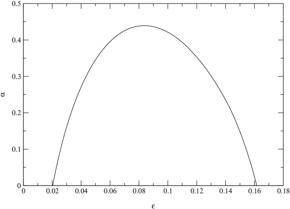
Figure 1: Exponent $\alpha(\epsilon)$ as a function of the energy density $\epsilon$. The ground state energy is defined by $\alpha(\epsilon_{0})=0$. We find $\epsilon_{0}=0.0202845$.

In Fig.1 we show the exponent $\alpha$ as a function of the energy density $\epsilon$. For the sake of clarity we present only the region of positive values of $\alpha$. The lowest value of $\epsilon$ at which the exponent $\alpha$ vanishes, denoted by $\epsilon_{0}$, gives a lower bound to the ground-state energy density of the spin model defined by the Hamiltonian (2) [30]. We find $\epsilon_{0}=0.0202845$ which, within the numerical precision, is exactly the value predicted by the first step of replica-symmetry breaking [4] as well as by Golay’s ergodicity hypothesis [15, 3]. This coincidence between the replica and the density of metastable states predictions for the ground-state energy occurs also in the random energy model [11, 16].

A similar study of the symmetrized version of the mean-field Hamiltonian (2), in which $J_{ij}^{k}=J_{ji}^{k}$, yields exactly the same expression for the exponent $\alpha$, see eq.(13), provided that the energy density $\epsilon$ is replaced by $\epsilon_{s}/2$. Hence the symmetrization procedure results in a trivial rescaling the energy densities of the local minima, without affecting their number.

3 Energy Barriers and Basin Sizes

The picture that comes out of the replica approach to disordered spin models is that the phase space $V$ composed of the $2^{N}$ spin configurations is broken into several valleys connected by saddle points [22]. The relative location and energetic properties of valleys and saddles are expected to determine e.g. the ease with which the ground state can be reached.

It will be convenient to introduce the notion of saddle-point energy $E[s,w]$ between two (not necessarily strict) minima $s$ and $w$. Denoting, for the sake of generality, the energy of state $x$ by $f(x)$, we can write

$$E[s,w]=\min\left\{\max\left[f(z)\big{|}z\in\mathbf{p}\right]\,\bigg{|}\,\mathbf{p}:\textrm{path from }s\textrm{ to }w\right\},$$ (14)

where a path $\mathbf{p}$ is a sequence of configurations connected by one-spin flips (or, more generally, by moves taken from any desired “move set”). The saddle-point energy $E[s,w]$ forms an ultrametric distance measure on the set of local minima, see e.g. [25, 31]. The barrier enclosing a local minimum is the height of the lowest saddle point that gives access to an energetically more favorable minimum. In symbols:

$$B(s)=\min\left\{E[s,w]-f(s)\big{|}w:f(w)<f(s)\right\}$$ (15)

If $B(s)=0$ then the local minimum $s$ is marginally stable. It is easy to check that eq.(15) is equivalent to the definition of the depth of local minimum in [18]. It agrees for metastable states with the more general definition of the depth of a “cycle” in the literature on inhomogeneous Markov chains [1, 6, 7].

The information contained in the energy barriers is conveniently summarized by two global parameters that e.g. determine the convergence behavior of Simulated Annealing and related algorithms. The depth of a landscape [17, 6, 18, 27] is defined as

$$\mathsf{D}=\max\left\{B(s)\big{|}s\textrm{ is not a global minimum }\right\}.$$ (16)

It can be shown that Simulated Annealing converges almost surely to a ground state if and only if the cooling schedule $T_{k}$ satisfies $\sum_{k\geq 0}\exp(-\mathsf{D}/T_{k})=\infty$ [17]. In order to make the depth comparable between different landscapes we shall consider below the dimensionless parameter $\mathsf{D}/\sigma$, where $\sigma^{2}$ is the variance of the energy across the landscape. A related quantity is the (dimensionless) difficulty [6, 7] of the landscape, defined by

$$\psi=\max\bigg{\{}\frac{B(s)}{f(s)-f(\min)}\bigg{|}s\textrm{ is not a global minimum}\bigg{\}}$$ (17)

where $f(\min)$ is the global energy minimum and the maximum is taken over non-global minima only. It is directly related to the optimal speed of convergence of Simulated Annealing.

Since a direct evaluation of eq.(14) would require the explicit constructions of all possible paths it does not provide a feasible algorithm for determining $E[s,w]$ even if $N$ is small enough to allow an exhaustive survey of the landscape. The values of $E[s,w]$ and $B(s)$ can, however, be retrieved from the barrier tree of the landscape. Barrier trees have been considered recently in the context of RNA folding [12] and under the name “disconnectivity graphs” in the protein folding literature [2, 14]. In this contribution we use a modified version of the program barriers, which was developed for the analysis of RNA folding landscapes in [12]. For the sake of completeness we briefly outline the definition of the barrier trees below.

Figure 2: Example of a barrier tree of a landscape. Data belong to a Gaussian REM with $N=7$. The leaves 1-12 denote the local minima. The global minimum 1 is marked with an asterisk. Saddle points are labelled with capital letters from A to G. The saddle points $\mathsf{B}$, $\mathsf{C}$, $\mathsf{D}$, $\mathsf{E}$ are “degenerate” indicating that the lowest energy paths leaving e.g. 4,5,8 run through a common exit point. (Note that all $2^{7}=128$ configurations have pairwise distinct energies, hence there are no two distinct saddle points with the same energy, which may exist e.g. in the LABSP.) The Barrier of $5$ is $B(5)=E(\mathsf{D})-E(5)$, along the lowest path from $5$ to $4$, while $B(4)=E(\mathsf{E})-E(4)$, along the lowest path from $4$ to $1^{*}$.

For simplicity let us assume that the energies of any two spin configurations are distinct, i.e., there is a unique ordering of the spin configurations by their energies. The construction of the barrier tree starts from an energy-sorted list of all configurations in the landscape. We will need two lists of valleys throughout the calculation: The global minimum $x[1]$ belongs to the first active valley $V_{1}$, while the list of inactive valleys is empty initially. Going through this list of all configurations in the order of increasing energy we have three possibilities for the spin configuration $x[k]$ at step $k$.

• $x[k]$ has neighbors in exactly one of the active valleys $V_{i}$. Then $x[k]$ belong to $V_{i}$.

• $x[k]$ has no neighbor in any of the (active or inactive) valleys that we have found so far. Then $x[k]$ is a local minimum and determines a new active valley $V_{l}$. In the barrier tree $x[k]$ becomes a leaf.

• $x[k]$ has a neighbor in more than one active valley, say $\{V_{i_{1}},V_{i_{2}},\dots,V_{i_{q}}\}$. Then it is a saddle point connecting these active valleys. In the barrier tree $x[k]$ becomes an internal node. In this case we add $x[k]$ to valley $V_{i_{1}}$ with the lowest energy. Then we copy the configurations of $V_{i_{2}},\dots,V_{i_{q}}$ to $V_{i_{1}}$. Finally, the status of $V_{i_{2}}$ through $V_{i_{q}}$ is changed from active to inactive. This reflects the fact that from the point of view of a configuration with an energy higher than the saddle point $x[k]$, $V_{i_{1}},\dots,V_{i_{q}}$ appear as a single valley that is subdivided only at lower energy. Consequently, after the highest saddle-point energy has been encountered, all valleys except for the globally optimal $V_{1}$ are in the inactive list.

The outcome of this procedure is a tree such as the one shown in Fig. 2. The leaves correspond to the valleys of the landscape, while the interior nodes denote the saddle points. The tree contains the information on all local minima and their connecting saddle points. Indeed, saddle-point energies, and energy barriers can be immediately read off the barrier trees.

    

    

Figure 3: Tree representation of typical landscapes with $N=16$. Upper left LABSP, upper right mean-field approximation, lower left integer 4-spin model, lower right Gaussian REM for $N=14$ since for $N=16$ the number of minima is too large to allow a meaningful drawing.

A precise definition of valleys and saddle points in a landscape requires that we take into account the degeneracies in the energy function, i.e., the existence of distinct spin configurations with identical energies, in particular, the presence of neutrality, where neighboring configurations have identical energies [26]. Degeneracies complicate the construction of the barrier tree, since the energy-sorting of the landscape is not unique any more. The simplest remedy is to use the same procedure as above starting from an arbitrary energy sorting. In this case the order of degenerate configurations in the list is arbitrary but fixed throughout the computation. Before proceeding to a configuration with strictly higher energy a simple clean-up step needs to be included in the tree-building algorithm: adjacent valleys with $E[s,w]=f(s)=f(w)$ are joined to a single valley. Note that the resulting barrier tree may still contain distinct valleys with the same energy, as the examples in Fig. 3 show. The leaves of the barrier trees are in general valleys which may contain more than one degenerate local minimum.

There is a clear visual difference between the barrier trees for LABSP and the mean-field approximation MF at the one hand, and the $\pm 1$ 4-spin Hamiltonian and the REM on the other hand. The main difference appears to be a much larger amount of degeneracy in LABSP/MF, in particular highly degenerate ground states. In fact, it can be shown that the pure Hamiltoninan (1) has many nontrivial symmetries, besides the trivial one where $x$ is replaced by $-x$, which are then responsible for the high degeneracy observed in the tree barrier [21]. Obviously, the disordered Hamiltonian (2) cannot have the same symmetries as the pure one, and so its high degeneracy stems simply from the extreme dilution of the couplings $J_{ij}^{k}$. All models, except REM, are symmetric under replacing $x$ by $-x$, hence all states appear in pairs. We note that the barrier tree of the $\pm 1$ 4-spin model is reminiscent of the “funnels” discussed e.g. in protein folding, with a large energy difference between the two global optima and almost all local “traps”. In contrast, the REM shows, as expected, no relationship between energy and nearness of local minimum to the global one.

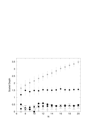
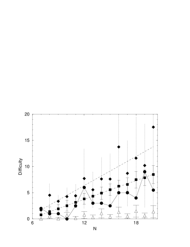
Figure 4: Depth and Difficulty. Symbols: $\bullet$ LABSP, $\blacksquare$ mean-field approximation, $\triangle$ $\pm 1$-version of the $2$-spin model, $\blacklozenge$ $\pm 1$-version of the $4$-spin model, $\star$ Gaussian REM. Data are averaged over 100 instances (50 instances for $N=20$); the error bars show the width of the distribution, not the standard error of the means.

During the construction of the barrier tree it is easy only to compute the lowest barrier $B^{\prime}(s)$ from $s$ to a local minimum that comes earlier in the list of configurations, instead of the lowest barrier $B(s)$ to a local minimum with strictly smaller energy. Clearly, $B^{\prime}(s)\leq B(s)$ since we take the minimum over a few more configurations than prescribed by eq.(15). In case of degenerate landscapes our version of the barriers program calculates $B^{\prime}(s)$ which depends on the ordering of the degenerate configurations. We obtain, however, $B(s)=B^{\prime}(s)$ for at least one of the valleys at each energy level. The fact that in eq.(16) we are required to maximize in particular over the barriers necessary to escape from any given energy level, however, implies that the values of depth and difficulty can be obtained directly from $B^{\prime}(s)$ instead of $B(s)$. We note at this point that a modified version $\mathsf{D}^{\prime}\geq\mathsf{D}$ of the depth in which the maximum over all non-global minima is replaced by the maximum over all minima except one global minimum $x^{*}$ can also be obtained by the simplified procedure above, since it can be shown that $\mathsf{D}^{\prime}$ is independent of the choice of $x^{*}$ [7]. The parameter $\mathsf{D}^{\prime}$ also appears in exact results on the convergence of Simulated Annealing.

Depth and Difficulty are shown in Figure 4 as a function of the number $N$ of spins. While there are (moderate) quantitative differences, there does not seem to be a qualitative difference between the LABSP, the mean-field approximation, and the discretized 2 and 4-spin models. Note that all landscapes with the exception of the Gaussian REM have constant scaled depth $\mathsf{D}/\sigma$, while $\mathsf{D}/\sigma$ increases linearly with the system size in the REM.

A linear regression of the difficulties yields the slopes $0.595\pm 6$, $0.926\pm 14$, and $0.07\pm 2$ for the mean-field Hamiltonian, the $\pm 1$-version of the $4$-spin model and the $\pm 1$ 2-spin model, respectively. As expected, the difficulty of the quadratic model is much smaller than the difficulty of the 4-spin model. For the sake of clarity, we have omitted the data about the mean difficulty of the REM since it is too large as compared to those shown in the figure. Moreover the width of its difficulty distribution is also so large that the mean value is not physically meaningful.

Figure 5: The logarithm of the size of the gradient-walk basin of attraction of the minima as function of their energies for $N=20$. The data for MF and the $\pm 1$ 4-spin model are superpositions of 10 instances, while for the REM we show only a single instance.

Additional information on the local minima can be traced during the construction of the barrier tree. We say that a configuration $x$ belongs to the basin of the local minimum $s$ if $s$ is the endpoint of the gradient walk (steepest descent) starting in $x$. (Recall that each step of a gradient walk goes to the lowest energy neighbor.) By determining the valley to which the lowest energy neighbor of $x[k]$ belongs we may for instance record the basin size of each local minimum. In a landscape without neutrality the gradient walk is uniquely determined by the initial condition, hence the basins form a partition of the set of configurations. We neglect the effects of neutrality in our numerical data by directing the gradient walk to the first possibility in the energy-sorted list of configurations.

Computationally we find, for all models but the REM, that there is an approximate linear relationship between the energy of a local minimum and the logarithm of the size of its gradient-walk basin of attraction, see Figure 5. The fact that the deepest valleys have the largest basins of attraction can be understood as a consequence of the correlation between neighboring spin configurations in all landscapes with the exception of the REM, for which all low-energy minima have essentially the same size of basin of attraction.

4 Discussion

The performance evaluation of local search heuristics, in particular Simulated Annealing, in typical instances of optimization problems is a relatively new subject, where the existing criteria for measuring the hardness or difficulty of a problem are still not widely known or accepted, as compared to e.g. the more traditional worst-case analysis. In fact, on the one hand, one expects that the average number of local minima may serve as a measure of the problem hardness, while, on the other hand, one must concede that only local minima separated by high energy barriers are potential traps for the search heuristic. In this paper we combine the concepts of depth and difficulty from the Simulated Annealing literature to the average density of states calculations from the statistical mechanics of disordered systems to obtain a reasonably complete statistical description of the energy landscapes of several classic disordered models. The motivation is to compare the statistical features of these landscapes with the properties of a rather puzzling deterministic problem — the low autocorrelated binary string problem (LABSP) — which has been identified as a particularly hard optimization problem for search heuristics such as Simulated Annealing.

Our results indicate that there is only a quantitative difference between the depths and difficulties, as defined in the Simulated Annealing literature, of all models investigated, with the exception of the random energy model (REM) for which the complete lack of correlations between the energies of neighboring configurations results in a genuine golf-course type landscape. Hence, we have found no evidences of a golf-course like structure in the LABSP landscape, which resembles much more a correlated spin-glass model than the REM. It must be emphasized that although the pure LABSP model (1) may have a glass phase characterized by uncorrelated equilibrium states (at least its mean-field version has such a phase [4]), the mere existence of this phase is no evidence of a golf-course like structure which, as mentioned above, requires vanishing correlations between the energy values of neighboring spin configurations.

Perhaps the “golf-course” conjecture [3, 21] stems simply from the fact that for large $N$ the LABSP is a much more difficult problem for Simulated Annealing than the familiar quadratic spin glass, as shown in Fig. 4. Interestingly, the pairwise comparison between the problems indicates that those problems with the larger number of local minima have also the larger difficulty, the only exception being LABSP and the 4-spin glass model. It should therefore be interesting to use these two problems as a test-bed for validating the hardness criteria proposed in the Simulated Annealing literature.

Finally, our analysis has shown that the disordered, mean-field Hamiltonian ${\mathcal{H}}_{d}$, eq.(2), describes surprisingly well the qualitative (e.g. the barrier trees) as well as the quantitative (e.g. number and typical energy of local minima) features of the pure model ${\mathcal{H}}$, eq.(1).

Acknowledgements

Special thanks to Christoph Flamm for the source code of his program barriers. The work of JFF was supported in part by Conselho Nacional de Desenvolvimento Científico e Tecnológico (CNPq). The work of PFS was supported in part by the Austrian Fonds zur Förderung der Wissenschaftlichen Forschung, Proj. No. 13093-GEN. FFF is supported by Fundação de Amparo à Pesquisa do Estado de São Paulo (FAPESP). We thank FAPESP for supporting PFS’s visit to São Carlos, where part of his work was done.

References

References

- [1] R. Azencott. Simulated Annealing. John Wiley & Sons, New York, 1992.
- [2] O. M. Becker and M. Karplus. The topology of multidimensional potential energy surfaces: Theory and application to peptide structure and kinetics. J. Chem. Phys., 106:1495–1517, 1997.
- [3] J. Bernasconi. Low autocorrelation binary sequences: statistical mechanics and configuration space analysis. J. Physique, 48:559–567, 1987.
- [4] J. P. Bouchaud and M. Mézard. Self-induced quenced disorder: A model for the glass transition. J. Physique I France, 4:1109–1114, 1994.
- [5] A. J. Bray and M. A. Moore. Metastable states in spin glasses with short-ranged interactions. J. Phys. C, 14:1313–1327, 1981.
- [6] O. Catoni. Rough large deviation estimates for simulated annealing: Application to exponential schedules. Ann. Probab., 20:1109–1146, 1992.
- [7] O. Catoni. Simulated annealing algorithms and Markov chains with rate transitions. In J. Azema, M. Emery, M. Ledoux, and M. Yor, editors, Seminaire de Probabilites XXXIII, volume 709 of Lecture Notes in Mathematics, pages 69–119. Springer, Berlin/Heidelberg, 1999.
- [8] M. Cieplak and T. R. Gawron. Metastable states in disordered ferromagnets. J. Phys. A: Math. Gen., 20:5657–5666, 1987.
- [9] V. M. de Oliveira and J. F. Fontanari. Replica analysis of the p-spin interactions Ising spin-glass model. J. Phys. A: Math. Gen., 32:2285–2296, 1999.
- [10] V. M. de Oliveira, J. F. Fontanari, and P. F. Stadler. Metastable states in high order short-range spin glasses. J. Phys. A: Math. Gen., 32:8793–8802, 1999.
- [11] B. Derrida. Random energy model: Limit of a family of disordered models. Phys. Rev. Lett., 45:79–82, 1980.
- [12] C. Flamm, W. Fontana, I. Hofacker, and P. Schuster. RNA folding kinetics at elementary step resolution. RNA, 6:325–338, 2000.
- [13] E. Gardner. Spin glasses with p-spin interactions. Nucl. Phys. B, 257:747–765, 1985.
- [14] P. Garstecki, T. X. Hoang, and M. Cieplak. Energy landscapes, supergraphs, and “folding funnels” in spin systems. Phys. Rev. E, 60:3219–3226, 1999.
- [15] M. J. E. Golay. Sieves for low-autocorrelation binary sequences. IEEE Trans. Inform. Th., IT-23:43–51, 1977.
- [16] D. J. Gross and M. Mézard. The simplest spin glass. Nucl. Phys. B, 240:431–452, 1984.
- [17] B. Hajek. Cooling schedules for optimal annealing. Math. Operations Res., 13:311–329, 1988.
- [18] W. Kern. On the depth of combinatorial optimization problems. Discr. Appl. Math., 43:115–129, 1993.
- [19] E. Marinari, G. Parisi, and F. Ritort. Replica field theory for deterministic models: I. Binary sequences with low autocorrelation. J. Phys. A: Math. Gen., 27:7615–7646, 1994.
- [20] E. Marinari, G. Parisi, and F. Ritort. Replica field theory for deterministic models: II. a non-random spin glass with glassy behaviour. J. Phys. A: Math. Gen., 27:7647–7668, 1994.
- [21] S. Mertens. Exhaustive search for low-autocorrelation binary sequences. J. Phys. A: Math. Gen., 29:L473–L481, 1996.
- [22] M. Mézard, G. Parisi, and M. A. Virasoro. Spin Glass Theory and Beyond. World Scientific, Singapore, 1987.
- [23] G. Migliorini and F. Ritort. Dynamical behaviour of low autocorrelation models. J. Phys. A: Math. Gen., 27:7669–7686, 1994.
- [24] B. Militzer, M. Zamparelli, and D. Beule. Evolutionary search for low autocorrelated binary sequences. IEEE Trans. Evol. Comp., 2:34–39, 1998.
- [25] R. Rammal, G. Toulouse, and M. A. Virasoro. Ultrametricity for physicists. Rev. Mod. Phys., 58:765–788, 1986.
- [26] C. M. Reidys and P. F. Stadler. Neutrality in fitness landscapes. Appl. Math. & Comput., 2000. in press, Santa Fe Institute preprint 98-10-089.
- [27] J. Ryan. The depth and width of local minima in discrete solution spaces. Discr. Appl. Math., 56:75–82, 1995.
- [28] D. Sherrington and S. Kirkpatrick. Solvable model of a spin-glass. Phys. Rev. Lett., 35:1792–1795, 1975.
- [29] P. F. Stadler and B. Krakhofer. Local minima of p-spin models. Rev. Mex. Fis., 42:355–363, 1996.
- [30] F. Tanaka and S. F. Edwards. Analytic theory of ground state properties of a spin glass: I. Ising spin glass. J. Phys. F, 10:2769–2778, 1980.
- [31] A. M. Vertechi and M. A. Virasoro. Energy barriers in SK spin glass models. J. Phys. France, 50:2325–2332, 1989.