Parallel Excluded Volume Tempering for Polymer Melts

Abstract

We have developed a technique to accelerate the acquisition of effectively uncorrelated configurations for off-lattice models of dense polymer melts which makes use of both parallel tempering and large scale Monte Carlo moves. The method is based upon simulating a set of systems in parallel, each of which has a slightly different repulsive core potential, such that a thermodynamic path from full excluded volume to an ideal gas of random walks is generated. While each system is run with standard stochastic dynamics, resulting in an NVT ensemble, we implement the parallel tempering through stochastic swaps between the configurations of adjacent potentials, and the large scale Monte Carlo moves through attempted pivot and translation moves which reach a realistic acceptance probability as the limit of the ideal gas of random walks is approached. Compared to pure stochastic dynamics, this results in an increased efficiency even for a system of chains as short as $N=60$ monomers, however at this chain length the large scale Monte Carlo moves were ineffective. For even longer chains the speedup becomes substantial, as observed from preliminary data for $N=200$. While the previously established end-bridging algorithm relaxes the end-to-end autocorrelation function more quickly, it does so at the price of an artificial polydispersity, which the current method does not exhibit. The end-to-end autocorrelation function is however no longer the slowest mode for the end-bridging algorithm so whether the algorithm is superior even for the case of polydispersity is unclear.
PACS: 05.10Ln,61.20.Ja,61.25.Hq,61.41.+e,83.10.Nn

I Introduction

Computer simulations of dense polymer systems which make use of off-lattice models have been successful in the determination of both static properties, such as phase equilibria [1, 2, 3, 4] or rubber elasticity [5], and dynamic properties, such as the details of single-chain and collective relaxation [6, 7, 8, 9]. For a melt of polymers of length $N$, the relaxation time $\tau$, the time taken for the polymer to assume a new configuration, scales as $\tau\propto N^{2}$ for small $N$ (Rouse dynamics), while for larger $N$ reptation behavior, $\tau\propto N^{3}$ [6, 10] sets in. If the computer simulation of a polymer melt is performed in such a way that the dynamic properties are realistically reproduced then this scaling will be directly related to the computational effort needed to effectively sample phase space and obtain meaningful results for the static properties [11]. As a result progress in the simulation of systems involving polymers with large $N$ has been severely hampered.

A modern trend in Monte Carlo simulations in statistical physics is to strictly distinguish between simulations which only aim to determine the static properties of a given system, and those which also set out to determine the dynamic behavior. In the latter case one has to follow the natural motion of the system confined to local dynamics constrained by topology and/or barriers. If one is however only interested in generating uncorrelated configurations as quickly as possible, one can use an artificial dynamics which is able to reach new effectively uncorrelated configurations much more quickly than the physical dynamics would allow.

The Rouse scaling law $\tau\propto N^{2}$ is a direct consequence of only allowing local motions to occur. It is independent of any constraint to motion and holds even for phantom chains with no interaction whatsoever except connectivity. Clearly, violating locality is an important step if one wishes to accelerate the acquisition of uncorrelated configurations. Particularly successful examples of schemes which achieve this include cluster algorithms [12] for critical phenomena, and the pivot algorithm [13, 14] for isolated polymer chains, which collectively rotates a large part of the chain at once, thus allowing one to study the static properties for $N=10^{5}$ and above [14].

In a dense polymer system, however, such an approach will clearly fail, since practically any attempted large scale move will be rejected due to overlap with other monomers. The effective constraints to motion which cause these techniques to fail are of physical importance — this is the mechanism which, for sufficiently long chains, gives rise to the onset of the considerably slower reptation dynamics. As a result previous attempts to speed up simulations of polymer melts by only lifting locality are unable to alleviate the problem. For example, the continuum configurational biased Monte Carlo method (CCB, [15]) and its variants [16] remove a chain (partly), and attempt to regrow it into the existing matrix. This can in principle be seen as a non-local approach like the pivot algorithm, however, in a simulation of a dense polymer melt the chain will grow preferentially back into the cavity from which it was previously removed. This effect becomes more pronounced with increasing chain length.

A simulation algorithm geared at only generating uncorrelated equilibrium configurations should thus not only find a way to violate locality but also the constraints resulting from the topology of the system and/or barriers. Fortunately, techniques have been developed to achieve this. The multicanonical ensemble and its variants (also called “umbrella sampling”, “entropic sampling” or “$1/k$ sampling”) [17, 18, 19, 20, 21, 22] try to identify barriers and then introduce a suitable bias in order to remove them (i. e. to allow the system to easily enter these unfavorable states). Simulated tempering (also called “expanded ensemble”) [23, 24] tries to systematically soften the constraints to motion by giving the system access to different parameter values where the barriers are weaker.

While previous implementations of simulated tempering have mostly limited themselves to using an intensive variable of the ensemble, such as temperature or chemical potential, as the control parameter, an admittedly less intuitively obvious choice can however be made. The control parameter can instead originate from a term within the Hamiltonian of the ensemble itself. For a model of a polymer melt the strength of the excluded volume interaction is a particularly useful parameter, since it directly generates the topological constraints which ultimately give rise to reptation-like slowing down. This idea has already successfully been applied to lattice polymers for measuring chemical potentials [25, 26] and within the framework of a multicanonical ensemble [27], while for continuum polymers it has so far only been used in an ad hoc fashion for equilibration purposes [6, 8].

The present investigation is a first attempt to combine the virtues of both non-local updates and constraint removal for continuum models of dense polymer melts. The former is done via pivot moves [13, 14], while the latter is done via parallel tempering in the strength of the excluded volume interaction. Parallel tempering, also called “multiple Markov chains” [28, 29] or “exchange Monte Carlo” [30], is very similar in spirit to simulated tempering [23, 24], but offers a number of both conceptual and technical advantages.

Both approaches are based on studying a whole family of Hamiltonians ${\cal H}_{i}$, $i=1,\ldots,n$, each of which defines a standard Boltzmann weight $\exp\left(-{\cal H}_{i}\right)$, where, for convenience, the temperature has been absorbed into the definition of the Hamiltonian. This family of Hamiltonians will form a sequence in the one dimensional space of the control parameter. Along this line, the Hamiltonians must be located close enough to each other, such that the distribution of equilibrium states resulting from the Boltzmann weight $\exp\left(-{\cal H}_{i}\right)$ has significant overlap with the distributions given by the Boltzmann weights $\exp\left(-{\cal H}_{i-1}\right)$ and $\exp\left(-{\cal H}_{i+1}\right)$. A typical configuration for Hamiltonian ${\cal H}_{i}$ should be within the thermal fluctuations for both Hamiltonians, ${\cal H}_{i-1}$ and ${\cal H}_{i+1}$. As system size increases the distributions become sharper and sharper. As a result more and more Hamiltonians will be required for this condition to still be satisfied. One would thus in principle like to study a system which is as small as possible.

If we denote the control parameter by $\phi$, the above condition can be expressed as follows: For the averages of a given extensive variable $A$ in two adjacent ensembles characterized by $\phi$ and $\phi+\Delta\phi$ the relation

$$\left|\left<A\right>_{\phi+\Delta\phi}-\left<A\right>_{\phi}\right|\approx\left|\frac{\partial\left<A\right>}{\partial\phi}\right|\left|\Delta\phi\right|\hbox{$<\mkern-19.0mu\lower 4.0pt\hbox{$\sim$}$}\left(\left<A^{2}\right>_{\phi}-\left<A\right>_{\phi}^{2}\right)^{1/2}$$ (1)

should hold. Since

$$\left(\left<A^{2}\right>_{\phi}-\left<A\right>_{\phi}^{2}\right)^{1/2}\propto V^{1/2}$$ (2)

for reasons of Gaussian statistics and $\partial A/\partial\phi\propto V$, one finds $\Delta\phi\propto V^{-1/2}$ or $n$, the number of Hamiltonians in the sequence, $\propto V^{1/2}$.

Given a family of Hamiltonians with the above condition satisfied, the tempering procedure consists of allowing a given system to make stochastic switches to neighboring Hamiltonians on the sequence in parameter space at fixed system configuration. Ideally, this results in a diffusion process with respect to the Hamiltonians. In particular, a configuration which was originally subject to a “hard” Hamiltonian (with constraints) can diffuse to a “soft” Hamiltonian (without), relax there quickly, and return to the original hard Hamiltonian. This should, hopefully, accelerate the rate at which the system traverses phase space.

For a dense three-dimensional melt of flexible polymers one expects the following scaling: The time to diffuse along the path of Hamiltonians and back is proportional to $n^{2}\propto V$. Assuming that the soft Hamiltonian does not provide any constraints, and that a suitable algorithm is able to generate there a completely new configuration in practically zero relaxation time, one finds altogether $\tau\propto V$. Furthermore, the smallest system one can study is given by equating the linear box size to the mean end-to-end distance $R\propto N^{1/2}$ (in a melt the conformations are random walks [10]). Thus $\tau\propto V\propto N^{3/2}$, which is somewhat better than plain Rouse relaxation, $\tau\propto N^{2}$, and considerably faster than reptation, $\tau\propto N^{3}$. Nevertheless, it should be noted that the well-known slithering-snake algorithm [14] scales as $\tau\propto N^{\approx 1}$, i. e. is expected to be asymptotically even better than our procedure. For very dense systems the prefactor in this law will however be large, due to small acceptance rates of the slithering-snake moves, such that one might need unrealistically long chains in order to actually observe the superiority. Where we expect the biggest payoff for our algorithm, however, is in systems where the (true physical) dynamics is governed by an activated process, such as star polymers [31], where

$$\tau\propto\exp\left({\rm const.}N\right),$$ (3)

and for which the slithering-snake algorithm is not applicable. Regardless of these considerations, our first tests have deliberately focused on melts of linear chains, since this is the system which is characterized best with respect to both statics and dynamics.

The difference between simulated tempering and parallel tempering originates in how this idea is put into practice. Standard simulated tempering [23, 24] considers only one system, whose configurations we denote by $\vec{x}$, and simply adds the parameter $\phi$ as an additional degree of freedom, which is treated via a standard Monte Carlo algorithm in that expanded state space. This procedure is governed by the Hamiltonian ${\cal H}(\phi,\vec{x})-\eta(\phi)$, where $\eta$ is a suitable pre-weighting factor, to be determined self-consistently in order to prevent the simulation from getting trapped in the softest Hamiltonian. The partition function of the resulting expanded ensemble is given by

$$Z=\sum_{i}\exp\left(\eta_{i}\right)\int d\vec{x}\exp\left(-{\cal H}_{i}\right)=\sum_{i}\exp\left(\eta_{i}-F_{i}\right),$$ (4)

where $F$ is the free energy (temperature is again absorbed in the definition). Since the arguments of the exponentials are extensive, the sum will always be strongly dominated by the largest term, unless all of them are practically identical. This means that unless $\eta_{i}\approx F_{i}$ $\forall$ $i$ the system will not be able to traverse the full extent of the available parameter space as one or more parameter values will become highly improbable.

In parallel tempering $n$ systems are run in parallel, each of which is assigned one of the Hamiltonians ${\cal H}_{i}$. Diffusion in Hamiltonian space is then facilitated by simple swaps of the configurations of adjacent Hamiltonians. Since each Hamiltonian will always be occupied, there is no problem of the simulation not visiting any particular “unfavorable” Hamiltonian, and thus it is no longer necessary to determine pre-weighting factors. Furthermore, the scaling considerations from above remain valid; the increased CPU effort by a factor of $n$ is rewarded by the fact that we now have $n$ random walkers available to produce data. The series of $n$ systems can be seen as one extended ensemble with the partition function

$$Z = \int d\vec{x}_{1}\ldots d\vec{x}_{n}\frac{1}{n!}\sum_{p}$$ (6)

$$\exp\left(-{\cal H}_{p(1)}(\vec{x}_{1})\right)\ldots\exp\left(-{\cal H}_{p(n)}(\vec{x}_{n})\right)$$

$$= \prod_{i}Z_{i},$$ (7)

where $p$ denotes the possible permutations of the index set $i=1,\ldots,n$, and we have made use of the arbitrariness in labeling. Thus the method just simulates $n$ statistically independent systems.

The detailed balance condition for the swap is derived in a straightforward manner: If we denote two systems in which we attempt to switch the Hamiltonians by $\vec{x}$ (governed initially by Hamiltonian ${\cal H}_{1}$) and $\vec{y}$ (governed initially by Hamiltonian ${\cal H}_{2}$), then the transition probabilities $w$ must satisfy

$$\frac{w\left(\left(\vec{x},\vec{y}\right)\to\left(\vec{y},\vec{x}\right)\right)}{w\left(\left(\vec{y},\vec{x}\right)\to\left(\vec{x},\vec{y}\right)\right)}=\frac{P_{eq}(\vec{y},\vec{x})}{P_{eq}(\vec{x},\vec{y})}$$ (8)

$$= \exp\left(-{\cal H}_{1}(\vec{y})-{\cal H}_{2}(\vec{x})+{\cal H}_{1}(\vec{x})+{\cal H}_{2}(\vec{y})\right)=:B$$ (9)

(the partition functions cancel out in the ratio of equilibrium distributions). Using the standard Metropolis rule, the attempted swap $(\vec{x},\vec{y})\to(\vec{y},\vec{x})$ is accepted with probability $\min(1,B)$.

Given the simplicity of the method, and its potential, one should expect that its popularity will increase substantially in the future. So far, its use has not been very widespread, partly due to the fact that access to massively parallel computing facilities (for which the approach is ideally suited) is still somewhat limited. Applications up to now have included spin glasses [30], liquid-vapor phase coexistence [32], and several studies on the theta collapse of single polymer chains, and related issues, where always the temperature was used as the control parameter [29, 33, 34, 35, 36, 37, 38]. The fact that the strength of the excluded volume interaction could be used as a parameter in parallel tempering is mentioned in Ref. [27]; however, no actual run data were presented.

The remainder of this paper is organized as follows: In Sec. II we describe the details of model and algorithm. Section II A defines the standard Kremer-Grest model of a polymer melt [6], and its simulation by means of stochastic Langevin dynamics. Section II B then describes the most important ingredients of our parallel tempering procedure, which is based upon altering the functional form of the repulsive core potential and replacing it by a non-divergent “soft-core” potential, until the limit of phantom chains is reached. This allows the chains to pass through each other, thus eliminating the slow reptation dynamics. When the repulsive core potential is soft enough we will be able to perform pivot and whole polymer translation moves in the melt for which $\tau\propto N^{\approx 0}$, as described in more detail in Sec. II C. We also compare with end-bridging [39, 40], a very fast Monte Carlo algorithm which however does not conserve the chain lengths, and whose basic features are outlined in Sec. II D. Section III reports our numerical results. Section III A describes how we found the parameters for our procedure, while important time correlation functions to measure the efficiency of our algorithm are defined and presented in Sec. III B, resulting in our conclusion (Sec. III C).

II Model and Algorithm

A Kremer-Grest Model and Langevin Dynamics

The Kremer-Grest model [6] is one of several off-lattice models for polymer melts which are commonly known as “bead-spring” models. All particles have purely repulsive Lennard-Jones cores of the form

$$U_{LJ}(r) = 4\epsilon\left[\left(\frac{\sigma}{r}\right)^{12}-\left(\frac{\sigma}{r}\right)^{6}+\frac{1}{4}\right]\hskip 28.90755ptr\leq 2^{1/6}\sigma,$$ (10)

$$U_{LJ}(r) = 0\hskip 133.69994ptr\geq 2^{1/6}\sigma,$$ (11)

where $\epsilon$ and $\sigma$, as well as the bead mass, are set to unity such that time is in Lennard-Jones units. The FENE attraction between the neighboring monomers on the chains is given by

$$U_{ch}(r)=-\frac{k}{2}R_{0}^{2}\ln\left(1-\frac{r^{2}}{R_{0}^{2}}\right),$$ (12)

where $R_{0}=1.5$ is the maximum extension of the nonlinear spring, and $k=30$ is the spring constant. The spring constant is set to be strong enough to prohibit two polymer chains from crossing each other. We consider a system of $M$ chains of length $N$ in a cubic box with periodic boundary conditions at constant volume with density $\rho=0.85$.

We have simulated an NVT ensemble of this system through the use of Langevin (stochastic) dynamics [6, 11], fixing the temperature at $k_{B}T=1.0$ where $k_{B}$ denotes Boltzmann’s constant. This involves the addition of a random force and a friction term, resulting in the following equations of motion in terms of particle positions $\vec{r}_{i}$ and momenta $\vec{p}_{i}$:

$$\dot{\vec{p}_{i}} = \vec{F}_{i}-\frac{\gamma}{m_{i}}\vec{p}_{i}+\vec{f}_{i},$$ (13)

$$\dot{\vec{r}_{i}} = \frac{\vec{p}_{i}}{m_{i}},$$ (14)

where $\vec{F}_{i}$ is the force due to the interactions with other monomers, $m_{i}$ the particle mass, $\gamma$ the friction constant, and $\vec{f}_{i}$ the stochastic force which satisfies the standard fluctuation-dissipation relation

$$\left<f_{i\alpha}(t)f_{j\beta}(t^{\prime})\right>=2\gamma k_{B}T\delta_{ij}\delta_{\alpha\beta}\delta(t-t^{\prime})$$ (15)

(i. e. uncorrelated with respect to both particle indices $i$ and Cartesian indices $\alpha$). These equations were solved using the standard velocity Verlet integrator [11, 41], with friction coefficient $\gamma=0.5$ and time step $\Delta t=0.0125$.

Both statics and dynamics of this model are known very well [6, 11]. In particular, its slow Rouse- or reptation-like dynamics serves as a reference for the speedup obtained from our new Monte Carlo procedure.

B Parallel Tempering

We have performed parallel tempering by connecting a series of systems to the Kremer-Grest potential using successively softer repulsive core potentials. The $n$ systems are simulated in parallel, and each system is on a separate processor of a massively parallel system (Cray T3E). Once an initial locally equilibrated configuration (in real and momentum space) is obtained for each of the systems, the potentials are allowed to switch between systems through Metropolis Monte Carlo steps, as described above. It should be noted that the kinetic energies cancel out in the Metropolis criterion. The swaps are implemented in a checkerboard fashion, where either the odd-even pairs or the even-odd pairs are tried. Between these swaps each system is run for a few stochastic dynamics steps; it is known that this procedure is quite efficient for equilibrating local degrees of freedom. For example, if we were to use eight processors we would first attempt to switch the systems $1-2$, $3-4$, $5-6$, and $7-8$, then run some stochastic dynamics, then attempt the switches $2-3$, $4-5$, and $6-7$, then run more stochastic dynamics before attempting the first set of switches again. Fig. 1 shows how this aspect of the algorithm is implemented. A reasonable duration for the Langevin runs between the swaps is obtained from studying the potential energy relaxation, as described later.

In order to achieve large acceptance rates for the swaps it is necessary to choose the form of the “softened core” potential such that the bond length $b$ and the chain stiffness $C_{\infty}$ are approximately maintained. The core repulsion of the neighbors and next-nearest neighbors on chains were thus kept intact, while all other repulsive Lennard-Jones potentials were replaced by the following “softened core” potential

$$U_{SC}(r) = A-Br^{2}\hskip 88.89178ptr\leq r_{t},$$ (16)

$$U_{SC}(r) = 4\epsilon\left[\left(\frac{\sigma}{r}\right)^{12}-\left(\frac{\sigma}{r}\right)^{6}+\frac{1}{4}\right]\hskip 14.45377ptr_{t}\leq r\leq 2^{1/6}\sigma,$$ (17)

$$U_{SC}(r) = 0\hskip 121.41307ptr\geq 2^{1/6}\sigma,$$ (18)

where $A$ and $B$ are fixed by the continuity of $U(r)$ and $\frac{dU}{dr}$ leaving $r_{t}$ as the only free parameter. For the Kremer-Grest potential $r_{t}=0$, and $r_{t}$ is successively larger for each softer potential until the final potential in the series has $r_{t}=r_{c}=2^{1/6}\sigma$, the cutoff radius, which is the case for phantom chains. A graph of such a family of potentials is shown in Fig. 2. We will refer to the ratio $r_{t}/r_{c}$ as the “soft-core parameter”. Observing Fig. 2 it becomes quite apparent why our tempering parameter is a superior choice to temperature for the Kremer-Grest model. Tempering in temperature would be the equivalent of altering the potential by a constant multiple. No matter how high a temperature reached the $r^{-12}$ divergence of the core would not be alleviated.

C Pivot and Translation Moves

When we reach systems with extremely soft repulsive core potentials then large scale motions within the systems will have observable transition probabilities. We must ensure that these large scale motions through phase space are such that only the parts of the potential which have been softened are affected. Thus the large scale motions should not affect any bond lengths or angles within the polymers. Large scale moves that fulfill this criterion are pivot and translation moves.

The pivot move involves rotating part of the polymer around the axis of a given bond. As shown in Fig. 3, all of the interactions which have not been softened are unchanged in this move. The translation move involves taking the entire polymer and shifting it a random distance in a random direction. It is in reaching systems where these kinds of moves are possible before returning to the Kremer-Grest Hamiltonian where we expect our algorithm to pay off. We have implemented the pivot and translation moves together in a single move where the whole chain is simultaneously translated and every bond is rotated, thus relaxing all the degrees of freedom of the chain with the exception of the bond lengths and angles which are relaxed by the Langevin dynamics. We attempt these moves also quite frequently, as discussed later in the paper.

D End-Bridging

In order to compare our algorithm with an established Monte Carlo method for equilibrating dense polymer systems, we have also implemented an end-bridging procedure combined with Langevin dynamics. End-bridging, developed by Theodorou et al. [39, 40] is currently the most efficient algorithm; however, it gains its speed only by giving up monodispersity. Instead a fixed number of monomers and a fixed number of chains is simulated, whose length however is allowed to fluctuate within predefined limits. In practice, these limits are defined by allowing all chain lengths between $N(1-f)$ and $N(1+f)$, where $f$ is typically of order $1/2$. The algorithm involves allowing bonds within polymers to break and reattach to the ends of different polymers. It was originally devised for atomistic simulations with fixed bond lengths and involved an intricate procedure. Implementing this algorithm on the Kremer-Grest model, however, is far simpler since our bond lengths are able to fluctuate. The end of a chain searches for a possible chain to bridge to. This search is performed by finding all the monomers within the cutoff radius that are not on the same chain as the chain end in question. One out of these is selected at random. If a possible end-bridge is found then the move is accepted according to a Metropolis function where the Boltzmann factor is multiplied with a weight factor. This weight factor is given by the number of monomers which the end could possibly bridge to divided by the number of monomers the newly created end could bridge back to. This is necessary to satisfy detailed balance, i. e. to correct for the different probabilities to select the original reaction and the back reaction. A diagram of how end-bridging works for the Kremer-Grest model is shown in Fig. 4. In our implementation we run the Langevin dynamics for $10$ LJ time units, followed by $n_{br}$ bridging attempts, where $n_{br}$ is $20$ times the number of chains.

III Results and Discussion

A Construction of Simulation Procedure

We first tested the algorithm with a system of 20 chains of length 60. The effect of softening the potential is clearly seen in the standard pair correlation function $g(r)$, which is the probability to find a particle pair with distance $r$, normalized by the ideal gas value. This function is shown in Fig. 5, excluding the nearest and next-nearest neighbors on the polymer chains where the core repulsions are maintained at full strength. Compared to the fully repulsive system, there is a considerable probability for very short distances as soon as $r_{t}/r_{c}\hbox{$>\mkern-19.0mu\lower 4.0pt\hbox{$\sim$}$}0.95$, reflecting the ability of chains to pass through each other. This removes the topological constraints for chains of arbitrary length. Thus even without pivot moves the dynamics would not be slower than Rouse relaxation.

Furthermore, we measured the single-chain static structure factor $S(q)=N^{-1}\left<\left|\sum_{i}\exp(i\vec{q}\cdot\vec{r}_{i})\right|^{2}\right>$ for both the Kremer-Grest model and the phantom chains as shown in Fig. 6. As expected, the Kremer-Grest model reproduces the random walk exponent $\nu=0.5$, observed from the decay $S(q)\propto q^{-2}$. The result for the phantom chains is very similar to the Kremer-Grest model, indicating that the overall structure of the chain does not change very much as we soften the repulsive core potentials. This in turn means that no major chain rearrangements are necessary along the thermodynamic path, such that the transitions should be quite easy.

Nevertheless, it turned out that for our number of monomers one needs of the order of $10^{2}$ (due to computer restrictions we used 128) systems in order to connect from the fully repulsive potential to the phantom chain limit, requiring that the swap acceptance rates are of order $1/2$. The soft-core parameters were adjusted by hand, in essence via a trial-and-error procedure. A graph of the resulting transition probabilities for each of the potentials for both 20 chains of length 60 and 1200 purely repulsive Lennard-Jones particles is shown in Fig. 7. One clearly sees that in the soft limit the polymer system has much smaller swap rates than the corresponding system of Lennard-Jones particles. A possible explanation for this is that the chain connectivity induces increased density fluctuations and thus an increased sensitivity to small changes in the interaction. We expect this effect to become more and more pronounced with increasing chain length. This is a severe problem for this algorithm for two reasons. The algorithm will be slowed by an extra factor above and beyond that determined in our initial scaling analysis with increasing chain length and any pre-determination of an appropriate set of $r_{t}$ values based on a simple model with transferability to more complicated systems is precluded. In any implementation of this algorithm to a new problem the set of $r_{t}$ values for the specific model will have to be determined. We have not devised a systematic method for selection of the soft-core parameters. This would be a future improvement of the algorithm.

From measuring the time autocorrelation function of the potential energy for the untempered system (i. e. without swaps between potentials), shown in Fig. 8, we have found that the correlations decay very quickly after only a few time steps of Langevin dynamics and then cross over to a much slower decay. Our interpretation of the very fast initial decay is that it is a direct consequence of the local bond oscillations, which happen on roughly this time scale. This is also in accord with the observation that it occurs independently of the degree of softening, see Fig. 8, since the potentials between bond neighbors remained unchanged for all potentials. Conversely, the long-time behavior is quite strongly affected by the softening, again in agreement with the expectation that the function should decay much faster for a softer system. Furthermore, the energy-energy autocorrelation function is independent of chain length, as expected.

These results suggest that it is most efficient to attempt the switches frequently, on the time scale of the bond oscillations. We thus constructed the following algorithm: On every system we perform the large scale chain reorientation attempt on enough chains so that attempts are made to move at least 5% of the monomers. This is followed by 4 Langevin dynamics steps, after which the Hamiltonian swaps (either even-odd or odd-even) are performed. Then the procedure is repeated. For reasons of simplicity, we have applied the identical moves to all systems. It should be stated, in the interest of future development of this method, that this condition is however not necessary. Any algorithm which leaves the Boltzmann distributions of the different systems invariant will be valid. For our algorithm, however, as currently implemented, not to attempt the large-scale moves on the hard systems would only generate idle CPU time since the processors all have to wait for the slowest system to finish before attempting the next swap. A further optimization could however involve eliminating the large-scale moves on the hard systems, and replacing them by more Langevin steps. By fine-tuning this one should be able to reduce synchronization overhead to a minimum. We also found that as the soft-core parameter approaches the phantom chain limit local bond oscillations can become unstable. This can be easily remedied by increasing the friction in the Langevin dynamics as the soft-core parameter increases.

B Correlation Functions

An appropriate way to benchmark the program is to determine the CPU time needed per chain relaxed. Since every system periodically passes through the Hamiltonian with the full Lennard-Jones repulsive hard core potential, each system can be seen as a Kremer-Grest model which is sampled every time this Hamiltonian happens to lie on it. Useful single-chain quantities to measure are the normalized end-to-end vector autocorrelation function, $\left<\vec{R}(t)\cdot\vec{R}(0)\right>$ with $\vec{R}=\vec{r}_{N}-\vec{r}_{1}$ and the autocorrelation function of the lowest five Rouse modes, $\left<\vec{X}_{p}(t)\cdot\vec{X}_{p}(0)\right>$ with $p=1,\ldots,5$ and [8]

$$\vec{X}_{p}=\sqrt{2}N^{-1/2}\sum_{i=1}^{N}\vec{r}_{i}\cos\left[\frac{p\pi}{N}\left(i-1/2\right)\right].$$ (19)

These quantities must be measured in such a way that only correlations between configurations where the Kremer-Grest Hamiltonian is present are counted. Thus we define the following procedure to measure autocorrelation functions:

$$C(t)=\frac{\sum_{t^{\prime}}u(t^{\prime}+t)u(t^{\prime})\delta(U(t^{\prime}+t),U_{0})\delta(U(t^{\prime}),U_{0})}{\sum_{t^{\prime}}\delta(U(t^{\prime}+t),U_{0})\delta(U(t^{\prime}),U_{0})},$$ (20)

where $u(t)$ is the quantity whose autocorrelation function is determined, $U_{0}$ is the Kremer-Grest potential, and $U(t)$ the potential at time $t$. The Kronecker $\delta(U(t),U_{0})$ vanishes unless the potential is $U_{0}$ where it is unity.

Fig. 9 displays the normalized end-to-end vector autocorrelation function for (i) end-bridging with different degrees of polydispersity $f=0.4\ldots 0.6$, (ii) our simulated tempering procedure, and (iii) standard Langevin (Rouse-like) dynamics. It is seen that the end-bridging procedure is by far the fastest; however, it should be kept in mind that the speed comes at the price of considerable polydispersity. Furthermore, the end-to-end vector does not describe the slowest relaxation in the system for this type of algorithm. Since for the end-bridging algorithm what constitutes a polymer chain becomes an ill defined quantity, what actually does become the slowest mode is unclear. The simulated tempering procedure turns out to be somewhat faster than plain Rouse relaxation, in particular in the long-time limit. In terms of integrated autocorrelation time the speedup amounts to roughly 10 % with the pivot moves present and 30% without. The reason why pivoting actually slows the simulation down is explained from Figs. 10 and 11, which show the normalized end-to-end vector autocorrelation function and the autocorrelation of the first Rouse mode (in terms of “physical” time, not CPU time). The simple parallel tempering already needs such a long time for traversing Hamiltonian space from the ideal gas to the full repulsive interaction that on this time scale the chains are already fully relaxed. After a “diffusive loop” through Hamiltonian space the configuration is thus already fully decorrelated, even without pivot moves. Therefore the pivot moves just generate additional CPU overhead and cause a slowdown.

In Fig. 12 the autocorrelation of the lowest five Rouse modes vs. $t\sin^{2}(p\pi/2N)$ is shown. If Rouse scaling holds, then all Rouse modes should collapse onto a single line. As is known from older simulations [6, 8], $N=60$ is already slightly in the crossover regime to reptation, where ultimately the lower modes are slowed down. Nevertheless, $N=60$ is still too short for this effect to be become visible, such that Rouse behavior for the case of pure Langevin dynamics can still be assumed. Our tempering procedure, on the other hand, produces a disproportionate acceleration of the lower modes. They first decay exponentially in accord with the pure Rouse dynamics of the hard system. At later times, however, one observes a steeper exponential decay, which is the effect of the decorrelating excursions to the softer systems.

We were also able to obtain results, shown in Fig. 13, for a system of 32 chains of length 200, using 256 Hamiltonians. Limitations in the CPU time available to us have prevented us from performing a comparison between simulations with and without pivot moves, and from measuring the correlation function until full decay. Nevertheless, our preliminary data clearly show a steep drop off in the correlation functions, which is much more pronounced than for the case of $N=60$. These data were obtained for the case with pivot moves; we believe that they actually did help to accelerate the equilibration of this system. The data for pure Langevin dynamics without tempering were taken from Ref. [42]. Extrapolating our data, we guess that the speedup is a factor of five or even larger.

C Conclusions

Our results indicate that parallel tempering combined with large-scale chain moves is, in principle, a viable route to speeding up simulations of dense polymer systems. However, for chains of moderate length ($N=60$) the effort seems hardly worthwhile, since the increase in efficiency compared to simple Langevin dynamics is not spectacular. Nevertheless, it is expected that the method will pay off for systems with either longer chains, as indicated from our preliminary results for chain length $200$, or more complicated molecular architecture. These issues will be the subject of future investigations. Current trends in the development of computational facilities indicate that over the next decade we will see an increase in the availability of massively parallel computers with more and more processors running at approximately the speed of today’s processors. With the advent of such facilities we expect the full potential of this algorithm to be realized.

FIG. 1.: Schematic representation of our parallelization scheme. The double arrows represent attempted switches and the thick line represents the path through the Hamiltonians followed by one of the systems.

FIG. 2.: A set of successively softer repulsive core potentials. In the simulation we connect the system with the purely repulsive Lennard-Jones potential, shown as the solid line, through a series of such softened core repulsion potentials to the limit of phantom chains ($U=0$).

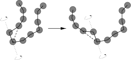
FIG. 3.: Schematic representation of our implementation of pivot moves: Neither the nearest neighbor nor the next-nearest neighbor distances on the polymer chain are affected. As a result none of the potential interactions which are kept at full strength are affected.

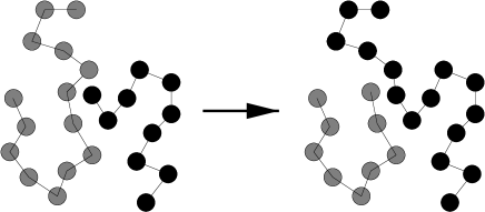
FIG. 4.: End-bridging move for the Kremer-Grest model. If the end-bridging move in question involves an energy change $\Delta E$ then the probability of the move is given by $P=\min(1,We^{-\Delta E})$ where $W$ is a weight factor given by the ratio between the number of possible monomers the initial end can bridge to and the number of monomers the newly created end could bridge back to.

FIG. 5.: Pair correlation function for several values of $r_{t}/r_{c}$. Note that starting at about $r_{t}/r_{c}=0.95$ the chains are effectively able to pass through each other.

FIG. 6.: Single-chain static structure factor for both the Kremer-Grest model and phantom chains. The similarity in the static structure factor indicates that the large scale structure of the chains is nearly invariant as the repulsive core potentials are softened. The straight line represents a slope of $-2$ corresponding to $\nu=0.5$.

FIG. 7.: Probability that a system would transfer to the next softer potential, as a function of its own potential index, which increases with softness.

FIG. 8.: Energy-energy correlation function as a function of time in Lennard-Jones time units. Note the very fast decay on short time scales followed by a much slower decay which is dependent on the soft-core parameter.

FIG. 9.: Normalized end-to-end vector autocorrelation function for standard Langevin dynamics, our parallel tempering procedure with and without pivot moves, and end-bridging simulations for various degrees of polydispersity.

FIG. 10.: Normalized end-to-end vector autocorrelation function for our parallel tempering algorithm with and without pivot moves.

FIG. 11.: Autocorrelation of the first Rouse mode for our parallel tempering algorithm with and without pivot moves.

FIG. 12.: Rouse mode analysis for the lowest five Rouse modes for our parallel tempering procedure and compared to the case of pure Langevin dynamics. Though we have shown only the result for the second Rouse mode, all Rouse modes fall onto the same line for pure Langevin dynamics.

FIG. 13.: Normalized autocorrelation of the first Rouse mode for our parallel tempering procedure for chain length $200$. We have compared our result to a fit to results previously obtained by M. Pütz[42].

REFERENCES

- [1] G. S. Grest, M.-D. Lacasse, K. Kremer, and A. Gupta, J. Chem. Phys. 105, 10583 (1996).
- [2] F. A. Escobedo and J. J. dePablo, J. Chem. Phys. 105, 4391 (1996).
- [3] F. A. Escobedo and J. J. dePablo, J. Chem. Phys. 106, 2911 (1997).
- [4] F. A. Escobedo and J. J. dePablo, J. Chem. Phys. 106, 9858 (1997).
- [5] R. Everaers, New J. Phys. 1, 12.1 (1999).
- [6] K. Kremer and G. S. Grest, J. Chem. Phys. 92, 5057 (1990).
- [7] M. Kröger, W. Loose, and S. Hess, J. Rheology 37, 1057 (1993).
- [8] A. Kopf, B. Dünweg, and W. Paul, J. Chem. Phys. 107, 6945 (1997).
- [9] W. Paul et al., Phys. Rev. Lett. 80, 2346 (1998).
- [10] M. Doi and S. F. Edwards, The Theory of Polymer Dynamics (Clarendon Press, Oxford, 1986).
- [11] B. Dünweg, G. S. Grest, and K. Kremer, in Numerical Methods for Polymeric Systems, edited by S. G. Whittington (Springer-Verlag, Heidelberg, 1998), p. 159.
- [12] R. H. Swendsen and J. S. Wang, Phys. Rev. Lett. 58, 86 (1987).
- [13] N. Madras and A. D. Sokal, J. Stat. Phys. 50, 109 (1988).
- [14] A. D. Sokal, in Monte Carlo and Molecular Dynamics Simulations in Polymer Science, edited by K. Binder (Oxford University Press, New York, 1995), p. 47.
- [15] D. Frenkel and G. Mooij, in Monte Carlo and Molecular Dynamics of Condensed Matter Systems, edited by K. Binder and G. Ciccotti (Societa Italiana di Fisica, Bologna, 1996), p. 163.
- [16] S. Consta, N. B. Wilding, D. Frenkel, and Z. Alexandrowicz, J. Chem. Phys. 110, 3220 (1999).
- [17] J. P. Valleau and G. M. Torrie, in Statistical Mechanics Part A: Equilibrium Techniques, edited by B. J. Berne (Plenum, New York / London, 1977).
- [18] G. M. Torrie and J. P. Valleau, J. Comp. Phys. 23, 187 (1977).
- [19] B. A. Berg and T. Neuhaus, Phys. Rev. Lett. 68, 9 (1992).
- [20] B. A. Berg, Int. J. Mod. Phys. C 3, 1083 (1992).
- [21] J. Lee, Phys. Rev. Lett. 71, 211 (1993).
- [22] B. Hesselbo and R. B. Stinchcombe, Phys. Rev. Lett. 74, 2151 (1995).
- [23] E. Marinari and G. Parisi, Europhys. Lett. 19, 451 (1992).
- [24] A. P. Lyubartsev, A. A. Martinovski, S. V. Shevkunov, and P. N. Vorontsov-Velyaminov, J. Chem. Phys. 96, 1776 (1992).
- [25] M. Müller and W. Paul, J. Chem. Phys. 100, 719 (1993).
- [26] N. B. Wilding and M. Müller, J. Chem. Phys. 101, 4324 (1994).
- [27] Y. Iba, G. Chikenji, and M. Kikuchi, J. Phys. Soc. Japan 67, 3327 (1998).
- [28] C. J. Geyer, Computing Science and Statistics: Proceedings of the 23rd Symposium of the Interface 156, 1991 (1991).
- [29] E. Orlandini, in Numerical Methods for Polymeric Systems, edited by S. G. Whittington (Springer-Verlag, Heidelberg, 1998), p. 33.
- [30] K. Hukushima, H. Takayama, and K. Nemoto, J. Phys. Soc. Japan 65, 1604 (1996).
- [31] T. C. B. McLeish and S. T. Milner, Adv. Polym. Sci. 143, 195 (1999).
- [32] Q. L. Yan and J. J. dePablo, J. Chem. Phys. 111, 9509 (1999).
- [33] M. C. Tesi, E. J. J. van Rensburg, E. Orlandini, and S. G. Whittington, J. Stat. Phys. 82, 155 (1996).
- [34] P. P. Nidras and R. Brak, J. Phys. A 30, 1457 (1997).
- [35] U. H. E. Hansmann, Chem. Phys. Lett. 281, 140 (1997).
- [36] E. Orlandini and T. Garel, Int. J. Mod. Phys. C 9, 1459 (1998).
- [37] E. J. J. van Rensburg, E. Orlandini, and M. C. Tesi, J. Phys. A 32, 1567 (1999).
- [38] A. Irbäck and E. Sandelin, J. Chem. Phys. 110, 12256 (1999).
- [39] P. V. K. Pant and D. N. Theodorou, Macromolecules 28, 7224 (1995).
- [40] V. G. Mavrantzas, T. D. Boone, E. Zervopoulou, and D. N. Theodorou, Macromolecules 32, 5072 (1999).
- [41] M. P. Allen and D. J. Tildesley, Computer Simulations of Liquids (Clarendon Press, Oxford, 1989).
- [42] M. Pütz, PhD thesis, University of Mainz (1999).