The Effect of Interaction on Shot Noise in The Quantum Limit

We calculate the current and the current noise in a diffusive micro-bridge in the presence of electron-electron interactions. Out of equilibrium the fluctuation-dissipation theorem (FDT) does not apply, hence these two quantities are not simply related to each other. For a two-dimensional electron gas (2DEG) we obtain logarithmic singularities in the low frequency limit. PACS Nos. 71.10.Ay, 71.23.An, 73.50.Td

1 Introduction

The physics of non-equilibrium mesoscopic systems has been the subject of extensive theoretical and experimental research for more than a decade $\!{}^{{\bf?},{\bf?},{\bf?}}$. The first step $\!{}^{{\bf?},{\bf?},{\bf?},{\bf?}}$ was the understanding that Fermi statistics has a dramatic effect on the noise in the quantum limit. Employing various methods ( e.g. semiclassical approximations $\!{}^{{\bf?}}$ the Landauer scattering states approach $\!{}^{{\bf?},{\bf?},{\bf?}}$ and diagrammatic Keldysh techniques $\!{}^{{\bf?}}$) it has been recognized that the zero frequency $\!{}^{{\bf?}}$ zero temperature noise vanishes in the limit of perfect transparency, while the conductance remains finite. For a multichannel geometry one obtains

$$S(0)=\frac{e^{2}}{\pi\hbar}\sum_{n}T_{n}(1-T_{n})eV\,\,,$$ (1)

where $\{T_{n}\}$ are the channel transparencies and $V$ is the voltage drop across the junction under consideration. This result may be used when discussing disordered conductors. Upon averaging over an ensemble of coherent diffusive systems (the size of which is smaller than any of the inelastic, dephasing and localization lengths), one obtains a universal $1/3$ reduction from the traditional expression for shot-noise $\!{}^{{\bf?}}$, $S=e<I>$ ( the expectation value with respect to the effective action, denoted by $<>$ , includes configuration averaging).

While the physics of non-interacting electrons ( especially when disorder averaging is involved) turns out to be quite universal, this is not the case when electron-electron interactions are present. Nevertheless, when the dynamics of the electrons is classical, rendering quantum mechanical interference effects negligible, one may resort to the physically appealing kinetic equation technique, or more specifically, employ the Kogan-Shulman $\!{}^{{\bf?}}$ approach. Under such conditions it is possible to define an effective single-particle distribution function which fluctuates in time and space. The characteristics of this distribution function , which affect the noise, depend on non-universal factors such as the external screening $\!{}^{{\bf?},{\bf?}}$, the geometrical details of the contacts $\!{}^{{\bf?}}$ and the various inelastic processes rates $\!{}^{{\bf?},{\bf?}}$ . One may then consider two limiting cases, namely the short and the long energy relaxation length. Correspondingly, and depending on the frequency range , one may obtain different suppression factors ( see e.g.$\!{}^{{\bf?},{\bf?}}$), or even a noise spectrum which depends on the spatial coordinate $\!{}^{{\bf?}}$. The dependence of the shot noise on both Fermi statistics and on the value of the discrete elementary charge has become manifest through experiments on fractional quantum Hall systems, where electron-electron interaction redefine the quasi-particle charge $\!{}^{{\bf?}}$.

Apart from the later effect, electron-electron interactions may introduce further non-trivial signatures. For interacting systems at equilibrium this has been studied by Altshuler and Aronov $\!{}^{{\bf?}}$, who found small albeit singular ( in the temperature) corrections to the linear conductivity ( hence, by FDT, to the equilibrium noise). These corrections to the noise are the result of an interplay between disorder and interaction, and depend on the coherence of the electrons. One might expect an analogous type of physics out of equilibrium. Pursuing the study of the effect of interactions beyond the scope of the kinetic equation and well into the quantum regime is the main focus of the present work.

2 Results

We consider here a high mobility disordered metallic bridge, whose Ohmic conductance is $G_{Ohm}$. This bridge is connected to two ideal leads , each merging adiabatically onto a respective reservoir. The reservoirs are assumed to be at equilibrium with chemical potentials differing by $eV$. The linear dimensions of the bridge are all larger than the elastic mean free path , $l$, yet much shorter than the inelastic length, $l_{in}$. As the problem is technically challenging, we resort to a model calculation ,taking the interaction to be short-ranged. Considering a low electron-electron collision rate, one may assume the temperature $T$ to be constant throughout the system $\!{}^{{\bf?}}$. It is now convenient to define $\zeta=\mbox{max}\{eV,T\}$; $g_{\Box}$ will denote the dimensionless conductance per square, $\hbar\nu D$, where $\nu$ is the single electron density-of-states and $D$ is the diffusivity. Our main result concerns the zero frequency noise which is written as

$$\mbox{S}=\mbox{S}_{0}+\delta\mbox{S}\,\,,$$ (2)

where the interaction corrections to the zero frequency noise are given by

$$\delta\mbox{S}\!=\!\frac{G_{Ohm}}{6\pi^{2}g}\bigg{[}2T\ln\left(\!\frac{\zeta\tau}{\hbar}\!\right)\!+\!eV\!\coth\left(\!\frac{eV}{2T}\!\right)\!\!\bigg{(}\!\ln\left(\!\frac{\zeta\tau}{\hbar}\!\right)\!+\!\ln\left(\!\frac{T\tau}{\hbar}\!\right)\!\!\bigg{)}\!\bigg{]}.$$ (3)

This result should be compared with the corresponding correction to the conductance. We have obtained

$$\delta G_{Ohm}=\frac{G_{Ohm}}{2\pi^{2}g}\ln\left(\frac{\zeta\tau}{\hbar}\right)\,\,.$$ (4)

At equilibrium , as long as FDT is applicable, the interaction correction to the current noise may be cast as a correction to the Ohmic part of the conductance $\!{}^{{\bf?}}$ . Our results , Eqs.(3) and (4), demonstrate that out of equilibrium this is not any more the case: while corrections to the conductance are determined by the larger of the temperature and the applied voltage, the most singular correction to the noise involves a temperature-dominated logarithmic singularity.

3 The Approach

We now present a brief description of our derivation. Full account of the analysis is presented elsewhre$\!{}^{{\bf?}}$ We took notice of the work of Kamenev and Andreev $\!{}^{{\bf?}}$ , who had addressed the physics of disordered interacting electron gas by deriving a sigma-model description $\!{}^{{\bf?}}$ defined on a Keldysh contour ( see also Ref. $\!{}^{{\bf?}}$). In their work $\!{}^{{\bf?}}$ the interaction has been accounted for by expanding around an (approximate) interaction-dominated saddle point , obtained through gauge transformation. Here we pursue the Kamenev-Andreev approach further, to include non-equilibrium effects $\!{}^{{\bf?}}$.

Our starting point is the Lagrangian density

$$\hat{{\cal L}}=\overline{\Psi}[\hat{G}_{0}^{-1}-U_{dis}]\Psi-\overline{\Psi}\overline{\Psi}\hat{\mbox{V}}\Psi\Psi\,\,.$$ (5)

Here $\hat{V}$ represents the electron-electron interaction ; the Schrödinger operator of an electron of mass $m$ in the presence of a vector potential $a$ is given by

$$\hat{G}^{-1}_{0}=i\hbar\frac{\partial}{\partial t}+\frac{\hbar^{2}}{2m}\left(\nabla-a\right)^{2}+\mu\,\,.$$ (6)

All energies are measured from the chemical potential $\mu$. The action now contains an integral over space and an integral in time over the Keldysh contour . Such a representation is particularly convenient for averaging over disorder, as the generating functional $Z[a]$ is identically equal to $1$ when the external sources on the forward and backward paths are equal.

Next , one averages over the $\delta$-correlated disorder. We then perform a Hubbard-Stratonovich transformation, introducing the bosonic fields $Q$ and $\Phi$ which decouple the non-local-in-time term (generated by disorder averaging) and the non-local-in-space term ( produced by the Coulomb interaction ) respectively. In terms of the bosonic matrix field $Q$ and $\Phi$ the action now reads

$$iS[\hat{Q},\hat{\Phi}]=i\mbox{Tr}\{\Phi^{T}\mbox{V}^{-1}\gamma_{2}\Phi\}\!-\frac{\pi\nu}{4\tau}\mbox{Tr}\{\hat{Q}^{2}\}\!+$$

$$\mbox{Tr}\ln\Big{[}\hat{G}_{0}^{-1}\!+\!\frac{i\hat{Q}\sigma_{3}}{2\tau}\!+\!\hat{\phi}_{\alpha}\hat{\gamma}^{\alpha}\Big{]}.$$ (7)

Unlike the original treatment of Ref.$\!{}^{{\bf?}}$, we presently try to avoid the overwhelming task of finding an interaction-gauged saddle-point solution out of equilibrium . Instead, we consider here short-ranged interaction which , we believe, captures the essentials of the problem at hand:

$$\hat{\mbox{V}}(x-x^{\prime})=\Gamma\delta(x-x^{\prime})\,.$$ (8)

Hereafter $\Gamma$ is assumed to be small $(\Gamma\nu\ll 1)$. For weak disorder $(\epsilon_{F}\tau\gg 1$ ,$\tau$ being the elastic mean free time) it is possible to separate the slow and fast degrees of freedom . Expanding around the noninteracting saddle point yields the following effective action

$$iS=\!i\Gamma^{-1}\mbox{Tr}\{\Phi^{T}\gamma_{2}\Phi\}\!-\!\frac{\pi\nu}{4}\mbox{Tr}\{D(\nabla\!Q)^{2}\!\!-\!4i\!(\phi_{\alpha}\gamma^{\alpha}\!+\!\hat{\epsilon})Q\}\,\,,$$ (9)

with the usual non-linear constraint $Q^{2}=1$. Here $\Phi^{T}=(\phi_{1},\phi_{2})$ and

$$\gamma_{1}=\left(\matrix{1&0\cr 0&1\cr}\right),\;\gamma_{2}=\left(\matrix{0&1\cr 1&0\cr}\right).$$ (10)

Within this model one may calculate the correlation function of the fluctuations of the electric potential

$$\langle\phi_{i}(r,\omega)\phi_{j}(r^{\prime},-\omega)\rangle\!=\!-i\Gamma\delta(r-r^{\prime})\gamma_{2}^{i,j}.$$ (11)

Let us first consider the non-interacting scenario , stressing a few points that were implicit in previous works $\!{}^{{\bf?},{\bf?}}$. The gapless fluctuations of $Q$ around the saddle point are conveniently parameterized as

$$Q=\Lambda\exp\left(W\right)\,\,,$$

$$\Lambda W+W\Lambda=0\,\,.$$ (12)

To satisfy the non-linear constraint on $Q$ and , at the same time , conform to Eq. (3), one may use the representation

$$W_{x,\epsilon,\epsilon^{\prime}}=\left(\matrix{F_{x,\epsilon}\bar{w}_{x,\epsilon,\epsilon^{\prime}}&-w_{x,\epsilon,\epsilon^{\prime}}+F_{x,\epsilon}\bar{w}_{x,\epsilon,\epsilon^{\prime}}F_{x,\epsilon^{\prime}}\cr-\bar{w}_{x,\epsilon,\epsilon^{\prime}}&-\bar{w}_{x,\epsilon,\epsilon^{\prime}}F_{x,\epsilon^{\prime}}\cr}\right)\,\,,$$ (13)

where the fields $\omega,\bar{\omega}$ are unconstrained. Expanding the action to second order in the soft modes yields for the free part of the action

$$iS[W]=iS^{0}[W]+iS^{1}[W]+iS^{2}[W]\,\,.$$ (14)

The zeroth order term vanishes at the saddle point. The linear part in $W$ should vanish as well, yielding an equation for $F$ which, together with the appropriate boundary conditions, determines $F$ uniquely The quadratic part of the action is equal to

$$iS^{2}[W]=\frac{\pi\nu}{2}\bigg{[}\bar{w}_{x,\epsilon,\epsilon^{\prime}}[-D\nabla^{2}+i(\epsilon-\epsilon^{\prime})]w_{x,\epsilon^{\prime},\epsilon}-$$

$$D\nabla F_{x,\epsilon}\bar{w}_{x,\epsilon,\epsilon^{\prime}}\nabla F_{x,\epsilon^{\prime}}\bar{w}_{x,\epsilon^{\prime},\epsilon}\bigg{]}\,\,.$$ (15)

The last term in (3) is responsible for equilibration along the longitudinal coordinate; it is absent at equilibrium.

Turning our attention now to the diffusive constriction geometry, we specifically consider the slow energy relaxation time limit. The distribution function is then readily calculated $\!{}^{{\bf?},{\bf?}}$. One may next evaluate various correlation functions for this system out of equilibrium. For our unconstrained Gaussian action, Eq. (3), they can be written in terms of the diffusion propogator $\!{}^{{\bf?}}$

$$\langle w(x,\epsilon_{1},\epsilon_{2})\bar{w}(x^{\prime},\epsilon_{3},\epsilon_{4})\rangle=2\delta_{\epsilon_{1},\epsilon_{4}}\delta_{\epsilon_{2},\epsilon_{3}}\mbox{D}(x,x^{\prime},\epsilon_{1}-\epsilon_{2})$$

$$\langle w(x,\epsilon_{1},\epsilon_{2})w(x^{\prime},\epsilon_{3},\epsilon_{3})\rangle=-\delta_{\epsilon_{1},\epsilon_{4}}\delta_{\epsilon_{2},\epsilon_{3}}2\pi\nu D$$

$$\mbox{D}_{\epsilon_{1}-\epsilon_{2},x,x_{1}}\nabla F_{\epsilon_{2},x_{1}}\otimes\nabla F_{\epsilon_{1},x_{1}}\mbox{D}_{\epsilon_{2}-\epsilon_{1},x_{1},x^{\prime}}\,\,.$$ (16)

Employing the above building blocks we may calculate the symmetrized current-current correlation function

$$\mbox{S}(t,x,t^{\prime},x^{\prime})=\frac{1}{2}\big{[}\langle\langle\hat{I}(t,x)\hat{I}(t^{\prime},x^{\prime})+\hat{I}(t^{\prime},x^{\prime})\hat{I}(t,x)\rangle\rangle\big{]}\,\,.$$ (17)

Under stationary conditions it is a function of the difference of its arguments. Relying on the identity $Z[a_{+},a_{-}=0]=1$ ( where the indices refer to the symmetric (“classical”) and the antisymmetric (“quantal”) combinations over the Keldysh branches) , we express S as

$$\mbox{S}(x,t;x^{\prime},t^{\prime})=-\frac{e^{2}}{4}\frac{\delta^{2}Z[a]}{\delta a_{2}(x,t)\delta a_{2}(x^{\prime},t^{\prime})}\,\,.$$ (18)

After functional differentiation one obtains the following equation

$$\mbox{S}_{x,t;x^{\prime},t^{\prime}}\!=\!\frac{e^{2}\pi\nu\!D}{4}\bigg{<}\!\mbox{I}^{D}_{x,t,t^{\prime}}\!\delta_{x,x^{\prime}}\!-\!\frac{\pi\nu\!D}{2}\mbox{M}_{x,t}\!\mbox{M}_{x^{\prime},t^{\prime}}\!\bigg{>}\!-\!\langle\mbox{I}\rangle^{2},$$ (19)

where we have introduced the notation

$$\mbox{I}^{D}_{x,t}=\mbox{Tr}\!\bigg{\{}\!Q_{x,t,t^{\prime}}\gamma_{2}Q_{x^{\prime},t^{\prime},t}\gamma_{2}\!-\!Q_{x,t,t^{\prime}}Q_{x^{\prime},t^{\prime},t}\bigg{\}}\delta_{x,x^{\prime}}$$

$$\mbox{M}_{x,t}=\mbox{Tr}\bigg{\{}\big{(}Q_{x,t,t_{1}}\nabla Q_{x,t_{1},t}-(\nabla Q_{x,t,t_{1}})Q_{x,t_{1},t}\big{)}\gamma_{2}\bigg{\}}\,\,.$$ (20)

Expanding Eq. (19) to first order in $1/g$ and to zeroth order in $\Gamma$ , we recover the results of the direct diagrammatic analysis of this problem $\!{}^{{\bf?}}$. The extra power of $g$ in the second term ( a non-local part ) cancels with $\langle\,\mbox{I}\,\rangle^{2}$. At high frequencies, dynamical fluctuations of the local density are feasible, leading to the dependence of the noise on the the spatial coordinates; this is not anymore the case at low frequencies, $\omega\ll E_{Th}$ , which is a direct consequence of particle conservation. In this limit S is given as a sum of three equilibrium spectral functions $\!{}^{{\bf?}}$

$$\mbox{S}_{0}(\omega)=\frac{1}{6}[4\mbox{S}^{eq}(\omega)+\mbox{S}^{eq}(\omega+eV)+\mbox{S}^{eq}(\omega-eV)]\,\,,$$ (21)

as has been found earlier $\!{}^{{\bf?}}$.

4 The Effect Of e-e Interaction

So far we have considered the leading part of the current noise. Now on we discuss corrections due to e-e interactions. We note that under the conditions specified above, the non-equilibrium quasi-particle distribution function is essentially of a (temperature and interaction smeared) double-step form. We first evaluate the interaction correction to the stationary value of electron current, $\delta\mbox{I}^{ee}$. Employing the relation

$$I=\frac{-e}{2i}\frac{\delta Z[a]}{\delta a_{2}}\,\,,$$ (22)

and using the action (Eq. 9), we obtain

$$\delta\mbox{I}^{ee}=\frac{e\pi\nu D(i\pi\nu)^{2}}{4}\langle\mbox{M}\,\mbox{Tr}\{\phi_{\alpha}\gamma^{\alpha}Q\}\mbox{Tr}\{\phi_{\beta}\gamma^{\beta}Q\}\rangle_{0}\,\,.$$ (23)

Employing the rules of Eq.3 , this leads to

$$\delta\mbox{I}^{ee}=\langle\mbox{I}\rangle\frac{\Gamma\nu}{2(2\pi)^{2}g}\ln\left(\frac{\zeta\tau}{\hbar}\right)\,\,.$$ (24)

Let us turn now to the calculation of the interaction correction to the current noise. To this end one evaluates Eq. (19), employing the interaction dependent action, Eq. (21) . In first order in the interaction we obtain

$$\delta\mbox{S}^{ee}(0)=\frac{e^{2}\pi\nu D}{4}\bigg{<}[I^{D}_{x,t,t^{\prime}}\delta_{x,x^{\prime}}\!-\!\frac{\pi\nu D}{2}M_{x,t}M_{x^{\prime},t^{\prime}}]$$

$$\mbox{Tr}\{\phi_{\alpha}\gamma^{\alpha}Q\}\mbox{Tr}\{\phi_{\beta}\gamma^{\beta}Q\}\bigg{>}\,\,.$$ (25)

To proceed , we first carry out the averaging over the fields $\phi$ in Eq. (4) employing Eq. (11) . This leads to a $\Gamma$ dependent expression written solely in terms of the matrices $Q$. We then expand in the fields $\omega,\bar{\omega}$ and perform contractions according to the rules of Eq.(3). For frequencies smaller than the Thouless frequency , the current-current correlation function does not depend on the choice of the cross-section : integration over the spatial coordinates will lead to the suppression of space-derivative terms. We finally obtain

$$\delta\!S^{ee}\!\!=\!\!\frac{G\!\Gamma\nu}{12\!\pi^{2}g}\!\!\bigg{[}\!2T\!\ln\left(\!\frac{\zeta\tau}{\hbar}\!\right)\!\!+\!eV\!\!\coth\left(\!\frac{eV}{2\!T}\!\right)\!\!\bigg{(}\!\!\ln\left(\!\frac{\zeta\tau}{\hbar}\!\!\right)\!+\!\ln\left(\!\!\frac{T\tau}{\hbar}\!\!\right)\!\!\bigg{)}\!\bigg{]}.$$ (26)

The derivation of Eqs. (24) and (26) involves some controlled approximations. The use of a short range interaction (assumed to be small, $\Gamma\nu\ll 1$) renders them model dependent.

To establish a relation with the “real” screened Coulomb interaction, we further propose the following heuristic picture: we argue that the correct prefactor in the expression for $\delta\mbox{I}^{ee}$ should not depend strongly on either the temperature or the voltage ; hence it can be restored based on equilibrium calculations $\!{}^{{\bf?}}$ ,

$$\delta\mbox{I}^{ee}=\langle\mbox{I}\rangle\frac{1}{2\pi^{2}g}\ln\left(\frac{\zeta\tau}{\hbar}\right)\,\,.$$ (27)

Comparing Eqs.(24) and (27) we are able to express $\Gamma$ in terms of the model-independent parameters of the problem , which leads to Eq.(4). This mapping will be employed for the expression for the noise as well, leading to Eq. 3. Hereafter we have assumed $\zeta\gg E_{Th}$, which is readily satisfied for macroscopic samples. We note that both the voltage and the temperature may serve as cut-offs for the logarithmic singularity. For $T\gg eV$ the singularity is governed by $T$, resulting in the Altshuler-Aronov correction to the conductance.

Considering the asymptotic high temperature behavior of Eq.(3), one notes that the equilibrium part is dominant. By the FDT Eq. (3) is related to the Altshuler-Aronov correction to the conductance $\!{}^{{\bf?}}$ , which is obtained from Eq. (4) by substituting $\zeta=T$:

$$\delta\mbox{S}=\frac{G_{Ohm}}{\pi^{2}g}T\ln\left(\frac{T\tau}{\hbar}\right),$$ (28)

or, alternatively, it is related to the correction to the mean current, Eq.(27).

In the large voltage limit, current fluctuations are dominated by the bias dependent shot noise. Note, though, that the interaction corrections to it are still determined by the temperature,

$$\delta\mbox{S}=\frac{G_{Ohm}}{6\pi^{2}g}e|V|\ln\left(\frac{T\tau}{\hbar}\right)\,\,.$$ (29)

The FDT breaks down manifestly , and the results for the current (Eq. 27) and for the current noise (Eq. 29) are no longer related to each other in a simple way. Moreover, the interaction correction to the current noise is larger (for large bias ) than the corresponding correction to the mean current. On a qualitative level we note that within a classical picture,the electron-electron interaction may indeed lead to strong suppression of current fluctuations without affecting the mean current much, in agreement with our quantitative analysis. In other words, the relation between the mean current and the noise , $S\sim eI$, which is valid for Poisson-like processes, is no longer applicable. While we have presented here specific expressions for the interaction corrections in two dimensions, we do expect effects of similar nature to take place at other dimensions as well.

   
   

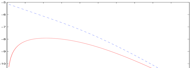
Figure 1: Interaction correction to the noise (solid line) and the ”naive expectation” (dashed line), see text for definitions.

5 Experimental Relevance

¿From the experimental point of view and for standard range of parameters, the effect we predict here is quite small (i.e., the logarithm of the ratio between the voltage and the temperature dominated corrections is typically close to unity. However, the incipient logarithmic singularity found here may, in principle, be spotted by carefully scanning the temperature dependence of the noise. Moreover, one can push the temperature and the voltage to values where the effect is particularly enhanced. Fig[1] presents a comparison of the corrections to the zero frequency current noise derived here (solid line) with a “naive” prediction (dashed line). The latter refers to using a standard expression for the shot noise, where we insert the non-equilibrium interaction corrections for $G_{Ohm}$. Here our two-dimensional metallic film is assumed to have a square geometry. Its conductance measured in units of quantum conductance is taken to be $G_{Ohm}=10\frac{e^{2}}{\hbar}$, and the value of the elastic mean free time is chosen to be $\tau=10^{-}2\frac{1}{meV}$. The applied bias $V=1meV$ and the temperature varies in the range $0.001{\rm meV}<kT<1{\rm meV}$. As the temperature decreases, the discrepancy between the ”naive expectation” and the correct result becomes increasingly pronounced.

References

- [1] Sh. Kogan Electronic Noise and Fluctuations in Solids , Cambridge Press (1996) .
- [2] Ya. M. Blanter, M. Büttiker Physics Reports 336, 2, (2000) .
- [3] M.J.M. de Jong and C.W.J. Beenakker in a Mesoscopic Electron Transport, NATO ASI Series E, Vol 345, Kluwer Academic Publishers, Dordrecht, (1997).
- [4] R. Landauer, 1989, private communication.
- [5] V.A. Khlus JETP 66 , 6 (1987) .
- [6] G. Lesovik JETP Lett., 49 , 592 (1989).
- [7] M. Büttiker Phys. Rev. Lett 65 , 2901 (1990) .
- [8] B.L. Altshuler, L. S. Levitov and A. Yu. Yakovetz JETP Lett. 59, 12 (1994) .
- [9] One should also keep in mind that this type of analysis is applicable only in the case when shot or Nyquist noise are dominant, and it is justified to neglect noise, i.e. the “zero frequency” is assumed to be finite.
- [10] C.W. Beenakker and M. Büttiker Phys. Rev. B 46, 1889 (1992).
- [11] Sh.M. Shulman A.Ya. Kogan JETP 29 , 3 (1969) .
- [12] K.E. Nagaev Phys. Rev. B 57, 4628 (1998) .
- [13] K.E. Nagaev Phys. Rev. B 62, 5066 (2000) .
- [14] Y. Naveh, D.V. Averin and K.K. Likharev . Phys. Rev. B 59, 2848, (1999);Y. Naveh, A.N. Korotkova and K.K. Likharev Phys. Rev. B (RC) 60, 2169 (1999) .
- [15] K.E. Nagaev Phys. Rev. B 52, 4740, (1995) .
- [16] A. H. Steinbach J. M. Martinis and M. H. Devoret em Phys. Rev. Lett. 76. 3806 (1996); M. Henny, S. Oberholzer, C. Strunk, and C. Sch nenberger Phys. Rev. B 59, 2871 (1999).
- [17] R de-Piccioto, M. Reznikov, M. Heiblum, V. Umansky, G. Bunin, D. Mahalu Nature 389, 6647 (1997), L. Saminadayar, D. C. Glattli, Y. Jin, B. Etienne . Phys.Rev. Lett. 79, 2526 (1997) .
- [18] B.L. Altshuler and A.G. Aronov in “Electron-Electron Interaction in Disordered Systems”, Elsevier Science Publishers B.V., Nort-Holand, New-York (1985) .
- [19] By this we do not imply that the system is at equilibrium.On the contrary, the distribution function of the electron gas is a weighted sum of two Fermi-Dirac functions, with different chemical potentials but the same underlying .
- [20] D.B. Gutman Y. Gefen , cond-mat/0102134
- [21] A. Kamenev, A. Andreev Phys. Rev. B 60, 2218 (1999).
- [22] A.M. Finkelstein “Electron Liquid in disordered Conductors” Sov. Sci. Rev. A. Phys. 14 Harwood Academic Publishers, GmbH, London (1990) .
- [23] C. Chamon, A.W. Ludwig, C. Nayak Phys. Rev. B 60, 2239 (1999) .
- [24] K.E. Nagaev Phys. Let. A 169, 103 (1992) .
- [25] The diffusion propagator D is defined through with the appropriate boundary conditions.
- [26] In order for the diffusion approximation for the kinetic equation to be valid , deviations from equilibrium should be small, i.e. the energy gain between two consecutive elastic scattering is small in comparison with the Fermi energy ( ) .
- [27] The subscript refers to averaging with respect to the non-interacting action.