Dynamical Monte Carlo Study of Equilibrium Polymers (II):
The Rôle of Rings
Abstract
We investigate by means of a number of different dynamical Monte Carlo simulation methods the self-assembly of equilibrium polymers in dilute, semidilute and concentrated solutions under good-solvent conditions. In our simulations, both linear chains and closed loops compete for the monomers, expanding on earlier work in which loop formation was disallowed. Our findings show that the conformational properties of the linear chains, as well as the shape of their size distribution function, are not altered by the formation of rings. Rings only seem to deplete material from the solution available to the linear chains. In agreement with scaling theory, the rings obey an algebraic size distribution, whereas the linear chains conform to a Schultz–Zimm type of distribution in dilute solution, and to an exponentional distribution in semidilute and concentrated solution. A diagram presenting different states of aggregation, including monomer-, ring- and chain-dominated regimes, is given. The relevance of our work in the context of experiment is discussed.
PACS numbers: 82.35.+t, 61.25H, 64.60C
I Introduction.
Solutions of highly elongated, cylindrical giant micelles are arguably among the best studied of the so-called equilibrium polymers [1]. Equilibrium polymers are formed in reversible polymerisation processes, and are in chemical equilibrium with each other, i.e., monomeric material is continually exchanged between the assemblies. An aspect not at all well understood is why ring closure seems to be unimportant in solutions of linear micelles, although this would remove unfavorable free ends (“end caps”) from the solution. Closed loops have been observed in electron microscopic images of giant micelles [2], but — as has been argued elsewhere [3, 4, 5] — in too low concentrations to significantly influence the properties of micellar systems. In other types of equilibrium polymer, such as liquid sulfur, the presence of rings is on the other hand thought to be all-important [6]. It is believed that rings are suppressed in those self-assembled polymeric systems that are sufficiently rigid on the scale of the individual monomers[3, 4, 5].
A useful model describing the self-assembly of giant micelles is what we call the Restricted Model of equilibrium polymers, where by definition ring closure and branching of chains are disallowed, and only linear chains form. In this model, the linear self-assembly is regulated by a free energy penalty associated with the free ends, the so-called end cap (free) energy . The end cap energy is normally presumed to be a constant independent of the chain size or aggregation number, , and of the overall monomer density [7]. The basic scaling predictions for the equilibrium polymerisation within the Restricted Model [3, 8, 9, 10] are based on classical polymer physics[11], and have been tested by two of us (JPW, AM) by means of various Monte Carlo approaches [12, 13, 14].
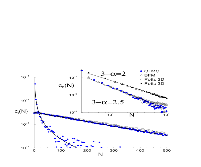
Despite their inherent polydispersity, self-assembled linear polymers resemble in many ways conventional polymers, that is, polymers with a fixed molecular weight. Indeed, the known statistical properties of conventional polymers have been applied quite successfully to predict the probability distribution function of the size of equilibrium polymers. In agreement with theoretical predictions [3], the size distribution function has for instance been shown to decay essentially exponentially with size in the semidilute and concentrated regimes, because then correlations generated by the excluded volume interaction are small [13]. A typical aggregate size distribution in a solution with strongly overlapping chains, obtained by computer simulation, is given in Fig. 1 (open squares).
In the present work we relax the no-loop constraint, and discuss systems of (mainly) flexible equilibrium polymers under good-solvent conditions, where linear chains have to compete with rings for the available monomers at given total density , and end cap energy . Branching of chains remains forbidden. We discuss in detail the number density of chains and rings of in different regimes (dilute versus strong overlap, ring versus chain dominated), and construct the complete “phase” diagram of this Unrestricted Model. Following up an an earlier, less extensive study [14], we report in this paper results obtained with a lattice-based Monte Carlo method[13, 15], and with a more recent off-lattice Monte Carlo scheme [14, 16]. We have succeeded in mapping the results of both methods onto each other, by making use of the natural length and energy scales that describe the configurations of the equilibrium polymers. This has enabled us to extract from the data the unknown prefactors that enter in the standard scaling theory, allowing us to construct a full diagram of states. Qualitatively, we confirm older, less elaborate descriptions [4, 5]. As can be seen in Fig. 1, the number density of rings as a function of aggregation number (indicated by the filled circles) is strongly singular, and dominated by a lower cut-off, that is, by the smallest ring allowed in the simulation. Effectively, this causes the crossover between dilute and semidilute regime, and that between ring- and chain-dominated regimes to coincide, at least for large end-cap energies .
This paper is organized as follows. We start in Sec. II with a brief presentation of the computational methods applied. Some technicalities concerning the parameters used and the configurations sampled are considered in Sec. III. The main computational results of this paper are presented in the Sections IV, VI and VII. In Sec. IV we discuss conformational properties, recall some notions and concepts of the physics of conventional polymers (of fixed size), and determine the size of the excluded volume blob [11]. The following three Sections V, VI and VII are dedicated to the mass distributions. In the short Sec. V we fix some notions, refine the problem and pose specific tasks. Subsequently, we discuss the number density of linear chains of size , , in Sec. VI. Results obtained within the Restricted Model (with rings suppressed) and the Unrestricted Model (with rings allowed) are compared. We attempt to map both Monte Carlo methods onto each other, and discuss the physics at extremely high densities, where our off-lattice Monte Carlo approach exhibits features linked to packing effects, not present in the lattice-based Monte Carlo method. The number density of rings of aggregation number , , and its connection to the size and mass distribution of the linear chains are discussed in Sec. VII – the core of the paper. In Sec. VIII we calculate the different regimes for systems of flexible equilibrium polymers in a good solvent, and compare this with the “measured” distribution of monomers over the rings and linear chains. In the final Sec. IX we summarize our findings, and speculate on the relevance of ring formation in some recent experiments [17, 18, 19].
II Algorithms.
All the computational algorithms we discuss are standard Monte Carlo schemes which have already been described and tested in depth in recent publications [12, 13, 14]. We shall therefore be extremely brief.
The first method which was introduced to simulate the equilibrium polymers within the Restricted Model, is a grand canonical lattice algorithm based on a mapping on a Potts model[12]. Because this model lives on a simple cubic lattice, closed loops are by geometry forced to consist of an even number of monomers. Results obtained with this model will only be briefly mentioned (in connection with Fig. 1). We discuss in more detail results obtained with two canonical Monte Carlo approaches — a lattice scheme [13] based on the Bond Fluctuation Model (BFM) [15], and a more recent off-lattice Monte Carlo (OLMC) approach [14] generalizing an efficient bead-spring model. All BFM and OLMC simulations have been done in three spatial dimensions, the Potts model simulations in two and three dimensions.
The BFM used in the present investigation is athermal, besides the constant scission energy , which characterizes the bonded interaction: an energy is released every time a bond forms. Apart from the no-overlap conditions modelling hard-core excluded volume interactions, no other bonded (such as a stiffness potential) or non-bonded interaction has been used in the present study, though they might be readily included.
In the off-lattice model, beads interact via a so-called (shifted) FENE potential for the bonded, and a purely repulsive Morse potential for the non-bonded interactions [16]. The bonded interaction
| (1) |
depends non-trivially on the distance between two monomers. Here, denotes again the constant part of the scission energy, and the spring constant. The former quantity will be related with the model-independent effective end-cap free energy , in Sec.VI. Note further that the FENE potential is harmonic near its minimum at , while exactly at , . The potential diverges logarithmically to infinity if and if , where and are the maximum and minimum extension of the spring. Following ref.[16], we set , and . Units are chosen such that .
Both models use local jump attempts. The time is measured, as usual, in Monte Carlo steps (MCS) per monomer. Every monomer is chosen at random, and allowed to perform a move subject to a Metropolis acceptance probability [13, 14]. In simulations the bonds between neighbors along the backbone of a chain are constantly subject to scission and recombination events. Since chains are only transient objects the data structure of the chains can only be based on the individual monomers, or, and this is the way we operate, on the notion of saturated and unsaturated bonds. An unsaturated bond does not connect a monomer to another one, a saturated bond does. Hence, we use no direct chain information, but lists of pointers linking up the bonds[13]. With a given frequency one of the bonds (saturated or unsaturated) is chosen at random. If that bond happens to be saturated an attempt is made to break it, if it is unsaturated, i.e., if the monomer is at the end of a chain or a free monomer, an attempt is made to create a bond with another monomer sufficiently close. Obviously, for reasons of detailed balance, the bond formed must come out of the same set or range of bonds out of which also scission events are allowed to take place [13, 14]. We do not allow for branching in the present study. The minimal length of a closed loop is , i.e. closed dimers are not permitted. Free monomers are also not allowed to self-saturate their two unsaturated bonds.
III Parameters and configurations.
The only two model parameters of operational relevance in the present study to tune the system properties are the scission energy and the number density . The starting configurations consist in both sets of simulations of randomly distributed and non-bonded monomers, which we cool down step by step (a sequence of so-called ‘T-Jumps’), each step sampling a higher scission energy up to a maximum . This was done in order to produce a sufficient chain length and concentration variation to be able to put to the test the theoretical scaling predictions.
Due to the constant breaking and recombining of the bonds, equilibration is much faster in our equilibrium polymeric system than is usually observed in systems of conventional polymers with fixed bonds. The algorithm presented above (using the pointer lists between bonds) allows us to simulate a large number of particles at very modest expenses of operational memory.
In our BFM simulations, we varied the number density over three orders of magnitude from ( monomers per box) to (containing monomers per box). For densities smaller than cubic lattices with volume were used, whilst for higher densities a smaller box sufficed of volume . Note that in the BFM every monomer consists of an elementary cube, whose eight sites on the cubic lattice are blocked for further occupation[15]. As a result of this, the volume fraction of material is given by . As was shown elsewhere[20, 21], volume fractions of around are already quite dense within the BFM. The reason is that at higher densities than this, the system turns glassy due to the blockage of neighboring sites by other monomers.
Most of the off-lattice Monte Carlo results involve particles for number densities between and (and appropriately chosen box sizes). Generally, we have sampled with the off-lattice Monte Carlo method more systems in the high and extremely high density regime, while we have explored with the BFM more systems in the dilute and semidilute regimes. Note that the highest densities in our off-lattice Monte Carlo simulations correspond to extraordinarily concentrated solutions. Indeed, if we estimate the corresponding volume fractions, we find that in our simulations these vary between and . (To obtain this estimate, an effective bead volume was used, with a measured mean bond length of .) The latter value of has to be compared with the (only slightly larger) hard-sphere freezing volume fraction (“Alder transition”) of about one half. Our simulations therefore extend to the “melt” regime of a dense liquid.
In passing we note that strictly speaking the mean bond length is not a constant, but decreases weakly with increasing density. However, this does not pose a serious problem, for we find that the total interaction energy per bond does remain roughly constant, with a for all overall monomer densities and scission energies probed.
Periodically, the whole system is examined and various moments and distributions, such as the number densities , are counted and stored. Here, and below, we refer to ring-related quantities by using a subscript , and to chain-related ones by a subscript . The number densities are normalized such that , with the overall density of monomers in species . Obviously, the sum of monomers in rings, , and that in linear chains, , is equal to the overall monomer density . (Free monomers are counted as linear chains of length .) Obviously, and in the Restricted Model, where rings are disallowed. We emphasize that the mean chain length remains always two orders of magnitudes smaller than the total particle number within the box. From our previous studies within the Restricted Model [13, 14], we expect finite box-size effects to be small.
Because of the differences in the lattice and off-lattice algorithms, we cannot expect the results obtained using these two methods to be directly comparable, even when the same parameters are used. To make a comparison possible, all relevant system parameters have to be mapped onto each other. This we do by taking the dilute limit as reference state. As the intrinsic energy scale we use , with a model-dependent shift parameter presented in Sec.VI. The intrinsic length scales are the mean bond length , and a length to be discussed in the next section.
IV Distributions of size.
Let us first discuss the conformational properties of equilibrium polymers, and show that not only they follow the same universal laws as conventional polymers, but also that there is no essential difference in the behaviour of linear chains in the Restricted and Unrestricted Models.
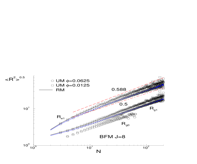
The configurational behaviour of the equilibrium polymers is most easily demonstrated by plotting their mean size as a function of the aggregation number , as is done in Fig.2. Indicated are the mean end-to-end distance of the linear chains, , and the radii of gyration of the chains and the rings, and . Averages have been taken over all linear chains () or rings () of given mass in the simulation box. Only results obtained with the bond fluctuation method are shown, for two different densities and a fixed value of the scission energy . Similar results have been obtained with the off-lattice Monte Carlo method. Symbols are used for the distributions from the self-assembled chains in the presence of rings, lines for those without rings. Despite the fact that the simulations point at the presence of a large number of rings within the Unrestricted Model, with the dilute systems even being ring dominated, there is no measurable difference between the results for the linear chain sizes in the Restricted and Unrestricted Model calculations. This we quite generally find for all densities probed, and within both simulation methods.
Indicated in the figure are two dashed lines, giving the theoretical slopes valid for very long polymers in dilute and concentrated solution [11]. In the dilute limit the chains are swollen and their size is described by the scaling relation , with a self-avoiding walk exponent of . Surprisingly, the relatively small rings shown in Fig.2 also closely follow the (asymptotic) scaling behaviour of their linear counterparts. In the following, the dilute limit will be used as reference state to be able to make a comparison between the different simulation models. As natural lengths we use the mean bond length and an effective bond length , the latter determined from a fit of the simulation data to the scaling relation . These two lengths in turn suggest a measure for the stiffness of the chains, which we shall call the “persistence length” of the chains, although obviously it is a dimensionless quantity. For the BFM we find [13], and for the off-lattice Monte Carlo method . In both cases this gives a persistence length that are of similar value (, for the BFM; , for off-lattice model). The found values for are essentially identical to what was obtained previously for monodisperse linear polymers [16, 21]. In a similar fashion, one may define and measure the prefactors and from the radii of gyration and . In line with our previous work on conventional polymers studied in [21], we find and . This result holds again for both simulation methods.
Figure 2 shows that, as expected[11], the excluded volume correlations in our equilibrium systems are screened out for strongly overlapping chains. More precisely, the chains become Gaussian chains of blobs of size , each blob containing monomers, with
| (2) |
and G an as yet unknown prefactor. The value of may be fixed using the classical definition for the crossover density of a monodisperse solution: . This definition gives for the prefactor , a value that turns out to be numerically consistent with alternative estimates obtained from fits to the scaling relations or .
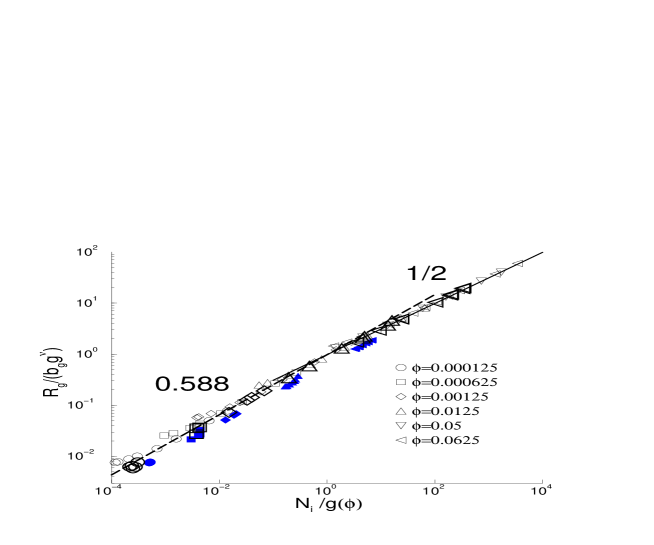
A further test of the configurational properties of the equilibrium polymers is provided by determining the dependence of the first moment of the size distributions on the mean aggregation number . Our results are presented in Fig.3, where we have plotted the radius of gyration divided by the blob size , versus the mean aggregation number divided by the number of monomers per blob . In order to calculate these reduced quantities, we used eq.(2) together with our previous estimate for . The figure shows that the mean chain sizes of the living polymers again follow the same universal master curve as conventional polymers [11]. Again we observe that the ring sizes, indicated by the full symbols, follow the same scaling law as the linear chains, which is actually rather surprising considering their relatively small size. The fact that the two slopes that indicate the scaling behaviour expected in the dilute and semidilute regimes cross nicely at , shows that our estimate of is actually rather accurate. Alternatively, we could have used this crossover point between the two regimes to define the prefactor .
In conclusion, the conformational properties of equilibrium chains are (within numerical accuracy) identical to those of polymers of fixed length. This is in contrast to earlier speculation in the literature, where it was surmised that rings might strongly influence the screening of excluded volume close to the crossover from the dilute to the semidilute regime[3]. We find that the universal functions are neither altered by the polydispersity, nor by the presence of rings. The blob size is a function of total monomer density only.
V Mass distributions of equilibrium polymers.
Next we turn our attention to the probabilities of finding aggregates of a certain aggregation number. For equilibrium polymers that are long compared to the effective bond length , the main departure from conventional theory of flexible polymer solutions is that the reversibility of the self-assembly process ensures that the degrees of polymerisation are in thermal equilibrium. This means that the distributions and are not fixed, but minimize the thermodynamic potential of the system. It is natural to attempt a simplified theoretical description, using a Flory-Huggins type of mean-field approximation
| (3) |
where we have written the thermodynamic potential as a sum over the different species for rings and for linear chains, and over all possible aggregation numbers . The factor in the logarithm enters for dimensional reasons, where we set equal to the mean bond length of the chains in the dilute regime; all energy units are measured in units of thermal energy, . This ansatz for the thermodynamic potential is strongly motivated by its success describing the properties of equilibrium polymers within the Restricted Model, where ring formation is suppressed [13, 14]. The first term on the right is the usual translational entropy. The second term represents a Lagrange multiplier or chemical potential which fixes the total monomer density . All contributions to the free energy which are extensive or linear in are absorbed in this Lagrange multiplier. The as yet not specified terms describe the free energy contributions not extensive in the degree of polymerisation of the rings and linear chains. In general these may depend on the interactions between different chains and chain parts, and as a rule differ in the dilute, semidilute and melt regimes. We stress that in the prescription of eq. (3) terms (such as virial terms) which are not conjugate to or need not be made explicit, as they are absorbed in . Inspired by the results of the previous section, the central assumption of eq. (3) is that the two distribution functions are only coupled via the chemical potential that makes sure that the total amount of monomers is conserved.
In equilibrium, the distribution functions functionally minimise the thermodynamic potential, , giving
| (4) | |||||
| (5) |
where we set and for convenience. The free energy associated with the linear chains is split into a model- and density-invariant end-cap free energy (containing the operational scission energy and a shift factor discussed below), and a remaining part that somehow describes excluded volume correlations [11]. The Heaviside function enforces a smallest possible ring , in effect a lower cut-off. In actual systems this cut-off may depend on factors such as the detailed chemistry of the equilibrium polymers in hand, and on their bending stiffness not explicitly modelled here.
Before we are able to comprehensively analyse our computer simulation results aided by eq. (5), our task is (1) to complete the mapping of the simulation methods already started in the previous section, (2) to show that the Flory-Huggins ansatz is indeed justified, and that the ring and chain distributions decouple, (3) to identify the free energy terms and , (4) to show that the are only functions of and the total density as indicated, and (5) to determine the equilibrium values of , and for a given system . In the next two sections VI and VII we consider the distribution functions of the linear chains and rings, and analyse the free energy terms (tasks 3 and 4). The mapping (task 1) will be completed in Sec. VI B, where we relate the natural (and in principle measurable) energy scale with the operational parameter . We show there that the distribution functions of linear chains in the Unrestricted Model can be computed from those in the Restricted Model, if the density of monomers in chains is given (task 2). In Sec. VI E we study the density crossover scaling for . The relative distribution of monomers in rings and in linear chains (task 5) will be considered in Sec. VIII.
VI Mass distributions of linear chains.
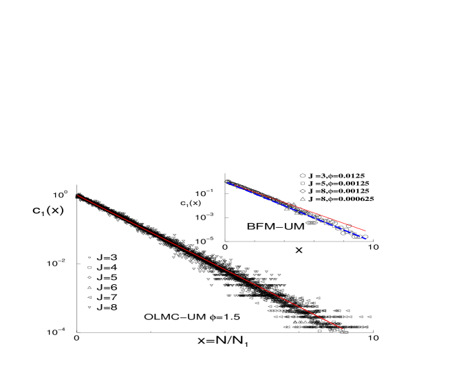
In this section we focus attention on the size distributions of the linear equilibrium polymers, as determined by computer simulation, within both the Restricted and Unrestricted Model settings. A typical example is given in Fig.1, where results are shown obtained with the off-lattice algorithm at high densities, that is, in the limit of strongly overlapping chains (). The distribution functions for the Restricted and Unrestricted Models are both to high accuracy pure exponentials. Under conditions where linear chains dominate in the Unrestricted Model (), we find that results from the Restricted and Unrestricted Models converge systematically. This is generally true in the limit of strongly overlapping equilibrium polymers, because then linear chains dominate the population of equilibrium polymers. (See also below.) At variance with recently published results of a simulation study [22], we do not observe any sign of an algebraic singularity in the distribution function of the linear chains, even at the extremely high volume fraction of . Results (not shown) from the BFM simulations confirm all trends observed with the off-lattice Monte Carlo treatment.
A more critical test of our statement that rings only marginally influence the distribution functions of the linear chains is provided in Fig.4, we have plotted the distribution of linear chains against the natural scaling variable . Apparently, in the regime of strongly overlapping chains (main figure) the data collapse onto for a whole host of scission energies . (Note that chain statistics deteriorate in the tail of the distribution.) In the dilute limit we find a similar data collapse, but with slightly different slope, pointing at a distribution of the type , with a constant identified below as a critical exponent. See the inset of figure 4, where results obtained from the BFM simulations covering the dilute limit are shown. Identical distributions have been found in both limits for systems without rings [13, 14].
How can our observations be understood? We have demonstrated in a previous publication that within the Restricted Model, the free energy term in the expression for the distribution function of linear chains in eq. (5) can be calculated from the scaling theory of conventional polymers in a good solvent [11]. Agreement with simulation data turned out to be remarkably good [13, 14]. We show here that this ansatz is also justified when rings are present, as long as the overall monomer density is not extremely high (Sec. VI D).
A The Mean-Field solvent.
Starting with the (hypothetical) conditions where mean-field type of behaviour dictates the distribution functions, is a constant. may then be absorbed in , i.e., in that case we may simply put . From eq. (5) we thus read off that within mean-field theory, the distribution function must be a pure exponential . It is easily shown that for this type of distribution, the equality holds, albeit exactly only in the limit of large mean aggregation numbers . For the mean-chain length we obtain
| (6) |
with an amplitude and mean-field exponents . Note that in the Unrestricted Model is a function of , and only indirectly dependent on the control parameter .
B The dilute limit.
Although largely unimportant in the semi-dilute and concentrated regimes, correlation effects do matter in the dilute regime, as we have in fact already seen in our discussion of the conformational properties in Sec. IV. Using the known statistical properties of self-avoiding walks, we infer that the free energy of a chain decreases logarithmically with the degree of polymerisation [11]
| (7) |
where is the susceptibility exponent of the vector model in 3 spatial dimensions[23]. Eq. (7) leads to a Schultz-Zimm distribution for the linear chains
| (8) |
which indeed is born out by our simulation results, presented in the inset of Fig. 4 [24], since in the dilute limit we have provided [3, 13].
As already advertised in the previous section, we use the simulation results obtained in the dilute limit to map the different simulation models onto each other. The natural energy scale is established by fitting the data for to eq. (8), using the equality . Having done this for the Restricted and Unrestricted Model simulation at various values of and , we find for the BFM and for off-lattice model. We stress that is model dependent, absorbing the different physical behaviour of the models on a microscopic scale (see Sec.II). It can only be coincidental that for the models we used the ’s turn out to be almost identical. Whatever the reason, the fixing of completes the mapping.
The concentration dependence of the mean aggregation number in the dilute regime, for future reference denoted by , is given by
| (9) |
with the exponents , and a prefactor , in terms of the exponent and the usual gamma function . Our simulations confirm these exponents and the prefactor (results not shown).
C Semidilute solutions.
The aggregation number dependent free energy contribution eq. (7) describes only dilute chains, i.e., chains which are too short to overlap. From the standard theory of conventional polymers [11], one expects excluded volume effects to be screened out when the chains strongly overlap. Even then, this happens only for chains larger than the blob size, that is, for aggregation numbers , where levels off to
| (10) |
and ; the quantity scales like (see eq. 2), but with the different prefactor
| (11) |
fixed by a constant , estimated below.
That indeed switches from length dependent (dilute) to density dependent (semidilute and melt) is shown in Fig. 5, where we plot measured values of , using the mean-field relation and . Figure 5 shows that is a constant of the degree of polymerisation at high overlap concentrations [25], as it should. It explains the scaling relation observed in Fig. 4, not least because the values of found for the Restricted and Unrestricted Models turn out to be identical if the overlap is strong enough. At low densities (), becomes dependent on the chain length, due to the unscreened excluded volume interactions, but also on whether in the model ring formation is allowed or not. In the Unrestricted Model ring formation is allowed, and as a result of that some of the available material is stored in rings. This causes a shift in the distribution of linear chains relative to that in the Restricted Model. The trends of figure 4 confirm this.
Using the measured plateau values of , we verify that the density variation predicted by eq. (10) holds, and estimate the prefactor via eq. (11). This is done in Fig. 6, where we have plotted the plateau values versus the dimensionless overall concentration of monomer, . Data from the BFM (pluses) and the OLMC (asterisks) are included in the figure. Also shown are values as they may be measured via the mean aggregation number in the strong overlap limit (SOL), that is, in semidilute and concentrated solution
| (12) |
which depends explicitly on both and . We use the directly measured and to obtain . This procedure gives identical results as the obtained straight from the distribution functions. Again, there is no observable difference between the results obtained with and without ring formation. In line with the prediction of eq. (10 ), we find a logarithmic density dependence (dashed line) with a prefactor . That in the semidilute regime both off-lattice and BFM results coincide reinforces our belief that the mapping between the models is robust. The divergence of the lattice and off-lattice data at very high densities is not problematic. A discussion of this issue we postpone to Sec. VI D.
Within the semidilute regime, i.e., within the validity of eq. (10), the mean degree of polymerisation of the linear chains is power law function of and , and may be brought under the generic form of eq. (6)
| (13) |
with , , and an amplitude
| (14) |
with . The (very weak) -dependence arises because depends on rather than on . Note that in the limit of linear chain dominance ( ) one recovers the density dependence of the Restricted Model, i.e., [3, 13]. We verified the validity of eqs. (13) and (14) by comparison with the computer simulation data, but do not pause here to elaborate on the details. In Sec. VI E we present the full crossover scaling of covering the entire range of concentrations from the dilute to the melt regime.
D Concentrated solutions.
As we have discussed in a previous paper on the equilibrium polymerisation in the absence of ring formation [14], eq. (13) only holds within the semidilute regime. This implies that there must be a large number of monomers within a blob, for otherwise the blob concept becomes meaningless. Within our off-lattice Monte Carlo approach, we have probed such high densities that the semidilute description does break down – this is the melt regime already alluded to. It appears that we enter the melt regime if , where a different physical behaviour intervenes, essentially due to fluid-like correlations resulting from local packing constraints. Clearly, effects of this nature cannot be expected to arise in any lattice-based bond fluctuation technique, because of the presence of an underlying lattice structure suppresses to a great extent fluid-like correlations.
Our off-lattice Monte Carlo simulations point at a linear relationship between and the concentration material upon entering the melt regime: with and . See Fig. 6, and in particular the inset. This also clearly shows that within the lattice model, the semidilute regime extends deeply into the melt regime, that is, even for concentrations where the blobs are so small as to contain no more than monomers. We attribute this to the lack of a true fluid structure in the lattice-based model.
We conclude from the above that while eq. (10) breaks down in the melt, eq. (12) still holds (see Sec. VI E below). and are then no longer related via a pure power law, but in addition via an exponential enhancement term: . Direct measurement of in our simulations confirms this once more. Indications for the deviation from the usual power-law behaviour at very high densities have in fact also been found in earlier simulation studies [22, 26]. The precise reason for the emergence of the exponential correction is at this point difficult to give. Theoretically, exponential corrections of the sort found here have been predicted theoretically for rigid and semiflexible micelles, but only within a second virial theory valid at low densities [27]. Within the second virial theory, the exponential density dependence of arises from excluded volume interactions between the free ends and the central parts of the chains. Clearly, although the applicability of the concepts advanced in [27] to our high density system of flexible bead-spring chains is dubious, one may surmise that differences in the packing of the central beads and those near the ends of the chains could well lie at the root of problem. Further study is definitely warranted.
E Crossover scaling of the mean length of the linear chains.
In this subsection we discuss the crossover scaling behaviour for the linear chain aggregation number , focusing on the -exponent (Fig. 7) and on the -exponent (Fig. 8). We show that the computer simulation data from both Restricted and Unrestricted Models collapse onto the same universal function, if properly rescaled, and the directly measured density is used. Again we include data from both the bond fluctuation model (BFM) and the off-lattice Monte Carlo (OLMC) method. Results from the latter technique have been shifted upwards for reasons of clarity in both the figures 7 and 8.
In Fig. 7 we compare the actual, measured with a “hypothetical” dilute mean chain length calculated from eq. (9). In the dilute regime , but outside this regime represents an extrapolated value. Plotted is not against , but the quantity against the quantity , specifically chosen to get a scaling with the -exponent: . Here, is the mean chain length at the crossover density from the dilute to the strongly overlapping regime, defined by the equality . Equating eqs. (9) and (12), gives for this quantity
| (15) |
In the semidilute regime becomes proportional to , with an amplitude very close to the blob prefactor . Because of the very large exponent , we regard these two values as numerically identical. Our conclusion is that represents a generalization of the number of monomers per blob , also valid in the limit of very high densities where eq. (10) does no longer apply. In passing we also note that is also consistent with (cf. eqs. (14) and (11)). In other words, our characterisation of the excluded-volume blob is internally consistent.
The purpose of all this is to make clear that in the high density regime discussed in the previous section, the mean aggregation number can be described by the same universal function that is valid in the dilute and semidilute regimes, if the notion of the number of monomers per blob is generalised appropriately. The function that describes the generalised blob is universal in the sense that it depends solely on the overall monomer density , and on the number of monomers per effective step length . Indeed, the data points obtained for the Restricted and Unrestricted Models, within the bond fluctuation and off-lattice Monte Carlo methods, all collapse on the same universal function. The scaling plot confirms the scaling relation we set out to investigate , with in the dilute limit, and in the semidilute and melt limits.
In our second scaling plot, Fig. 8, we show the effects of a density variation on . To focus on the concentration behaviour of the critical exponent , we make use of eqs. (9) and (13), and plot versus where , and and are known critical exponents. This should yield a scaling relation . Equating equations (9) and (13) gives a crossover density and a crossover length . The amplitudes and are determined from and , exactly as in the case of the Restricted Model, where [13]. The estimates cannot be expected to be very accurate because of the large exponent , but are consistent with the estimates obtained by using the amplitudes and predicted from (and/or .)
The data points for the dilute and semidilute regimes clearly collapse. As discussed earlier in the context of Fig.6, the off-lattice Monte Carlo data do not conform to the scaling theory at very high densities, due to the effects of packing that dominate the melt regime.
VII Mass distributions of closed loops.
It has become clear from the discussion of Sec. IV, that the dimensions of the linear equilibrium polymers are successfully described in terms of the Flory exponent . In the preceding Sec. VI we demonstrated that another critical exponent, the susceptibility exponent , is the exponent relevant to the description of the length distribution of the linear chains in the dilute and semidilute regimes. The length distribution of rings, only formed in the Unrestricted Model, is dominated by yet another critical exponent, . This exponent is the well-known specific heat exponent, related to the Flory exponent via the hyperscaling relation in spatial dimensions. As we shall make plausible below, the ring distribution is quite accurately described by the quasi singular scaling relation .
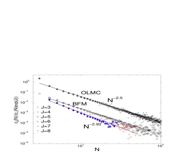
Let us return to main Fig. 1. The distribution of rings indeed follows a power law distribution with an in the dense limit of the off-lattice Monte Carlo simulation. This we expect, because in the dense limit and the simulation was done in . The hyperscaling relation is checked extensively in the inset of the figure, where we plot the distributions as obtained for not only by means of the off-lattice and bond fluctuation methods, but also from the grand-canonical Potts model simulations, mentioned in Sec. II. Also included are data from the Potts model in two dimensions, where . Because the Flory exponent is for the concentrated or melt regime in both two and three dimensions, our results confirm the hyperscaling relation.
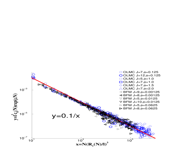
The strong power law behavior seen in Fig. 1 does not exclude an additional exponential damping, which we expect to be present from eq. (5). In the strong overlap regime this exponential damping is difficult to detect, because there is very small. However, the exponential damping of the ring distribution is observable in the dilute regime, as is made clear by Fig. 9. In the figure we present data from the off-lattice simulations, for different scission energies and at a fixed concentration . Note that increases with , as does (see Sec. VI B). For large values of we recover the power law behavior seen in Fig. 1, albeit with a different exponent because interactions are now not screened. This value is again in line with the hyperscaling relation, since in the dilute regime the Flory exponent obeys . The drawn lines are fits eq. (17).
If the properties of rings and linear chains really decouple as was assumed in our Flory-Huggins ansatz, we can measure the free energy difference between rings and linear chains directly by plotting the ratio
| (16) |
versus the aggregation number . This is done in Fig. 10, where we present off-lattice Monte Carlo data taken at a density of , and BFM data at (middle curve), the former shifted vertically for reasons of clarity. Both densities are in the strong overlap regime. The lowest curve gives BFM data, taken at the dilute densities (open symbols) and (filled symbols). The lines indicate power laws . From what we have said above about , we expect in the dilute limit, and in the strong-overlap limit. The Monte Carlo data confirm this expectation, demonstrating once more the validity of the Flory-Huggins ansatz (task 2).
Let us now briefly pause at a simple argument due to Porte, by which one may derive an expression for the ring distribution, and arrive at the exponent [4]. The ratio of the ring and linear chain distribution functions, eq. (16), must be equal to the ratio of the respective partition functions, which in turn must proportional to the probability of opening a loop. The probability of opening a loop is proportional to (i) the Boltzmann weight to break a single bond[28], (ii) the number of places where the ring can break, , and (iii) the volume that two neighboring segments can explore after being disconnected. Hence,
| (17) |
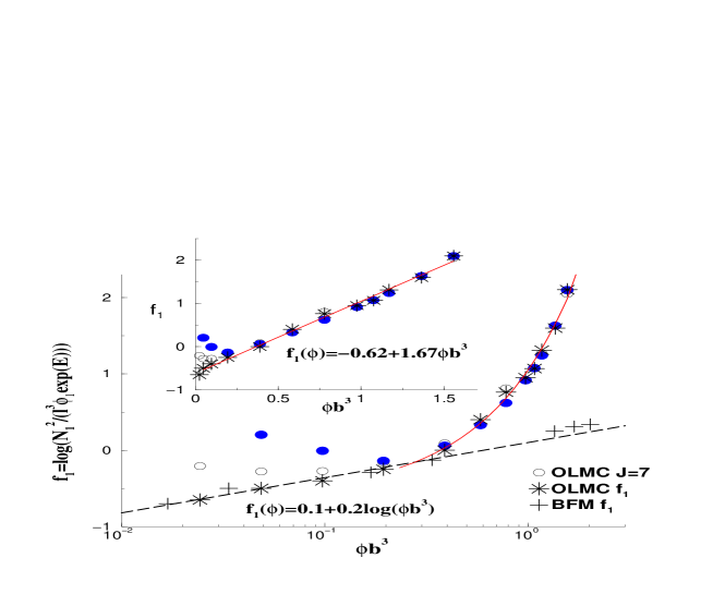
with an unknown constant of proportionality. We have put eq. (17) to the test in Fig. 11, using the directly measured end-to-end distance discussed in Sec. IV, and the measured chemical potential , as discussed in Sec. VI. A wealth of data from both the lattice-based and off-lattice Monte Carlo methods in various regimes is included in the figure. The collapse of the data is next to perfect – the main result of this paper. The non-trivial behaviour of in the dilute and semidilute regimes explains the complex density dependence of the ring distribution in the various concentration regimes. The scaling plot yields a value of for the constant of proportionality (Fig. 9), similar to the one estimated by Pfeuty and co-workers[6] in their analysis of self-assembled chains.
While the scaling relation eq. (17) appears to be well satisfied for relatively large , strong deviations from the universal asymptotic behavior is observed for small . As seen from inspection of, e.g., Fig. 9 or Fig. 10, an unexpectedly large number of trimer rings are present in our simulations. This is emphasized in Fig. 12, where we give the fraction of monomers trimer rings relative to the total amount, and to that in all the rings, as function of the overall concentration of aggregating material. At densities below most of all monomers are contained in trimers! The fraction of trimer rings seems largely independent of .
The effects of small chain length are systematically analyzed in Fig. (13), where we compare the measured free energy with the asymptotic behavior , valid for large . Here, is a constant function of , although it does depend on , because of the density dependence in the SOL. The density dependence shown in the inset, points at a decreasing tendency to form small rings with increasing concentration . It appears that the effect is much stronger in the off-lattice simulations than in the lattice-based approach, which reaches the asymptotic limit more rapidly (results not shown).
It is important to emphasize that the observed small-ring behaviour is not in contradiction with the scaling picture presented in Fig. 11. It is in part caused by the similar deviation from the asymptotic behaviour of the dimensions of short linear chains, as can be seen in Fig. 2. We find that short chains are smaller in dimension than expected from the scaling behaviour for large . As the entropy gain of opening a ring is smaller the shorter the chain, short rings become as a result of this more likely than expected. (See eq. (17).) In other words, the deviation from the asymptotic behavior of at small is caused (at least in part) by the small- behaviour of the dimensions of the linear chains.
That there are deviations from the universal asymptotic behavior in the small-ring population does not really come as a surprise. Unfortunately, even seemingly small shifts in the distribution of rings do matter when it comes to determining the relative amounts of rings and linear chains: the essentially algebraic distribution forces most of the ring mass to be concentrated in the smallest rings — exactly where the universal description based on scaling laws becomes inaccurate. This is the reason why obtaining a universal diagram of states based on theoretical argument, attempted in the next section, is fraught with difficulty, at least in principle. However, for the purpose of getting a qualitative picture of the aggregated states of equilibrium polymers, scaling theory provides a sufficiently accurate basis.
VIII Diagram of states.
If we accept the theoretical distributions of eq. (5) at face value, and augment these with the values for the parameters , , , , and obtained by fitting to the results of our computer simulations, we can calculate a diagram of states or “phase diagram” for our system of flexible equilibrium polymers [29]. For this purpose, we calculate, using eq. (5), the overall densities of monomers in rings and in linear chains, and , as well as the mean chain lengths, and , as a function of the total monomer density , and of the end cap energy . For the mean end-to-end distance , and the free energy correction to create an additional chain end, we simply put
| (18) | |||||
| (19) |
with the monomer number per blob and . Obviously, eq. (19) is only an approximation to the full universal functions.
The set of equations to be solved require a numerical evaluation, essentially because the sums cannot all be evaluated analytically. For a given we vary the Lagrange multiplier , and obtain from eq.(5) the densities , and, therefore, also . A complication is that the distribution functions themselves depend explicitly on the density , at least in the semidilute regime. The total density is of course not known a priori, and has to be evaluated for any given value of . In principle, the only way out is a recursive iterative scheme. Fortunately, matters become simplified significantly if one starts the calculation in the dilute regime (at large ) where both and are density independent. Recursive iteration may then be circumvented by slowly decreasing the value of , updating and , and then using a forward scheme to determine the next -value.
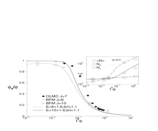
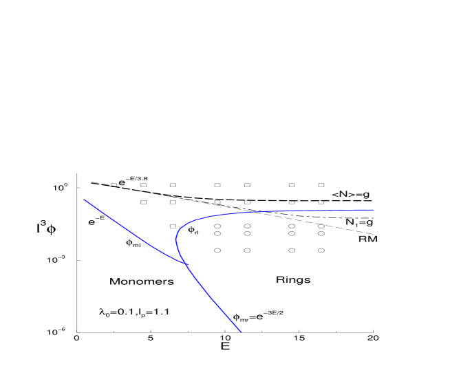
We first consider the relative distribution of the monomers over the rings and the linear chains in flexible equilibrium polymers, where we set the lower ring cut-off at , conform our simulations. In Fig. 14 we compare the concentration dependence of the fraction of monomers in rings, , as obtained from our simulation studies, with the numerical results of the idealized model defined above. In the inset we furthermore give the concentration dependence of the mean chain lengths , and . Considering that no additional fit parameters were used, the agreement, although not perfect, is actually quite reasonable. The general trend is well described by the model calculation.
The full diagram of states is presented in Fig. 15. We distinguish three regimes in the -plane: (i) one where free monomers dominate at low densities and end-cap energies, (ii) one where rings dominate, at intermediate densities and high end-cap energies, and (iii) one where linear chain dominate, at high densities. The crossover to the ring-dominated regime is defined by the equality . For energies larger than , we find two roots: the concentration demarcating the crossover between ring and linear chain dominance, and the concentration separating the monomer- and ring-dominated regimes. The crossover concentration is defined as that concentration when half the linear chains is in monomeric form, and half in polymeric form of . For comparison we have also indicated in Fig. 15 data found by means of computer simulation within the BFM. Configurations with ring dominance are denoted by circles, systems where linear chains dominate by squares. Apparently, the simulation data corroborate our theoretical phase diagram.
In the figure 15 we have in addition drawn the three dilute-semidilute crossover densities of relevance to our discussion. The thin dashed line denotes the crossover density , valid within the Restricted Model (where rings are absent). The presence of rings alters qualitatively the crossover density, for in the Unrestricted Model it becomes independent of at large end-cap energies. This bounds the semidilute regime to relatively high densities in the Unrestricted Model, as was in fact already remarked by Cates [3]. See Fig. 15. The semidilute regime cannot extend itself deeply into the ring regime, basically because the rings are too short. This is shown by the dashed-dotted line, which indicates the crossover density for the linear chains, as defined by equating with . (This definition of corresponds to the one given in Sec. VI.) Note that , and that the chains start to overlap slightly below the -line. The rings shorter than remain swollen at densities well above . This can be seen from the thick dashed line, the crossover density calculated by equating with the mean chain length of all chains (chains and rings). This crossover density has an asymptotic value in the limit of large end-cap energies. Around the crossover from the ring- to the linear chain-dominated regime, the mean chain length grows rapidly from to , because then most (but not all) of the additional monomers are now included in the long chains.
IX Discussion and Conclusions.
Based on extensive computer simulations in two and three dimensions, using a number of different simulational techniques, we conclude that the configurational properties of the self-assembled linear chains are not altered if ring closure is allowed. The same can be said about the shape of the probability distribution of the linear chains. We find that the probability of finding linear chains of a certain length drops off exponentially with length, at least for concentrations where the chains strongly overlap. In dilute solution, where the chains do not overlap, the distribution function is of the Schultz-Zimm form. Previously, the same distribution functions were found theoretically, as well as by means of computer simulations, in equilibrium polymerising systems where ring closure was suppressed. Is ring closure allowed, we find the resulting distribution of rings to be essentially algebraic, albeit that in dilute solution the algebraic distribution is dampened an additional exponential length dependence.
It seems that the rings formed in equilibrium polymerisation merely deplete monomers from solution, making fewer of them available for absorption into linear chains. This is experimentally relevant, because it shifts the crossover to the semidilute regime to significantly higher densities. Interestingly, of the amount of material present in the rings, a very large fraction resides in the smallest rings allowed – in fact much more so than expected from the universal scaling relations which seem to be valid for large enough rings. In our case the smallest rings possible are determined by an arbitrary cut-off. In reality, the smallest possible ring is likely to be determined by the chemistry of the system in hand, making the cut-off a non-universal quantity. An important factor determining the minimum size of a ring may well be the rigidity of the bonds connecting the basic building blocks of the equilibrium polymers, and possibly also the configurational properties of the building blocks themselves.
It has been argued in the literature that rings shorter than roughly a persistence length are highly unlikely to form[4, 5]. If it takes many monomers to make one persistence length, ring closure is suppressed in favour of linear chains. This might be the reason why rings seem to be unimportant in giant micellar systems, because each individual surfactant molecule does not contribute a great deal to the length of an aggregate. For giant micelles the number of monomers required to grow an aggregate the size of a persistence length may be very large indeed, even when the aggregate is quite flexible. The same need not be true in other types of equilibrium polymerising system, and for these ring formation must be relevant. Indeed, it is well known that in liquid sulfur rings play an important role. We speculate that the short S8 rings, which seem to overwhelmingly dominate the ring regime of liquid sulfur, represent the aforementioned lower cut-off.
The question arises why the problem of ring closure has not provoked a great deal of interest, for instance in relation to other types of equilibrium polymeric solutions. A plausible reason is that it appears to be difficult to experimentally distinguish between rings and linear chains, although new experimental techniques may change this in the future. Meijer and co-workers have recently been able to distinguish by means of NMR methods between material in tight rings and that in other chains in their system of hydrogen-bonded equilibrium polymers[18]. Unfortunately, these authors have not yet undertaken any systematic studies of the ring formation, for the moment barring a comparison with our computer simulation results.
Direct measurements of entire size distributions are also extremely rare in the field of equilibrium polymeric systems. In fact, we know of only a single study that has been published in the literature. Greer and co-workers quite recently presented size distributions of the living polymerisation of poly in the solvent tetrahydrofuran[19]. The distributions were obtained by means of size exclusion chromatography after termination of the polymerisation. The data very clearly show a distribution that is algebraic for small degrees of polymerisation, crossing over to an exponential distribution for large degrees of polymerisation, pointing at the presence of small rings. (The experiments cannot distinguish been rings and linear chains, so the distribution contains the sum of contributions from linear chains and rings, if present.) A mean-field power-law distribution proportional to turns out to fit the data quite well at low degrees of polymerisation.
We are somewhat puzzled by the good agreement with the (mean-field) prediction, for the equilibrium polymerisation reaction is initiated by sodium naphthalene. This initiator forms bifunctionally reactive polymeric anions, which in principle do not allow for a ring closure reaction. However, there are several mechanisms by which rings may form regardless. One mechanism is that of Coulombic association of the charged end groups. This is possible because of the presumably strong binding or localisation of the cationic counterions to the anionic end groups, the solvent being very hostile to charged species. The resulting effectively dipolar chain ends may themselves form larger clusters (dimers, trimers etc.) for the same reason, allowing in principle for all kinds associations, including rings. Another mechanism could be the presence of small amounts of oxygen, which in the termination reaction lead to the formation of polymer radicals which could close up. Even if rings are indeed formed in the living polymerisation studied by Greer, we feel a direct comparison with our simulations is not warranted. The reason is that these rings must then be formed by processed competing with the on-going linear anionic polymerisation, requiring a different model altogether.
Acknowledgments
This research has been supported by the Bulgarian National Foundation for Science and Research under Grant No. X-644/1996. JPW thanks M.E. Cates for helpful comments and hospitality in Edinburgh.
REFERENCES
- [1] The physical properties of EP and specifically GM have been reviewed briefly in [13] and more extensively in ref. [3]. In ref.[13] and [14] we also review and analyze some of the older computational work on EP.
- [2] T.M. Clausen, P.K. Vinson, J.R. Minter, H.T. Davis, Y. Talmon and W.G. Miller, J.Phys.Chem., 96, 474 (1992).
- [3] M. E. Cates and S. J. Candau, J. Phys. Cond. Matt. 2, 6869 (1990).
- [4] Porte G., in Micelles, Membranes, Microemulsions, and Monolayers, edited by W.M. Gelbart, A. Ben-Shaul and D.Roux (Springer-Verlag, New York) 1994.
- [5] P. van der Schoot, J. P. Wittmer, Macromolecular Theory and Simulations, 8, 428 (1999); cond-mat/9808175.
- [6] R.G. Petschek, P. Pfeuty and J.C. Wheeler, Phys. Rev. A, 34, 2391 (1986).
- [7] In the surfactant literature[3] giant micelles are often referred to as “living polymers” although this is potentially confusing since they are distinct from systems that reversibly polymerize stepwise, in the presence of an imposed density of initiators, for which this term has previously been reserved (see e.g. M. Szwarc, Nature, 178, 1168 (1956)). These classical living polymers polymerize (above or below some critical temperature) by addition of monomers on active chain ends. They are held together by strong covalent carbon-to-carbon bonds. For a recent review see S. C. Greer, Advances in Chemical Physics 96, 261 (1996).
- [8] P. van der Schoot, Europhys. Lett. 39, 25 (1997).
- [9] S.J. Kennedy and J.C. Wheeler, J.Phys. Chem. 78, 953 (1984).
- [10] L. Schäfer, Phys. Rev. B, 46, 6061 (1992).
- [11] P.G. de Gennes, Scaling Concepts in Polymer Physics, Cornell Univ. Press, Ithaca (1979); J. des Cloizeaux and G. Jannink, Polymers in Solution, Clarendon Oxford (1990).
- [12] A. Milchev and D. P. Landau, Phys. Rev. E 52, 6431 (1995).
- [13] J. P. Wittmer, A. Milchev, and M. E. Cates, J.Chem. Phys., 109, 834 (1998).
- [14] A. Milchev, J. P. Wittmer, D. Landau, Phys. Rev. E 61, 2959 (2000).
- [15] I. Carmesin and K. Kremer, Macromolecules, 21, 2819 (1988).
- [16] I. Gerroff, A. Milchev, W. Paul, and K. Binder, J. Phys. Chem. 98, 6526 (1993); A. Milchev, W. Paul, and K. Binder, J. Phys. Chem. 99, 4786 (1993).
- [17] P.Schurtenberger, C.Cavaco, F.Tilberg, and O.Regev, Langmuir, 12, 2894 (1996); G. Jerke, J.S. Pedersen, S.U. Egelhaaf, P. Schurtenberger, Phys. Rev. E, 56, 5772 (1997).
- [18] B.J.B. Folmer, R.P. Sijbesma and E.W. Meijer, Ang. Chem., submitted.
- [19] S. Sarkar Das, J. Zhuang, A. Ploplis Andrews, S.C. Greer, C.M. Guttman and W. Blair, J. Chem.Phys. 111, 9406 (1999).
- [20] W. Paul, K. Binder, D. Herrmann, and K. Kremer, J. Chem. Phys. 95, 7726 (1991).
- [21] M. Müller, J.P. Wittmer, M.E. Cates, Phys. Rev. E, 61, 4078 (2000).
- [22] Y. Rouault, Phys. Rev. E, 58, 6155 (1998).
- [23] S. Caracciolo, M.S. Causo, A. Pelissetto, Phys. Rev. E, 57, R1215 (1998).
- [24] Note that the -exponent for is only slightly larger than its mean-field vlue . Hence, the predicted power law depletion in the probability distributions for small is very weak and requires a relatively large mean mass at low densities to be seen. This is why within the range of the parameters accessible essentially only the tail is visible.
- [25] This finding is at variance to Gujrati (P.D. Gujrati, Phys. Rev. B 40, 5140 (1989)) according to whom the Schultz distribution eq. (8) holds independently of the overlap. It has been argued that corrections may arise to eq. (10) for the small fraction of chains that are too long for their excluded-volume interactions to be screened by the surrounding chains (under melt conditions this applies [11] to those chains whose length exceeds ). However, these contributions are exponentially small and can be neglected.
- [26] M. Kröger and R.Makhloufi, Phys. Rev. E 53, 2531 (1996).
- [27] P. van der Schoot and M. E. Cates, Langmuir 10, 670(1994); P. van der Schoot, J.Chem.Phys. 104, 1130 (1996).
- [28] Note the cancellation of the Boltzmann weight occurring on both sides of this equation. Hence, is independent on both and , i.e. on the specific model hamiltonian describing, e.g., the chain rigidity influencing both terms. This was not appropriately seen by two of us (PvS,JPW)[5].
- [29] It has to be stressed that “phase” means here “regime” rather than thermodynamic distinct phases associated with discontinuities in the free energy of the system. The transitions between different regimes only foreshadow the true thermodynamic phase transition at infinite end cap energies.