Interface fluctuations in disordered systems:
Universality and non-Gaussian statistics

Abstract

We employ a functional renormalization group to study interfaces in the presence of a pinning potential in $d=4-\epsilon$ dimensions. In contrast to a previous approach [D.S. Fisher, Phys. Rev. Lett. 56, 1964 (1986)] we use a soft-cutoff scheme. With the method developed here we confirm the value of the roughness exponent $\zeta\approx 0.2083\epsilon$ in order $\epsilon$. Going beyond previous work, we demonstrate that this exponent is universal. In addition, we analyze the generation of higher cumulants in the disorder distribution and the role of temperature as a dangerously irrelevant variable.

I Introduction

Quenched disorder plays a crucial role in a huge variety of physical systems. One of the most prominent examples for such systems is a domain wall in Ising-like systems. Such interfaces can couple to various types of disorder such as a random pinning potential which can be provided by impurities in the system. For interfaces with internal dimensions $d\leq 4$, such disorder is known to radically modify the structure of the interface and also its dynamics. The structure of such systems typically is self-affine, resembling pure systems at criticality. In contrast to the statics, the dynamics is very different from a critical one, since it lacks the characteristic scaling relations. It is dominated by high energy barriers which lead to an exponentially slow, glassy dynamics. This behavior was observed experimentally by position-space imaging techniques [1] and it should also be possible to study such systems by means of scattering techniques.[2]

The theoretical understanding of such systems has made substantial progress during the last 15 years. Although the self-affinity of the structure suggests the use of renormalization-group (RG) techniques to calculate the characteristic exponents (such as the roughness exponent), the analysis intricate since the flow of an infinite number of relevant parameters has to be studied. This can be achieved in the framework of a functional renormalization group which was employed by D.S. Fisher[3] on the basis of the hard-cutoff renormalization group (HCRG) scheme of Wegner and Houghton.[4] This study was the prototype for subsequent generalizations to a variety of different physical systems with a higher number of components of the displacement field[5] or to periodic systems[6, 7]. The latter class includes systems such as charge-density waves, Wigner crystals, and vortex lines in type-II superconductors. In all these systems disorder plays a qualitatively similar role.

However, this HCRG is known to suffer from pathologies related to the sharp cutoff as noted already in Ref. [3]. This cutoff procedure leads to a long-ranged and oscillatory behavior of the field correlations in real space, which leads to the generation of highly nonlocal interactions on a coarse-grained level. It requires particular care to interpret these interactions as the renormalization of local quantities such as the interface stiffness. These pathologies emerge not only in the context of disordered systems but also in pure systems, for example in the sine-Gordon model which describes the roughening transition of crystal surfaces. In the latter context, it was pointed out by Nozières and Gallet[8] that these pathologies may affect the renormalization of the stiffness constant and ultimately the scaling behavior at criticality.

For this reason it is of principal interest to reinvestigate the prototype model for disordered systems in the framework of a soft-cutoff renormalization group (SCRG). In this scheme fluctuations are regularized on small length scales by a smooth cutoff function. There exist several variants of SCRGs (for recent review articles on RG schemes, see e.g. Refs. [9, 10]). The scheme of Wilson and Kogut[11] is a SCRG. Unfortunately, it is very clumsy to work with since already the free interface is described by a rather complicated Gaussian fixed point. We use the scheme of Polchinski[12], which we find convenient for our purposes.

Starting from this SCRG method we confirm the value of the roughness exponent found in the HCRG scheme.[3] In addition, we explicitly demonstrate its universality, i.e. its independence from the cutoff function. In this respect our calculation parallels the demonstration of universality for the bulk exponent $\eta$ of the pure Ising model.[13, 14, 15]

In most theoretical analyses disorder is assumed to be Gaussian distributed, i.e. that higher cumulants of the disorder distribution are negligible. Within the present scheme higher cumulants play a central role. Although in general these cumulants are non-universal, we determine their functional form at the RG fixed-point point since they are physically meaningful for energy fluctuations on large scales and since they will be needed for the analysis of the model to subleading order in $\epsilon$.

In the next section II we specify the model. In order to keep this paper self-contained we include a brief scaling analysis in Sec. III. The application of the Polchinski SCRG scheme to the present model is discussed in Sec. IV. The renormalization flow equations are derived and evaluated in Sec. V and our results are discussed in Sec. VI.

II Model

Our analysis is based on the model Hamiltonian

$${\cal H}=\int d^{d}x\left\{\frac{\gamma}{2}({\mathchoice{{\hbox{\boldmath$\displaystyle\nabla$}}}{{\hbox{\boldmath$\textstyle\nabla$}}}{{\hbox{\boldmath$\scriptstyle\nabla$}}}{{\hbox{\boldmath$\scriptscriptstyle\nabla$}}}}\phi)^{2}+V(\phi({\bf x}),{\bf x})\right\},$$ (1)

which is composed of an elastic energy and a pinning energy. $\gamma$ is the elastic stiffness constant of the interface. $V$ represents a quenched random potential acting on the interface. In the simplest case the disorder potential $V$ is Gaussian distributed with zero average and short-ranged correlations in its dependence on ${\bf x}$ and $\phi$,

$$\overline{V(\phi_{1},{\bf x}_{1})V(\phi_{2},{\bf x}_{2})}=R(\phi_{1}-\phi_{2})\delta^{(d)}({\bf x}_{1}-{\bf x}_{2}).$$ (2)

In principle one could allow for a more general form of the correlator (2), where the dependence on ${\bf x}$ and $\phi$ does not factorize and which has a finite correlation length also in ${\bf x}$ directions. However, in a coarse-grained description this correlation length shrinks to zero and one ends up with a dependence of the form (2). Therefore this correlation length can be taken as zero right away without a modification of the large-scale properties of the system. On the contrary, the $\phi$ dependence of the correlator has to be described by the function $R(\phi)$ with a finite width. Otherwise the typical force density $-\frac{\partial}{\partial\phi}V(\phi,{\bf x})$ would be infinite and the problem would be ill defined.

We subsequently focus on disorder of the random-potential type, where $R(\phi)$ decays for large values of $\phi$. Thus, we exclude systems with random-field disorder, for which many large-scale features can be derived already from Imry-Ma type scaling arguments.[16] We further specialize to short ranged random potentials where $R(\phi)$ decays faster than any power of $\phi$. In addition, we assume a statistical reflection symmetry $\phi\to-\phi$ such that the correlation function is even, $R(-\phi)=R(\phi)$.

For the analysis of the model it is convenient to apply the standard replica trick [17] in order to anticipate the disorder average and to restore translation symmetry. After replicating the system $n$ times and averaging over disorder, one obtains the Hamiltonian

$${\cal H} = {\cal H}_{\rm el}+{\cal H}_{\rm pin},$$ (4)

$${\cal H}_{\rm el} = \frac{\gamma}{2}\sum_{\alpha=1}^{n}\int d^{d}x\ ({\mathchoice{{\hbox{\boldmath$\displaystyle\nabla$}}}{{\hbox{\boldmath$\textstyle\nabla$}}}{{\hbox{\boldmath$\scriptstyle\nabla$}}}{{\hbox{\boldmath$\scriptscriptstyle\nabla$}}}}\phi^{\alpha})^{2},$$ (5)

$${\cal H}_{\rm pin} = -\frac{1}{2T}\sum_{\alpha,\beta=1}^{n}\int d^{d}x\ R(\phi^{\alpha}({\bf x})-\phi^{\beta}({\bf x})),$$ (6)

which we have decomposed into an “elastic” part and a “pinning” part. In this formulation, the quenched disorder is represented by an effective interaction between different replicas. $T$ denotes the temperature of the system.

Since we have taken the correlation length in ${\bf x}$ direction as zero, the interaction is local in ${\bf x}$ and the interaction energy is invariant under an arbitrary replica-independent tilt $\phi^{\alpha}({\bf x})\to\phi^{\alpha}({\bf x})+\delta\phi({\bf x})$ of the interface. This symmetry will play an important role below.

As usual, the partition function can be written as a functional integral

$${\cal Z}={\rm Tr}_{\phi}\ e^{-\frac{1}{T}{\cal H}[\phi]}$$ (7)

with ${\rm Tr}_{\phi}=\prod_{{\bf k}}\prod_{\alpha}\int d\phi^{\alpha}({\bf k})$ as integral over the Fourier modes $\phi({\bf k})=\int d^{d}x\ e^{-i{\bf k}\cdot{\bf x}}\phi({\bf x})$. This model has to be regularized at large momenta by a momentum cutoff $\Lambda$ related to a microscopic length $a=2\pi/\Lambda$. Our particular choice for the regularization will be discussed in Sec. IV B.

III Scaling analysis

Before we study this model by means of the renormalization group technique it is instructive to perform a scaling analysis. Although a lucid presentation of this analysis can be found in Ref. [5], we give a brief summary thereof in order to make this article self-contained.

To describe the shape fluctuations of the interface we are primarily interested in the pair correlation

$$\overline{\langle\phi({\bf k})\phi({\bf k}^{\prime})\rangle}=\lim_{n\to 0}\langle\phi^{\alpha}({\bf k})\phi^{\alpha}({\bf k}^{\prime})\rangle=:C({\bf k})\delta({\bf k}+{\bf k}^{\prime})$$ (8)

(here $\alpha$ is not summed over) after averaging over thermal fluctuations (denoted by $\langle\cdots\rangle$) and over the disorder distribution (denoted by $\overline{\cdots}$). Since the latter average has been anticipated in the replicated system (II) it no longer appears in the central term in Eq. (8).

On large length scales $k\ll\Lambda$ the displacement correlation is found to be self-affine,

$$C({\bf k})\propto\frac{T}{\gamma}k^{-d-2\zeta}$$ (9)

with a roughness exponent $\zeta$. For $\zeta>0$, the interface is rough and the relative displacement

$$w({\bf x}-{\bf x}^{\prime}) := \overline{\langle[\phi({\bf x})-\phi({\bf x}^{\prime})]^{2}\rangle}$$ (10)

$$= \lim_{n\to 0}\langle[\phi^{\alpha}({\bf x})-\phi^{\alpha}({\bf x}^{\prime})]^{2}\rangle$$ (11)

increases like

$$w({\bf x})\sim x^{2\zeta},$$ (12)

on large scales $x\gg a$. We always assume $\zeta<1$ since otherwise the model breaks down since higher powers of ${\mathchoice{{\hbox{\boldmath$\displaystyle\nabla$}}}{{\hbox{\boldmath$\textstyle\nabla$}}}{{\hbox{\boldmath$\scriptstyle\nabla$}}}{{\hbox{\boldmath$\scriptscriptstyle\nabla$}}}}\phi$ become relevant in the elastic energy. For $\zeta<0$, the interface is flat and $w({\bf x})$ converges to a finite value $w_{\infty}$ for ${\bf x}\to\infty$ and

$$w_{\infty}-w({\bf x})\sim x^{2\zeta}.$$ (13)

In order to examine the relevance of disorder we analyze the properties of the model under a rescaling of lengths, field, and temperature:

$${\bf x} = e^{\ell}\ {\bf x}_{\ell},$$ (15)

$$\phi^{\alpha}({\bf x}) = e^{\zeta\ell}\ \phi_{\ell}^{\alpha}({\bf x}_{\ell}),$$ (16)

$$T = e^{\theta\ell}\ T_{\ell}.$$ (17)

Here we have introduced the scaling parameter $\ell$ – which can be viewed as logarithmic length scale – and the energy scaling exponent $\theta$. The role of $\theta$, which is absent in usual critical phenomena, will become clear soon. The scaling hypothesis requires the statistical weights and therefore ${\cal H}/T$ to be invariant under rescaling. The elastic energy remains invariant only if the stiffness is rescaled according to $\gamma_{\ell}=e^{(d-2+2\zeta-\theta)\ell}\ \gamma$, which reads in differential form

$${\left.\frac{d}{d\ell}\right|_{\rm scal}}\gamma_{\ell}=(d-2+2\zeta-\theta)\gamma_{\ell}.$$ (18)

Thus the stiffness is scale invariant for

$$\theta=2\zeta+d-2.$$ (19)

In the absence of disorder one can achieve the scale invariance of both $\gamma$ and $T$ with the choice $\theta=0$ and $\zeta=\zeta_{\rm th}:=\frac{2-d}{2}$.

Since in the absence of disorder the interface is flat for $d>2$ one may analyze the relevance of disorder (i.e. of ${\cal H}_{\rm pin}$) performing a Taylor expansion of $R(\phi)=\sum_{m\geq 0}\frac{R_{2m}}{(2m)!}\phi^{2m}$, assuming analyticity of the (unrenormalized) correlator $R$ (compare Ref. [5]). A scale invariance of the statistical weights would require

$${\left.\frac{d}{d\ell}\right|_{\rm scal}}R_{2m,\ell}=(d+2m\zeta-2\theta)R_{2m,\ell}.$$ (20)

If we insert $\zeta=\zeta_{\rm th}$ and $\theta=\theta_{\rm th}=0$ into this equation, we find ${\left.\frac{d}{d\ell}\right|_{\rm scal}}R_{2m,\ell}=(d+m(2-d))R_{2m,\ell}$. In particular, ${\left.\frac{d}{d\ell}\right|_{\rm scal}}R_{2,\ell}=2R_{2,\ell}$ and we conclude that disorder is relevant. The couplings $R_{2m,\ell}$ with $m>1$ are less relevant for $d>2$ under rescaling with the thermal exponents.

The scale invariance of both ${\cal H}_{\rm el}/T$ and ${\cal H}_{\rm pin}/T$ can be achieved only for $\theta\neq 0$. Requiring ${\left.\frac{d}{d\ell}\right|_{\rm scal}}\gamma_{\ell}=0$ and ${\left.\frac{d}{d\ell}\right|_{\rm scal}}R_{2,\ell}=0$ one finds $\theta=\theta_{\rm rf}=:2$ and $\zeta=\zeta_{\rm rf}:=\frac{4-d}{2}$, which implies the roughness of the interface in $d<4$. This “random-force” value of the roughness exponent is the value one finds in a perturbative treatment of disorder,[18, 19] where the dependence of the pinning force on $\phi$ is neglected an which is represented by the Hamiltonian

$${\cal H}_{\rm rf}=\sum_{\alpha\beta}\int d^{d}x\left\{\frac{\gamma}{2}\delta_{\alpha\beta}({\mathchoice{{\hbox{\boldmath$\displaystyle\nabla$}}}{{\hbox{\boldmath$\textstyle\nabla$}}}{{\hbox{\boldmath$\scriptstyle\nabla$}}}{{\hbox{\boldmath$\scriptscriptstyle\nabla$}}}}\phi^{\alpha})^{2}-\frac{R_{2}}{4T}(\phi^{\alpha}-\phi^{\beta})^{2}\right\}$$ (21)

which is the contribution to (II) bilinear in the displacement.

If we reexamine the relevance of the couplings $R_{2m}$ with the “random-force” exponents, we find ${\left.\frac{d}{d\ell}\right|_{\rm scal}}R_{2m,\ell}=(4-d)(m-1)R_{2m,\ell}$. Thus the couplings $R_{2m}$ with $m>1$ are irrelevant only in $d>4$. Their relevance in $d<4$ indicates that the roughness cannot be obtained from perturbation theory and that the correct value of the roughness exponent most likely is not given by $\zeta_{\rm rf}$.

In order to obtain the roughness exponent in $d\leq 4$, a renormalization group (RG) calculation is required. This RG has to be a functional RG since all terms in the Taylor series of $R(\phi)$ are relevant, as $\zeta>0$ and the relevance of coefficients $R_{2m}$ increases with increasing $m$ for any value of $\zeta>0$.

Before we start such a RG calculation, it is worthwhile to mention that a good estimate of the scaling exponent in $d\leq 4$ can be obtained from the Flory argument.[20, 21, 22] In this argument one assumes that for a rough interface the short-ranged disorder correlator can be approximated by $R(\phi)\simeq R^{*}\delta(\phi)$ with a weight $R^{*}:=\int d\phi\ R(\phi)$. Then ${\left.\frac{d}{d\ell}\right|_{\rm scal}}R^{*}_{\ell}=(d-\zeta-2\theta)R^{*}_{\ell}$. The requirement that ${\left.\frac{d}{d\ell}\right|_{\rm scal}}\gamma_{\ell}=0$ and ${\left.\frac{d}{d\ell}\right|_{\rm scal}}R^{*}_{\ell}=0$ then leads to the Flory value of the roughness exponent $\zeta=\zeta_{\rm F}:=\frac{4-d}{5}$.

IV Renormalization Group

In $d>4$ the couplings $R_{2m}$ are irrelevant for $m>1$ and the large-scale properties of the model are governed by the Gaussian random-force model (21). In analogy to usual critical phenomena (see, e.g. Refs. [11, 23]) we assume that in $d=4-\epsilon<4$ dimensions the large-scale fluctuations are described by a fixed point which is close to this Gaussian fixed point for small $\epsilon$. However, unlike for usual critical phenomena, this will be a zero-temperature fixed point:[3] According to Eq. (17), which is equivalent to

$${\left.\frac{d}{d\ell}\right|_{\rm scal}}T_{\ell}=-\theta T_{\ell},$$ (22)

the effective scale-dependent temperature $T_{\ell}$ flows to zero on large length scales $x\propto e^{\ell}$ provided disorder increases the roughness of the interface, i.e. $\zeta>\zeta_{\rm th}$ and $\theta>0$ according to Eq. (19).

A Rescaling

Since we must perform a functional RG analysis, we first reformulate the flow of the couplings (such as $\gamma$ and $R_{2m}$ in section III) resulting from the rescaling (III) in a closed form: [24]

$${\left.\frac{d}{d\ell}\right|_{\rm scal}}{\cal H} = \sum_{\alpha}\int d^{d}x\ \{-{\bf x}\cdot{\mathchoice{{\hbox{\boldmath$\displaystyle\nabla$}}}{{\hbox{\boldmath$\textstyle\nabla$}}}{{\hbox{\boldmath$\scriptstyle\nabla$}}}{{\hbox{\boldmath$\scriptscriptstyle\nabla$}}}}\phi^{\alpha}({\bf x})+\zeta\phi^{\alpha}({{\bf x}})\}\frac{\delta{\cal H}}{\delta\phi^{\alpha}({{\bf x}})}$$ (24)

$$+\theta T^{2}\frac{\partial}{\partial T}\frac{{\cal H}}{T}.$$

Here and henceforth we drop the subscript $\ell$ for simplicity of notation. In writing ${\left.\frac{d}{d\ell}\right|_{\rm scal}}$ we stress that this is only the scaling contribution to the flow. To obtain the full RG flow, this contribution has to be combined with a contribution ${\left.\frac{d}{d\ell}\right|_{\rm int}}$ which arises from integrating out modes of the field $\phi$.

B Regularization

To calculate this second contribution, Fisher [3] and Balents and Fisher [5] have used the “hard cutoff” scheme of Wegner and Houghton [4] in their analysis of the present problem. We choose the “soft cutoff” scheme of Polchinski [12, 25] for the reasons outlined in the introduction.

We regularize the theory by modifying the propagator using Schwinger’s proper time method (see, e.g., Ref. [25]). To this end, we rewrite ${\cal H}_{\rm el}$ in Fourier space,

$${\cal H}_{\rm el}=\frac{1}{2}(\phi,G^{-1}_{\Lambda}\phi):=\frac{1}{2}\sum_{\alpha}\int\frac{d^{d}k}{(2\pi)^{d}}\ G^{-1}_{\Lambda}({\bf k})|\phi^{\alpha}({\bf k})|^{2}.$$ (25)

Herein the propagator

$$G_{\Lambda}({\bf k}):=G_{\infty}({\bf k})f(k/\Lambda)\text{ with }G_{\infty}({\bf k})=1/(\gamma k^{2})$$ (26)

is regularized by the cutoff function $f$. In order to suppress fluctuations on short length scales, $f(z)$ has to vanish for large $z$, whereas it has to satisfy $f\to 1$ for $z\to 0$ in order not to modify the properties of the model on large length scales. $f(k/\Lambda)$ can roughly be interpreted as “weight of modes”: In the calculation of the pair correlation (11) one may consider the density of modes in Fourier space as being reduced to a fraction $f$ with respect to the unregularized model.

We will keep the function $f$ general as long as possible, which is desirable to verify the independence of the results on the regularization procedure. However, we implicitly assume $f$ to be monotonous in order to have smooth functions and to have no further intrinsic length scales. For illustrative purposes we occasionally choose the specific form

$$f(z)=e^{-z^{2}/2}.$$ (27)

As long as $f^{-1}(k/\Lambda)$ is analytic, a Taylor expansion of $f^{-1}(k/\Lambda)$ shows that the regularization is achieved by contributions to the Hamiltonian which are irrelevant on large length scales since they involve higher orders of $k$. The HCRG method of Wegner and Houghton [4] can be considered as non-analytic choice $f(z)=\Theta(1-z)$.

C Mode integration

In Polchinski’s scheme,[12] the mode integration works as follows (see also Ref. [25]). One introduces an additional field $\phi^{<}$ in the partition sum and defines $\phi^{>}:=\phi-\phi^{<}$. This can be achieved in such a way that

$${\cal Z} \propto {\rm Tr}_{\phi^{<}}e^{-\frac{1}{2T}(\phi^{<},G_{<}^{-1}\phi^{<})}$$ (29)

$$\times{\rm Tr}_{\phi^{>}}e^{-\frac{1}{2T}(\phi^{>},G_{>}^{-1}\phi^{>})-\frac{1}{T}{\cal H}_{\rm pin}[\phi^{<}+\phi^{>}]}.$$

The “slow modes” $\phi^{<}$ are regularized by the propagator $G_{<}:=G_{\Lambda_{<}}$ with an infinitesimally reduced cutoff $\Lambda_{<}:=e^{-d\ell}\Lambda$, whereas the “fast modes” $\phi^{>}$ have a propagator $G_{>}:=G_{\Lambda}-G_{<}$. In Eq. (29) — which is derived from Eq. (7) in Appendix A — proportionality factors independent of $\phi$ have been dropped.

In the representation (29) the modes $\phi^{>}$ can be integrated out. This can be done exactly in the limit, where $G_{>}$ is small (it is of order $d\ell$) since then also $\phi^{>}$ is small (of order $(d\ell)^{1/2}$). Then an expansion of ${\cal H}_{\rm pin}[\phi^{<}+\phi^{>}]$ to second order in $\phi^{>}$ is sufficient to establish the differential RG. For infinitesimal $d\ell$ the propagator of the fast modes is

$$G_{>}({\bf k}) = g({\bf k})d\ell+{\cal O}(d\ell^{2}),$$ (31)

$$g({\bf k}) = \Lambda\frac{d}{d\Lambda}G_{\Lambda}({\bf k}).$$ (32)

Integration over the field $\phi^{>}$ then yields a flow (see Appendix A):

$${\left.\frac{d}{d\ell}\right|_{\rm int}}{\cal H} = \frac{1}{2}\sum_{\alpha}\int_{12}g_{12}\left[T\frac{\delta^{2}{\cal H}_{\rm pin}}{\delta\phi_{1}^{\alpha}\delta\phi_{2}^{\alpha}}-\frac{\delta{\cal H}_{\rm pin}}{\delta\phi_{1}^{\alpha}}\frac{\delta{\cal H}_{\rm pin}}{\delta\phi_{2}^{\alpha}}\right].$$ (33)

We introduce the abbreviations $\int_{ijk\dots}:=\int_{i}\int_{j}\int_{k}\dots$, $\int_{i}:=\int d^{d}x_{i}$, $\phi_{i}:=\phi({\bf x}_{i})$ and $g_{ij}:=g({\bf x}_{i}-{\bf x}_{j})$ to keep expressions compact. We call the first term in Eq. (33) the “contraction” part of the generator (since legs of a vertex are contracted in a diagrammatic representation) and the second term the “composition” part (since new vertices are composed by linking two vertices).

The flow contribution (33) has a simpler form than the corresponding contribution in the HCRG scheme, since (33) contains terms only up to first order in $g$ (and second order in the Hamiltonian), whereas the HCRG generator contains terms of arbitrarily high order. This difference is due to the fact that $G_{>}$ is a bounded function of order $d\ell$, in contrast to the HCRG scheme, where $G_{>}$ is singular for momenta at the cutoff, for which reason the power counting of orders in $d\ell$ breaks down and also higher powers in $G_{>}$ contribute to ${\cal O}(d\ell)$. The simplicity of the generator is one important argument in favor of the SCRG scheme.

The complete functional RG consists of the combination of integration over modes (33) with rescaling (24),

$${\frac{d}{d\ell}}{\cal H}={\left.\frac{d}{d\ell}\right|_{\rm scal}}{\cal H}+{\left.\frac{d}{d\ell}\right|_{\rm int}}{\cal H}.$$ (34)

Although we have defined the regularization in Fourier space, we ultimately find it more convenient to evaluate the RG flow in position space because of the functional structure of ${\left.\frac{d}{d\ell}\right|_{\rm int}}{\cal H}$.

To close this exposition of the RG method we emphasize that the RG (34) is exact, provided the dependence of the functional ${\cal H}_{\rm pin}[\phi^{<}+\phi^{>}]$ on small $\phi^{>}$ (which is of order $(d\ell)^{1/2}$because of Eq. (31)) is captured in order $d\ell$ by a functional Taylor expansion to second order in $\phi^{>}$. This analyticity assumption is common to HCRG and SCRG approaches and will be reexamined later on after we have found the fixed point for the disordered interface and the generation of nonanalytic features.

D General features

We now turn to the evaluation of the RG flow for our model (II). Due to the locality of the disorder correlator in ${\bf x}$ space, the model owns a stochastic symmetry under a tilt $\phi^{\alpha}({\bf x})\to\phi^{\alpha}({\bf x})+{\bf v}\cdot{\bf x}$ with a constant vector ${\bf v}$.[26, 5] As a consequence of this symmetry there is no renormalization of the stiffness $\gamma$ arising from the mode integration. Hence the flow of $\gamma$ arises only from rescaling,

$${\frac{d}{d\ell}}\gamma=(d-2+2\zeta-\theta)\gamma.$$ (35)

This implies the validity of (19) not only in a scaling analysis but also at the RG fixed point.

In contrast to $\gamma$, the couplings of the disorder part of the Hamiltonian, ${\cal H}_{\rm pin}$, will not only be rescaled but also renormalized by the mode integration. This renormalization results not only in a modification of the second-order cumulant $R$ of the disorder distribution but also in the generation of contributions to ${\cal H}_{\rm pin}$ of an extended functional form. The functional form of the emerging terms can be recognized from the action of the generator (33) on ${\cal H}_{\rm pin}$. The unrenormalized functional (6) evaluates the field in two different replicas but only at a single point ${\bf x}$. Therefore we call functionals of this type “2-replica” functionals and “1-point” functionals. The action of the first “contraction” term in (33) results again in a 1-point functional. However, the “composition” term evaluates the field at two different positions, it is a 2-point and 3-replica term. Fortunately, at the expense of the more complicated functional form we get “smaller” terms (i.e. of higher order in $R$). This 2-point term is of second order in $R$. Successive iterations generate $p$-point and $(p+1)$-replica terms in order $R^{p}$.

The extended functional form of the Hamiltonian can be captured in the form

$$\frac{1}{T}{\cal H}_{\rm pin} = \frac{1}{T}{\cal Q}-\frac{1}{2T^{2}}{\cal R}+\frac{1}{3!T^{3}}{\cal S}-\cdots$$ (36)

where ${\cal Q}$, ${\cal R}$, and ${\cal S}$ are 1-, 2-, and 3-replica terms, which represent cumulants of the disorder distribution. To become specific, let us denote the pinning energy of the replicated system before disorder averaging by ${\cal H}_{V}=\sum_{\alpha}\int_{\bf x}V(\phi^{\alpha}({\bf x}),{\bf x})$. Then the contributions to the extended Hamiltonian can be identified as cumulants of ${\cal H}_{V}$:

$${\cal Q}=\langle{\cal H}_{V}\rangle,\ {\cal R}=\langle{\cal H}_{V}^{2}\rangle_{\rm c},\ {\cal S}=\langle{\cal H}_{V}^{3}\rangle_{\rm c},\dots$$ (37)

We will not keep track of ${\cal Q}$ since this is a field-independent constant because of the stochastic symmetry $\phi({\bf x})\to\phi({\bf x})+\delta\phi$ for an arbitrary constant $\delta\phi$.

Anticipating that $R={\cal O}(\epsilon)$ at the fixed point, it is sufficient to retain $p$-point and $(p+1)$-replica terms to study the RG flow in ${\cal O}(\epsilon^{p})$. As we will see in Sec. V, it is possible to retain the full functional form of the Hamiltonian without need for truncations. To keep track of this functional form it is more convenient to perform the RG analysis in position space than in momentum space.

V RG flow and fixed point

In this section we analyze the RG flow in order $\epsilon^{2}$, from which we obtain the roughness exponent $\zeta$ in order $\epsilon$. We find agreement with previous HCRG calculations [3, 5] in this exponent. In addition, we are able to demonstrate the universality of this exponent in the sense of its independence on the cutoff function $f$. We also explicitly obtain the third-order cumulant ${\cal S}$ of the disorder distribution.

In the HCRG analysis[3, 5] it was not necessary to keep track of 3-replica terms for the determination of $\zeta$ in order $\epsilon$. Although 3-replica terms are generated, they do not feed back into the equation that determines $\zeta$ (in order $\epsilon$) and there is no need to keep track of ${\cal S}$. The situation is different in the SCRG scheme, since ${\cal R}$ is renormalized only via ${\cal S}$. However, 3-replica terms are generated also in the HCRG scheme. For the analysis of the consistency of the $\epsilon$-expansion one has to include also this term into consideration.

In order to determine $\zeta$ in order $\epsilon$, the it is sufficient to sufficient to consider the Hamiltonian in a functional form which can be parameterized by functions $R_{+}$, $R_{++}$ and $S_{--}$ according to

$${\cal R} = \sum_{\alpha\beta}\int_{1}R_{+}(\phi_{1}^{\alpha\beta})$$ (40)

$$+\sum_{\alpha\beta}\int_{12}R_{++}(\phi_{1}^{\alpha\beta},\phi_{2}^{\alpha\beta};{\bf x}_{12})+\cdots,$$

$${\cal S} = \sum_{\alpha\beta\gamma}\int_{12}S_{--}(\phi_{1}^{\alpha\beta},\phi_{2}^{\alpha\gamma};{\bf x}_{12})+\cdots,$$ (41)

where we rewrite $R_{+}(\phi)\equiv R(\phi)$ to display that $R$ is an even function of $\phi$. To compress notation we further introduce $\phi_{i}^{\alpha\beta}:=\phi^{\alpha}({\bf x}_{i})-\phi^{\beta}({\bf x}_{i})$. We thus keep functional contributions up to 3-replica and 2-point type. It is not necessary to keep these functionals in the most general form. Instead, the functions obey certain symmetry properties. $R_{++}$ is an even function of both field arguments, $S_{--}$ is an odd function of both field arguments (the detailed symmetry properties are specified below). Both functions evaluate the fields at two points and can therefore depend also on the distance ${\bf x}_{ij}:={\bf x}_{i}-{\bf x}_{j}$ between these points.

A priori there is an ambiguity in representing a functional (such as ${\cal R}$) in terms of $p$-point kernels (such as the 1-point and 2-point functions $R_{+}$ and $R_{++}$). For example, the simultaneous replacement $R_{+}(\phi_{1}^{\alpha\beta})\to R_{+}(\phi_{1}^{\alpha\beta})+\Delta R_{+}(\phi_{1}^{\alpha\beta})$ and $R_{++}(\phi_{1}^{\alpha\beta},\phi_{2}^{\alpha\beta};{\bf x}_{12})\to R_{++}(\phi_{1}^{\alpha\beta},\phi_{2}^{\alpha\beta};{\bf x}_{12})-\Delta R_{+}(\phi_{1}^{\alpha\beta})\delta({\bf x}_{12})$ leaves the functional ${\cal R}$ unchanged. In this way one could absorb the 1-point kernel into the 2-point kernel (in general, low-point kernels into higher-point kernels). In the case of ${\cal S}$ we avoid introducing a 1-point kernel. In the case of ${\cal R}$ we extract the 1-point kernel in order to ensure that the 2-point kernel contributes to ${\cal R}$ only in order $\epsilon^{2}$ (see below). A unique distinction between the 1-point and higher-point kernels in a functional is achieved by requirement that the integral over higher-point kernels must vanish for a spatially constant field $\phi^{\alpha\beta}({\bf x})=\phi_{0}^{\alpha\beta}$, in particular $\int d^{d}x\ R_{++}(\phi_{0}^{\alpha\beta},\phi_{0}^{\alpha\beta};{\bf x})=0$.

The flow equation (34) for the Hamiltonian can be represented as flow equation of the parameter functions (for a diagrammatic representation, see Fig.1)

  

$${\frac{d}{d\ell}}R_{+}(\phi) = \{d-2\theta+\zeta\phi\partial\}R_{+}(\phi)+\frac{2}{3}\int_{2}\partial_{1}\partial_{2}S_{--}(\phi_{1},0;{\bf x}_{12})g_{12}$$ (44)

$$-\frac{1}{3}\int_{2}\partial_{1}\partial_{2}S_{--}(\phi_{1},\phi_{1};{\bf x}_{12})g_{12}+\cdots,$$

$${\frac{d}{d\ell}}R_{++}(\phi_{1},\phi_{2};{\bf x}_{12}) = \{2d-2\theta+\zeta\phi_{i}\partial_{i}+{\bf x}_{i}\cdot{\mathchoice{{\hbox{\boldmath$\displaystyle\nabla$}}}{{\hbox{\boldmath$\textstyle\nabla$}}}{{\hbox{\boldmath$\scriptstyle\nabla$}}}{{\hbox{\boldmath$\scriptscriptstyle\nabla$}}}}_{i}\}R_{++}(\phi_{1},\phi_{2};{\bf x}_{12})-\frac{1}{3}\partial_{1}\partial_{2}S_{--}(\phi_{1},\phi_{2};{\bf x}_{12})g_{12}$$ (46)

$$+\frac{1}{3}\delta_{12}\int_{3}\partial_{1}\partial_{2}S_{--}(\phi_{1},\phi_{1};{\bf x}_{13})g_{13}+\cdots,$$

$${\frac{d}{d\ell}}S_{--}(\phi_{1},\phi_{2};{\bf x}_{12}) = \{2d-3\theta+\zeta\phi_{i}\partial_{i}+{\bf x}_{i}\cdot{\mathchoice{{\hbox{\boldmath$\displaystyle\nabla$}}}{{\hbox{\boldmath$\textstyle\nabla$}}}{{\hbox{\boldmath$\scriptstyle\nabla$}}}{{\hbox{\boldmath$\scriptscriptstyle\nabla$}}}}_{i}\}S_{--}(\phi_{1},\phi_{2};{\bf x}_{12})-3\partial R_{+}(\phi_{1})\partial R_{+}(\phi_{2})g_{12}+\cdots.$$ (47)

  

${\mathchoice{{\hbox{\boldmath$\displaystyle\nabla$}}}{{\hbox{\boldmath$\textstyle\nabla$}}}{{\hbox{\boldmath$\scriptstyle\nabla$}}}{{\hbox{\boldmath$\scriptscriptstyle\nabla$}}}}_{i}:=\frac{\partial}{\partial{\bf x}_{i}}$ is a partial derivative that acts only on the explicit position arguments ${\bf x}_{ij}$ but not on the arguments of the fields. In ${\bf x}_{i}\cdot{\mathchoice{{\hbox{\boldmath$\displaystyle\nabla$}}}{{\hbox{\boldmath$\textstyle\nabla$}}}{{\hbox{\boldmath$\scriptstyle\nabla$}}}{{\hbox{\boldmath$\scriptscriptstyle\nabla$}}}}_{i}$ summation over $i$ is assumed implicitly ($1\leq i\leq p$ in $p$-point kernels). Further on, $\partial_{i}$ denotes the partial derivative acting on the the $i$th field argument of the kernel function (which is not necessarily $\phi_{i}$; if there is only one argument we drop the subscript, $\partial:=\partial_{1}$).

In the flow equations (V) we neglect all terms proportional to temperature since $T$ flows to zero according to Eq. (22). One immediately recognizes that even if there is only a function $R_{+}$ in the unrenormalized model, the kernel $S_{--}$ is generated from the composition of two $R_{+}$. The kernel $S_{--}$ then feeds back into the flow equations for $R_{+}$ and generates $R_{++}$.

Since $R_{+}(\phi)$ and $g({\bf x})$ are even functions, $S_{--}$ has the symmetry properties

$$S_{--}(\phi_{1},\phi_{2};{\bf x})=S_{--}(\phi_{1},\phi_{2};-{\bf x})=S_{--}(\phi_{2},\phi_{1};{\bf x})$$ (48)

$$=-S_{--}(-\phi_{1},\phi_{2};{\bf x})=-S_{--}(\phi_{1},-\phi_{2};{\bf x}).$$ (49)

These symmetries immediately imply

$$R_{++}(\phi_{1},\phi_{2};{\bf x})=R_{++}(\phi_{1},\phi_{2};-{\bf x})=R_{++}(\phi_{2},\phi_{1};{\bf x})$$ (50)

$$=R_{++}(-\phi_{1},\phi_{2};{\bf x})=R_{++}(\phi_{1},-\phi_{2};{\bf x}).$$ (51)

The last terms in Eq. (44) and Eq. (46) are an “insertion of zero” since their contributions to ${\cal R}$ cancel exactly. They represent the shift of a 1-point term from the flow of $R_{++}(\phi_{1},\phi_{2};{\bf x}_{12})$ to the flow of $R_{+}(\phi_{1})$ in order to achieve $\int_{\bf x}R_{++}(\phi_{0},\phi_{0};{\bf x})=0$ according to the requirement specified above. This requirement has to be imposed on $R_{++}$ (unlike $S_{--}$) in order to ensure that an $\epsilon$ expansion can be performed consistently.

In order to obtain the roughness exponent to lowest order in $\epsilon$,

$$\zeta=\epsilon\zeta^{(1)}+\textrm{h.o.}$$ (52)

(“h.o.” stands for higher orders in $\epsilon$) we must determine the fixed-point Hamiltonian up to order $\epsilon^{2}$,

$${\cal H}_{\rm pin}=\epsilon{\cal H}_{\rm pin}^{(1)}+\epsilon^{2}{\cal H}_{\rm pin}^{(2)}+\textrm{h.o.}.$$ (53)

To lowest order there is only a 2-replica 1-point contribution

$${\cal H}_{\rm pin}^{(1)}=-\frac{1}{2T}\sum_{\alpha\beta}\int_{1}R_{+}^{(1)}(\phi_{1}^{\alpha\beta}).$$ (54)

In order $\epsilon^{2}$ the RG flow generates 2-point terms which are of 2-replica or 3-replica type:

$${\cal H}_{\rm pin}^{(2)} = -\frac{1}{2T}\sum_{\alpha\beta}\int_{1}R_{+}^{(2)}(\phi_{1}^{\alpha\beta})$$ (57)

$$-\frac{1}{2!T}\sum_{\alpha\beta}\int_{12}R_{++}^{(2)}(\phi_{1}^{\alpha\beta},\phi_{2}^{\alpha\beta};{\bf x}_{12})$$

$$+\frac{1}{3!T^{2}}\sum_{\alpha\beta\gamma}\int_{12}S_{--}^{(2)}(\phi_{1}^{\alpha\beta},\phi_{2}^{\alpha\gamma};{\bf x}_{12}).$$

Inserting the Hamiltonian (54) and (57) into equation (34) we obtain the fixed-point equations for the parameter functions. We establish these equations and find their solutions in the order as they are generated by the RG.

The fixed-point condition ${\frac{d}{d\ell}}S_{--}^{(2)}(\phi_{1},\phi_{2};{\bf x}_{12})=0$ reads

$$0 = \{2+{\bf x}_{i}\cdot{\mathchoice{{\hbox{\boldmath$\displaystyle\nabla$}}}{{\hbox{\boldmath$\textstyle\nabla$}}}{{\hbox{\boldmath$\scriptstyle\nabla$}}}{{\hbox{\boldmath$\scriptscriptstyle\nabla$}}}}_{i}\}S_{--}^{(2)}(\phi_{1},\phi_{2};{\bf x}_{12})$$ (59)

$$-3\partial R_{+}^{(1)}(\phi_{1})\partial R_{+}^{(1)}(\phi_{2})g_{12}.$$

It is solved by a function $S_{--}^{(2)}(\phi_{1},\phi_{2};{\bf x}_{12})$ in which the dependences on all arguments factorize:

$$S_{--}^{(2)}(\phi_{1},\phi_{2};{\bf x}_{12})=-3\partial R_{+}^{(1)}(\phi_{1})\partial R_{+}^{(1)}(\phi_{2})\sigma({\bf x}_{12}).$$ (60)

The explicit spatial dependence is carried by the function $\sigma$ which is determined by the differential equation

$$2\sigma({\bf x})+{\bf x}\cdot{\mathchoice{{\hbox{\boldmath$\displaystyle\nabla$}}}{{\hbox{\boldmath$\textstyle\nabla$}}}{{\hbox{\boldmath$\scriptstyle\nabla$}}}{{\hbox{\boldmath$\scriptscriptstyle\nabla$}}}}\sigma({\bf x}) = -g({\bf x}).$$ (61)

The solution of this differential equation (which we require to preserve the rotation symmetry in ${\bf x}$ of the unrenormalized model) involves one constant of integration, which can be fixed by the requirement that the Fourier transform $\sigma({\bf k})$ be analytic at ${\bf k}={\bf 0}$. This is a common requirement, which is crucial also for the solution of the $\phi^{4}$ model, see Refs. [4, 11]. The Fourier transform of Eq. (61) is $(2-\epsilon+{\bf k}\cdot{\mathchoice{{\hbox{\boldmath$\displaystyle\nabla$}}}{{\hbox{\boldmath$\textstyle\nabla$}}}{{\hbox{\boldmath$\scriptstyle\nabla$}}}{{\hbox{\boldmath$\scriptscriptstyle\nabla$}}}}_{\bf k})\sigma({\bf k})=g({\bf k})$ which is solved by

$$\sigma({\bf k})=\int_{0}^{1}dz\ z^{1-\epsilon}\ g(z{\bf k}).$$ (62)

This solution is analytic at ${\bf k}={\bf 0}$ for $d>2$ since $g({\bf k})$ is analytic. The explicit form of various appearing kernel functions is given in appendix B for the special cutoff function (27). Since $R^{(1)}$ is of order $\epsilon$, $\sigma$ is needed only in order $\epsilon^{0}$ to determine $S_{--}^{(2)}$ from Eq. (60). In general, $g({\bf k}={\bf 0})\neq 0$ and then also $\sigma({\bf k}={\bf 0})\neq 0$. The ${\bf k}={\bf 0}$ contribution to the functional $S_{--}^{(2)}$ could in principle be split off as a 1-point term. We refrain from doing so because both the 1-point term and the 2-point term are of order $\epsilon^{2}$ and this would unnecessarily increase the number of terms.

In order $\epsilon^{2}$ the fixed-point conditions for $R_{+}^{(2)}$ and $R_{++}^{(2)}$ read

  

$$0 = \{1-4\zeta^{(1)}+\zeta^{(1)}\phi_{1}\partial\}R_{+}^{(1)}(\phi_{1})+\frac{2}{3}\int_{2}\partial_{1}\partial_{2}S_{--}^{(2)}(\phi_{1},0;{\bf x}_{12})g_{12}-\frac{1}{3}\int_{2}\partial_{1}\partial_{2}S_{--}^{(2)}(\phi_{1},\phi_{1};{\bf x}_{12})g_{12},$$ (64)

$$0 = \{4+{\bf x}_{i}\cdot{\mathchoice{{\hbox{\boldmath$\displaystyle\nabla$}}}{{\hbox{\boldmath$\textstyle\nabla$}}}{{\hbox{\boldmath$\scriptstyle\nabla$}}}{{\hbox{\boldmath$\scriptscriptstyle\nabla$}}}}_{i}\}R_{++}^{(2)}(\phi_{1},\phi_{2};{\bf x}_{12})-\frac{1}{3}\partial_{1}\partial_{2}S_{--}^{(2)}(\phi_{1},\phi_{2};{\bf x}_{12})g_{12}+\frac{1}{3}\delta_{12}\int_{3}\partial_{1}\partial_{2}S_{--}^{(2)}(\phi_{1},\phi_{1};{\bf x}_{13})g_{13}.$$ (65)

  

Plugging the solution (60) into the fixed-point equation (65), $R_{++}^{(2)}$ is found in the form

$$R_{++}^{(2)}(\phi_{1},\phi_{2};{\bf x}_{12})=-\partial^{2}R_{+}^{(1)}(\phi_{1})\partial^{2}R_{+}^{(1)}(\phi_{2})\rho({\bf x}_{12})$$ (66)

with a nonlocal kernel $\rho$ satisfying the equation

$$4\rho({\bf x})+{\bf x}\cdot{\mathchoice{{\hbox{\boldmath$\displaystyle\nabla$}}}{{\hbox{\boldmath$\textstyle\nabla$}}}{{\hbox{\boldmath$\scriptstyle\nabla$}}}{{\hbox{\boldmath$\scriptscriptstyle\nabla$}}}}\rho({\bf x}) = c({\bf x})-c_{0}\delta({\bf x}),$$ (67)

where we defined

$$c({\bf x}) := \sigma({\bf x})g({\bf x}),$$ (69)

$$c_{0} := \int_{\bf x}c({\bf x})=c({\bf k}={\bf 0}).$$ (70)

The differential equation for $\rho$ is solved in Fourier space in analogy to Eq. (61) imposing the analyticity requirement at small wave vectors,

$$\rho({\bf k})=\int_{0}^{1}dz\ z^{-1-\epsilon}\ [c_{0}-c(z{\bf k})].$$ (71)

Since $g({\bf k})$ is analytic, $\sigma({\bf k})$ and $c({\bf k})$ are analytic and so is $\rho({\bf k})$. It is important to notice that it is possible to find a solution which is analytic and finite for $\epsilon\to 0$ only due to the presence of the last term in equation (65). In the absence of this term, $c_{0}$ would be absent in Eq. (71) and $\rho({\bf k}={\bf 0})\propto 1/\epsilon$ would become singular for $d\to 4^{+}$. This would contradict our assumption that the 2-point kernel $R_{++}$ contributes to ${\cal H}$ only in order $\epsilon^{2}$; instead it would contribute to ${\cal H}$ in order $\epsilon$ and generate even more complicated contributions to ${\cal H}$ in order $\epsilon^{2}$.

Now we turn to the determination of the fixed-point function $R_{+}^{(1)}$ from equation (64). Inserting the given solution for $S_{--}^{(2)}$ into this equation we find

$$0 = \{1-4\zeta^{(1)}+\zeta^{(1)}\phi\partial\}R_{+}^{(1)}(\phi)$$ (73)

$$+c_{0}[\partial^{2}R_{+}^{(1)}(\phi)\partial^{2}R_{+}^{(1)}(\phi)-2\partial^{2}R_{+}^{(1)}(\phi)\partial^{2}R_{+}^{(1)}(0)].$$

Remarkably, the entire information about the cutoff function $f$ (as well as the surface stiffness $\gamma$) is contained in the constant $c_{0}$. This constant can be eliminated by a rescaling $R\to R/c_{0}$, after which our flow equation coincides with the one derived with the HCRG scheme.[3, 5]

Since the fixed-point equation (73) is homogeneous, i.e. invariant under a simultaneous rescaling

$$\phi\to\widetilde{\phi}:=b\phi\textrm{ and }R_{+}(\phi)\to\widetilde{R}_{+}(\widetilde{\phi}):=b^{4}R_{+}(\phi)$$ (74)

for any real $b$, it has a continuous set of solutions. Therefore one can search a solution of Eq. (73) (which is a nonlinear differential equation of second order for $R_{+}^{(1)}$) without loss of generality with the initial condition $R_{+}^{(1)}(0)=1$. The second condition $\partial R_{+}^{(1)}(0)=0$ follows from the symmetry of $R_{+}$. The fixed point has to be determined numerically. For a trial value of $\zeta^{(1)}$ one integrates Eq. (73) from $\phi=0$ to $\phi=\infty$. The fixed point describing elastic interfaces in disorder with short-ranged correlations is determined from the condition that $R_{+}^{(1)}(\phi)$ decays monotonously and faster than any power. We find

$$\zeta^{(1)}=0.208298(1)$$ (75)

and the fixed-point function and its derivatives are illustrated in Fig. 2. As discussed in Ref. [3], from this flow equation (73) one actually can determine not only the fixed point and scaling behavior for short-ranged correlations but also for long-ranged correlations which we will not further analyze here.

VI Results and discussion

The RG result (52) with (75) is close to the Flory value $\zeta_{\rm F}=\frac{\epsilon}{5}$. For $d=1$ the value $\zeta(d=1)=\frac{2}{3}$ of the roughness exponent is known exactly.[27] In $d=2$ and $d=3$ numerical calculations[28] resulted in the values $\zeta(d=2)=0.41(1)$ and $\zeta(d=3)=0.22(1)$. Although it is questionable whether the corresponding values of $\epsilon=3$ are small enough to justify the neglection of higher order terms, the lowest order estimate (52) yields values $\zeta(d=1)\approx 0.6249$, $\zeta(d=2)\approx 0.4166$, and $\zeta(d=3)\approx 0.2083$, which are surprisingly close to the exact or numerical values.

Since $f$ enters the fixed-point equation only via $c_{0}$ which can be eliminated by rescaling, we have explicitly shown universality, i.e. that $\zeta^{(1)}$ is independent of the cutoff function $f$. However, the fixed-point Hamiltonian does depend on this function. In particular, also the disorder cumulants are nonuniversal. We wish to stress again that in our analysis the nonlocality has been treated exactly, whereas Fisher[3] and Balents and Fisher[5] have truncated the flow to spatially constant fields which is sufficient to determine $\zeta^{(1)}$. The nonlocality is important for the evaluation of the RG flow in higher orders of $\epsilon$.[29, 30] However, only $S_{--}^{(2)}$ feeds back into the flow equation for $R_{+}^{(2)}$ from which $\zeta^{(1)}$ is determined. In contrast, $R_{++}^{(2)}$ with the proper definition of $\rho$ [where $\rho({\bf k}={\bf 0})=0$ ensures that $R_{++}$ is of order $\epsilon^{2}$] does not feed back. Nevertheless, it is important to know $R_{++}^{(2)}$ in order to determine $\zeta$ in higher orders of $\epsilon$.[29, 30]

The most distinctive feature of the fixed-point solution is the nonanalyticity of $R_{+}^{(1)}$, as pointed out by Fisher[3] and Balents and Fisher[5] and which is implied by the fixed-point equation (73) as follows. According to Eq. (2) a physically meaningful solution must satisfy $R_{+}^{(1)}(0)>0$ and $R_{+}^{(1)}(\phi)$ can be expected to decay monotonously decaying for increasing $\phi$. Searching a solution which is as smooth as possible, we may assume $\partial R_{+}^{(1)}(\phi)$ to be continuous and to vanish for $\phi=0$. Evaluating Eq. (73) at $\phi=0$ one then finds $\partial^{2}R_{+}^{(1)}(0)=-[(1-4\zeta^{(1)})R_{+}^{(1)}(0)/c_{0}]^{1/2}$ which can have a solution only for $\zeta^{(1)}\leq\frac{1}{4}$. Then the second derivative of Eq. (73) implies

$$\partial^{3}R_{+}^{(1)}(0^{\pm})=\pm\sqrt{(1-2\zeta^{(1)})[-\partial^{2}R_{+}^{(1)}(0)/2c_{0}]}.$$ (76)

The sign in front of the root is determined by the requirement that the amplitude of $\partial^{2}R_{+}^{(1)}(\phi)$ should have a maximum at $\phi=0$. Thus $\partial^{3}R_{+}^{(1)}(0^{\pm})\gtrless 0$, i.e. $R_{+}^{(1)}(\phi)$ is discontinuous at $\phi=0$. Consequently, $\partial^{4}R_{+}^{(1)}(\phi)$ contains a singular contribution proportional to $\delta(\phi)$.

Now we look back to verify that this nonanalyticity does not invalidate the RG analysis performed so far. Since at the fixed point $S_{--}^{(2)}$ is proportional to $\partial R_{+}^{(1)}(\phi)$, discontinuities appear if $S_{--}^{(2)}$ is derived twice with respect to one field argument. In the derivation of Eq. (44) some terms [for example $\int_{\bf x}\partial_{2}^{2}S_{--}(\phi_{1},0;{\bf x})$] have been dropped because of the symmetry properties (49) of $S_{--}$. This amounts to the implicit assumption $\partial^{3}R_{+}(0)=0$, which seems arbitrary because of the discontinuity of $\partial^{3}R_{+}$. However, in general there are additional odd factors since the energy functional has to be even in $\phi$. In the aforementioned example $\int_{\bf x}\partial_{2}^{2}S_{--}^{(2)}(\phi_{1},0;{\bf x})\propto\partial R_{+}^{(1)}(\phi_{1})\partial^{3}R_{+}^{(1)}(0)$, i.e. there is an additional odd factor $\partial R_{+}^{(1)}(\phi_{1})$. The corresponding contribution to the functional (57) then vanishes after summing over the replica indices irrespective of the value of $\partial^{3}R_{+}(0)$. Therefore there is no need to retain this term.

The situation becomes more severe as soon as a fourth derivative $\partial^{4}R_{+}(\phi)$ appears. Since the fixed point function $R_{++}^{(2)}$ involves second derivatives of $R_{+}^{(1)}$, this can happen where second derivatives of $R_{++}^{(2)}$ with respect to one field argument appear. In the above flow equations (V) and the resulting fixed-point equations in order $\epsilon^{2}$ this is not the case. However, in these equations we have neglected terms proportional to temperature $T$. In particular, we have neglected contributions to the flow of $R_{++}^{(2)}$, which are proportional to $T\partial_{1}^{2}R_{++}^{(2)}(\phi_{1},\phi_{2};{\bf x}_{12})\propto T\partial^{4}R_{+}^{(1)}(\phi)$. From a similar contribution to the flow equation of $\partial^{2}R_{+}^{(2)}$ one expects $\partial^{4}R_{+}^{(1)}(0)\propto T^{-1}$, where $T$ is the effective temperature that decreases on large scales. Thus these particular terms are proportional to $T^{0}$. This means that temperature is a dangerously irrelevant variable. (For a discussion of the role of temperature in $d=1$ see Refs. [31, 32].) However, since $R_{++}^{(2)}$ does not feed back into the fixed-point equation for $R_{+}^{(1)}$, the roughness exponent is not affected in leading order. But these terms give contributions to the fluctuations of free energy (that scale for large system sizes $L$ proportional to $L^{\theta}$) which do not vanish in the limit $T\to 0^{+}$.

To sum up, we have shown universality of the roughness exponent to leading order in $\epsilon$ with the SCRG method elaborated here. Avoiding locality truncations, we have obtained the nonlocal functional form of the fixed-point Hamiltonian. In particular, we have determined higher cumulants of the effective pinning energy distribution on large scales the implications of which will be examined elsewhere.[30]

Although in $d=2$ and $d=3$ the agreement between the RG result for $\zeta$ and numerical values is quite good, it is of fundamental interest to examine the possibility to extend the analytic theory beyond this leading order. It was argued by Fisher[3] and Balents and Fisher[5] that because of the nonanalyticity of the fixed point function $R_{+}(\phi)$ in ${\cal O}(\epsilon)$ the next higher order after ${\cal O}(\epsilon^{2})$ to the fixed-point equations should be ${\cal O}(\epsilon^{5/2})$. Consequently, the subleading contribution to $\zeta$ would be of order $\epsilon^{3/2}$. However, their reasoning is based on a $T=0$ argument. As shown above, temperature is not a truly irrelevant variable and the validity of a $T=0$ argument for $T>0$ is questionable. From preliminary studies[29, 30] we expect that the subleading contribution to $\zeta$ is of order $\epsilon^{2}$. The SCRG scheme presented here lays the foundation for an extended analysis of the functional RG beyond leading order in a systematic way. In addition, this method is free of the pathologies hampering the HCRG scheme and better tractable than other SCRG schemes.

A Mode integration

In this appendix we sketch the derivation of Eq. (29) from Eq. (7) and deduce the RG generator (33) following Polchinski.[12]

Starting from $G_{\Lambda}=G_{<}+G_{>}$, elementary manipulations lead to the identity

$$G_{\Lambda}^{-1}=G_{>}^{-1}-{G_{>}^{-1}(G_{<}^{-1}+G_{>}^{-1})}^{-1}G_{>}^{-1}.$$ (A1)

We consider the partition sum of the pure interface as functional of the propagator $G$,

$${\cal Z}_{\rm el}[G]:={\rm Tr}_{\phi}\ e^{-\frac{1}{2T}(\phi,G_{\Lambda}^{-1}\phi)}.$$ (A2)

From $G_{\Lambda}=G_{<}+G_{>}$ one can immediately derive

$${\cal Z}_{\rm el}[G_{\Lambda}]=\frac{{\cal Z}_{\rm el}[G_{<}]{\cal Z}_{\rm el}[G_{>}]}{{\cal Z}_{\rm el}[{(G_{<}^{-1}+G_{>}^{-1})}^{-1}]}.$$ (A3)

Now the partition sum (7) is transformed by the following steps: we use Eq. (A1), introduce the additional field $\phi^{<}$, regroup fields in the bilinear Hamiltonian, use (A3), and substitute $\phi=\phi^{<}+\phi^{>}$:

  

$${\cal Z} = {\rm Tr}_{\phi}\ e^{-\frac{1}{2T}(\phi,G_{\Lambda}^{-1}\phi)-\frac{1}{T}{\cal H}_{\rm pin}[\phi]}$$ (A4)

$$= {\rm Tr}_{\phi}\ e^{-\frac{1}{2T}(\phi,G^{-1}_{>}\phi)+\frac{1}{2T}(G_{>}^{-1}\phi,(G^{-1}_{<}+G^{-1}_{>}){}^{-1}G^{-1}_{>}\phi)-\frac{1}{T}{\cal H}_{\rm pin}[\phi]}$$ (A5)

$$= \frac{1}{{\cal Z}_{\rm el}[{(G_{<}^{-1}+G^{-1}_{>})}^{-1}]}\,{\rm Tr}_{\phi^{<}}{\rm Tr}_{\phi}\ e^{-\frac{1}{2T}(\phi^{<},(G^{-1}_{<}+G_{>}{}^{-1})\phi^{<})+\frac{1}{T}(\phi^{<},G_{>}^{-1}\phi)-\frac{1}{2T}(\phi,G_{>}{}^{-1}\phi)-\frac{1}{T}{\cal H}_{\rm pin}[\phi]}$$ (A6)

$$= \frac{{\cal Z}_{\rm el}[G_{\Lambda}]}{{\cal Z}_{\rm el}[G_{<}]{\cal Z}_{\rm el}[G_{>}]}{\rm Tr}_{\phi^{<}}{\rm Tr}_{\phi}\ e^{-\frac{1}{2T}(\phi^{<},G^{-1}_{<}\phi^{<})-\frac{1}{2T}((\phi-\phi^{<}),G^{-1}_{>}(\phi-\phi^{<}))-\frac{1}{T}{\cal H}_{\rm pin}[\phi]}$$ (A7)

$$= \frac{{\cal Z}_{\rm el}[G_{\Lambda}]}{{\cal Z}_{\rm el}[G_{<}]{\cal Z}_{\rm el}[G_{>}]}{\rm Tr}_{\phi^{<}}{\rm Tr}_{\phi^{>}}\ e^{-\frac{1}{2T}(\phi^{<},G^{-1}_{<}\phi^{<})-\frac{1}{2T}(\phi^{>},G^{-1}_{>}\phi^{>})-\frac{1}{T}{\cal H}_{\rm pin}[\phi^{<}+\phi^{>}]}$$ (A8)

$$=: \frac{{\cal Z}_{\rm el}[G_{\Lambda}]}{{\cal Z}_{\rm el}[G_{<}]}{\rm Tr}_{\phi^{<}}\ e^{-\frac{1}{2T}(\phi^{<},G^{-1}_{<}\phi^{<})}\langle e^{-\frac{1}{T}{\cal H}_{\rm pin}[\phi^{<}+\phi^{>}]}\rangle_{>}$$ (A9)

  

This is Eq. (29) apart from the field independent factors ${\cal Z}_{\rm el}$.

The RG generator (33) follows from evaluating the expectation value in the last expression of Eq. (A9). The coarse-grained pinning Hamiltonian ${\cal H}_{\rm pin}^{\prime}[\phi^{<}]$ for the slow modes is defined by

$$e^{-\frac{1}{T}{\cal H}_{\rm pin}^{\prime}[\phi^{<}]}:=\langle e^{-\frac{1}{T}{\cal H}_{\rm pin}[\phi^{<}+\phi^{>}]}\rangle_{>}$$ (A10)

and is found from a cumulant expansion:

$${\cal H}_{\rm pin}^{\prime}[\phi^{<}] = \langle{\cal H}_{\rm pin}[\phi^{<}+\phi^{>}]\rangle_{>}$$ (A12)

$$-\frac{1}{2T}\langle{\cal H}_{\rm pin}^{2}[\phi^{<}+\phi^{>}]\rangle_{>}^{\rm c}+\cdots$$

A Taylor expansion of ${\cal H}_{\rm pin}[\phi^{<}+\phi^{>}]$ in $\phi^{>}$ yields ($\phi_{i}^{>}:=\phi^{>}({\bf x}_{i})$ etc.)

$$\langle{\cal H}_{\rm pin}[\phi^{<}+\phi^{>}]\rangle_{>} = {\cal H}_{\rm pin}[\phi^{<}]$$

$$+\frac{T}{2}\int_{12}\frac{\delta^{2}{\cal H}_{\rm pin}}{\delta\phi_{1}^{>}\delta\phi_{2}^{>}}G^{>}_{12}+{\cal O}(G^{2}_{>})\,,$$

$$\langle{\cal H}_{\rm pin}^{2}[\phi^{<}+\phi^{>}]\rangle_{>}^{\rm c} = T\int_{12}\frac{\delta{\cal H}_{\rm pin}}{\delta\phi^{>}_{1}}\frac{\delta{\cal H}_{\rm pin}}{\delta\phi^{>}_{2}}G^{>}_{12}+{\cal O}(G^{2}_{>})\,.$$

All neglected terms arising from higher cumulants of higher orders of Taylor expansion involve at least two propagators $G_{>}$. Since $G_{>}$ is bounded, terms of order $G_{>}^{2}$ result in functionals of order $d\ell^{2}$ for small $d\ell$ and do not contribute to the differential RG. Plugging the contributions of the last equations into (A12) result in the generator (33). For further details see also Ref. [25].

B Kernels, coefficients

Here we give explicit expressions for the kernel functions and the coefficients entering the flow equations. This is interesting for illustrative purposes but also important to demonstrate, that they are well defined. We start from the Gaussian cutoff function (27) and perform calculations in $d=4$. We find from Eqs. (IV C), (62), (70), and (71)

$$g({\bf k}) = \frac{1}{\gamma\Lambda^{2}}e^{-k^{2}/2\Lambda^{2}}$$

$$\sigma({\bf k}) = \frac{1}{\gamma k^{2}}\left(1-e^{-k^{2}/2\Lambda^{2}}\right)$$

$$c({\bf k}) = \frac{g_{0}}{2}\sigma({\bf k}/\sqrt{2})$$

$$\rho({\bf k}) = c_{0}\int_{0}^{1}dt\frac{1}{t}\left\{1-\frac{4\Lambda^{2}}{t^{2}k^{2}}\left[1-e^{-t^{2}k^{2}/4\Lambda^{2}}\right]\right\}$$

$$\to \left\{\begin{array}[]{ll}\frac{c_{0}k^{2}}{16\Lambda^{2}}&\textrm{ for }k\to 0,\\ c_{0}\ln\frac{k}{2\Lambda}&\textrm{ for }k\to\infty.\end{array}\right.$$

with $g_{0}:=g({\bf x}={\bf 0})=\frac{\Lambda^{2}}{4\pi^{2}\gamma}$ and $c_{0}=\frac{1}{(4\pi\gamma)^{2}}$. These kernels are apparently well-defined in $d=4$ and analytic for ${\bf k}\to{\bf 0}$.

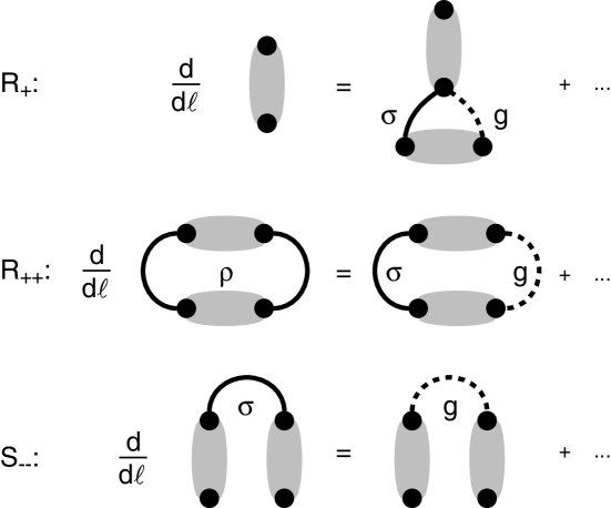
FIG. 1.: Diagrammatic representation of the flow equations (V). Black points stand for fields $\phi^{\alpha}({\bf x})$. A shaded oval “vertex” connection between two points means that they are evaluated at the same position (however, in general their replica index is different) and that their difference is the argument of a function. A line connecting two fields represents a kernel function (a broken line represents $g$; full lines represent $\sigma$ or $\rho$). Fields connected by a line are confined to the same replica. Scaling terms and topologically equivalent diagrams are not included in this illustration. At the fixed point an oval connection is related to a derivative $R_{+}^{(1)}$. The number of lines leaving a vertex equals the order of the derivative. The point order is given by the number of vertices. The replica order is given by the number of disconnected groups of fields. Diagrams in which a $g$ line would connect points that are already connected via other lines do not contribute to the flow equations since they are of higher order in temperature. If both fields of a vertex are linked through lines and an odd number of lines leaves the vertex then the diagram vanishes for symmetry reasons.

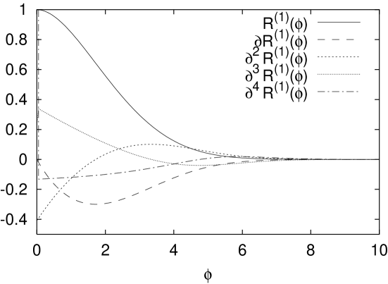
FIG. 2.: Illustration of the fixed-point function $R^{(1)}(\phi)$ and its first four derivatives. Note that $\partial^{3}R^{(1)}(0^{+})>0$. The singular contribution to $\partial^{4}R^{(1)}(\phi)$ is represented by the vertical part of the line near $\phi=0$.

REFERENCES

- [1] S. Lemerle, J. Ferre, C. Chappert, V. Mathet, T. Giamarchi, and P. Le Doussal, Phys. Rev. Lett. 80, 849 (1998).
- [2] T. Salditt, T. H. Metzger, J. Peisl, B. Reinker, M. Moske, and K. Samwer, Europhys. Lett. 32, 331 (1995).
- [3] D. S. Fisher, Phys. Rev. Lett. 56, 1964 (1986).
- [4] F. J. Wegner and A. Houghton, Phys. Rev. A 8, 401 (1973).
- [5] L. Balents and D. S. Fisher, Phys. Rev. B 48, 5949 (1993).
- [6] T. Giamarchi and P. Le Doussal, Phys. Rev. Lett. 72, 1530 (1994).
- [7] T. Emig, S. Bogner, and T. Nattermann, Phys. Rev. Lett. 83, 400 (1999).
- [8] P. Nozières and F. Gallet, J. Physique (Paris) 48, 353 (1987).
- [9] T. S. Chang, D. D. Vvedensky, and J. F. Nicoll, Phys. Rep. 217, 279 (1992).
- [10] J. Berges, N. Tetradis, and C. Wetterich, 2000, preprint arXiv:hep-ph/0005122.
- [11] K. G. Wilson and J. Kogut, Phys. Rep. 12, 75 (1974).
- [12] J. Polchinski, Nucl. Phys. B 231, 269 (1984).
- [13] G. R. Golner and E. K. Riedel, Phys. Rev. Lett. 34, 171 (1975).
- [14] P. Shukla and M. S. Green, Phys. Rev. Lett. 34, 436 (1975).
- [15] J. Rudnick, Phys. Rev. Lett. 34, 438 (1975).
- [16] G. Grinstein and S. K. Ma, Phys. Rev. Lett. 49, 685 (1982).
- [17] S. F. Edwards and P. W. Anderson, J. Phys. F 5, 965 (1975).
- [18] A. I. Larkin, Sov. Phys. JETP 31, 784 (1970).
- [19] K. B. Efetov and A. I. Larkin, Sov. Phys. JETP 45, 1236 (1977).
- [20] Y. Imry and S. K. Ma, Phys. Rev. Lett. 35, 1399 (1975).
- [21] M. Kardar, J. Appl. Phys. 61, 3601 (1987).
- [22] T. Nattermann, Europhys. Lett. 4, 1241 (1987).
- [23] F. Wegner, in Phase Transitions and Critical Phenomena, edited by C. Domb and M. S. Green (Academic, London, 1976).
- [24] At first sight it may not be obvious that the first term in Eq. (24) accounts for the rescaling of lengths. This functional form for rescaling was used previously, e.g., in Ref. [23], Eq. (3.158).
- [25] J. Zinn-Justin, Quantum field theory and critical phenomena (Clarendon Press, Oxford, 1993).
- [26] U. Schulz, J. Villain, E. Brézin, and H. Orland, J. Stat. Phys. 51, 1 (1988).
- [27] D. A. Huse, C. L. Henley, and D. S. Fisher, Phys. Rev. Lett. 55, 2924 (1985).
- [28] A. A. Middleton, Phys. Rev. B 52, R3337 (1995).
- [29] Y. Dinçer, Zur Universalität der Struktur elastischer Mannigfaltigkeiten in Unordnung, diploma Thesis, Universität zu Köln (1999).
- [30] S. Scheidl, unpublished (2000).
- [31] D. S. Fisher and D. A. Huse, Phys. Rev. B 43, 10728 (1991).
- [32] T. Hwa and D. S. Fisher, Phys. Rev. B 49, 3136 (1994).