Inherent structures and non-equilibrium dynamics of 1D constrained kinetic models: a comparison study

Abstract

We discuss the relevance of the Stillinger and Weber approach to the glass transition investigating the non-equilibrium behavior of models with non-trivial dynamics, but with simple equilibrium properties. We consider a family of 1D constrained kinetic models, which interpolates between the asymmetric chain introduced by Jäckle and Eisinger [Z. Phys. B84, 115 (1991)] and the symmetric chain introduced by Fredrickson and Andersen [Phys. Rev. Lett 53, 1244 (1984)], and the 1D version of the Backgammon model [Phys. Rev. Lett. 75, 1190 (1995)]. We show that the configurational entropy obtained from the inherent structures is the same for all models irrespective of their different microscopic dynamics. We present a detailed study of the coarsening behavior of these models, including the relation between fluctuations and response. Our results suggest that any approach to the glass transition inspired by mean-field ideas and resting on the definition of a configurational entropy must rely on the absence of any growing characteristic coarsening pattern.

I Introduction

There is an old debate concerning the correct description of dynamics in the glassy state [1]. According to the general wisdom, undercooled liquids are in a locally equilibrated metastable phase, but fall completely out of equilibrium when the relaxation time exceeds the observation time. In this situation the glass ages and slowly relaxes towards equilibrium. While it is widely accepted that the glass transition observed in laboratory is a purely kinetic phenomenon, it is still not clear whether a true (or what kind of) ergodicity breaking underlies the glassy behavior and whether the properties associated to a possible equilibrium transition manifest themselves on the experimentally accessible time scales. A particularly interesting problem concerns the precise mechanism leading to a slow relaxation and its relation with the ground states structure of the system.

A possible description of the non-equilibrium regime is in terms of coarsening. The coarsening process is described by a length scale which grows in time driving the system towards equilibrium. The most typical scenario for a coarsening dynamics is found in a ferromagnet quenched down to a temperature below its critical temperature $T_{c}$. After quenching, domains of positive and negative magnetization grow with time. The system acquires a macroscopic magnetization only when the typical domain size becomes of the order of the system size, leading to a nucleation process which involves overturning of large domains in favor of the dominant phase. Although it cannot be excluded that some type of coarsening behavior similar to that found in ferromagnets takes place in real glasses, there is no strong evidence, up to now, that any type of coarsening process occurs in the relaxation of an undercooled liquid.

Another possible description for the observed non-equilibrium behavior calls for activated dynamics. The activated dynamics scenario is rather different from coarsening. No typical growing length scales are now present. The system approaches a disordered state, which has no correlation with the crystal state, via thermally activated jumps among different configurations corresponding to structural rearrangements of spatially localized regions. In this scenario, the ordered crystal state has no special relevance. It occurs when fluctuations nucleate a crystalline droplet of size bigger than a given critical size, strongly dependent on external parameters such as temperature. Consequently crystallization can be completely inhibited by going to low enough temperatures. It is generally assumed that crystallization plays a role only for time scales much larger than those relevant for the relaxation of thermodynamic quantities in the undercooled phase (such as the enthalpy or specific heat). Indeed a glass transition also emerges for purely disordered systems where a crystal state does not exist [2, 3]. This does not exclude the presence of heterogeneities in the glassy phase, whose role and influence on the dynamics still needs to be understood [4, 5].

Despite the enormous effort devoted to this subject it is still not clear how these two scenarios combine together into a final description of the glassy state. Moreover, if coarsening is the driving process for the relaxation of undercooled liquids, due to the completely unknown microscopic structure of the glass state (on which the system should asymptotically relax) it is unclear what should be experimentally measured in order to identify the growing domains. A similar problem is encountered in spin glasses [6]. Since a disordered state has not a periodic structure, a priori one does not know how to observe domains and the question of the nature of the domains in spin glasses is still unresolved [7]. However, for spin glasses such freezing of temporal spin correlations leads to a divergence of the spin-glass susceptibility. Despite some experimental [8] and simulation results [5, 9], strong evidence for such a divergence is not found in structural glasses. The greatest difficulty in elucidating this issue is that a general non-equilibrium theory to deal with this class of systems is still missing and approximations to this problem remain partial. They usually work either in a limited range of time scales or in a limited range of temperatures (for instance, mode-coupling theory [10]).

During the eighties a novel approach to the glass transition was proposed by Stillinger and Weber [11]. This description of the undercooled liquid phase, inspired by the Adams-Gibbs-Di Marzio [12] theory, incorporates those features of the energy landscape relevant to the activated regime. The Stillinger-Weber approach is based on a decomposition of the configurational space into basins (also called inherent structures, hereafter referred to as IS) on the basis of the topology of the potential energy surface. This construction yields a definition of a configurational entropy in terms of dynamically accessible basins and it is close in spirit to the equilibrium configurational entropy or complexity of mean-field spin-glass models [13, 14].

In this paper we study the relevance of the IS analysis proposed by Stillinger and Weber for non-equilibrium dynamics using one-dimensional constrained kinetic models. Kinetically constrained models were first proposed by Fredrickson and Andersen [15] in the attempt to provide a simple microscopic mechanism for understanding the purely dynamical transition predicted by the mode-coupling theory. In these models the slowing down of the dynamics is obtained through the introduction of dynamical constraints, compatible with detailed balance and Boltzmann-Gibbs distribution. What makes highly peculiar the relaxational behavior of these models is the fact that the slowing down of dynamics is only due to kinetic constraints, which prevent certain transitions from occurring. For a review on early results on these models see Ref. [16].

We find that the non-equilibrium properties of this class of models cannot be described in terms of the Stillinger and Weber approach, in contrast to what is found in other models of structural glasses such as Lennard-Jones glasses [14, 17, 18, 19] or finite-size fully connected disordered spin glasses [20]. The main reason is that even though the dynamics is different, the configurational entropy derived from the Stillinger and Weber decomposition is the same for all models. While this conclusion is probably valid for all type of coarsening models, it is an open problem whether the precise mechanism for which the inherent structure entropy happens to coincide is more general and independent of coarsening behavior, i.e. it could also hold for higher dimensional constrained models with a different dynamics.

The paper is organized as follows. In Section II we introduce the family of one-dimensional models studied. In Section III we discuss the Stillinger and Weber approach and the configurational entropy for these models. In Section IV we analyze and compare the non-equilibrium dynamics for the different models, in particular we consider the coarsening phenomena and the fluctuations response relation. Finally in Section V we present conclusions and discussion. Some technical points are analyzed in two Appendices.

II The models

We consider two different classes of 1D constrained models: the constrained Ising chain and the Backgammon (BG) model. For the former we shall mainly consider the two extreme cases of the symmetrically constrained chain (SCIC) introduced by Fredrickson and Andersen [15] and the asymmetrically constrained Ising chain (ACIC) introduced by Jäckle and Eisinger [21]. The BG model [22] is not a purely constrained kinetic model since there are not local constraint on the microscopic dynamics. The constraint here follows from the requirement that the number of particles remains constant. This induces a global dynamical constraint which slows down the dynamics as temperature is lowered. The study of the BG model complement our investigation comparing its behavior with the locally constrained Ising chain models.

1 The constrained Ising chain

The Hamiltonian of the model is defined by

$$E=-\sum_{i=1}^{V}\sigma_{i},$$ (1)

where $\sigma_{i}$ are Ising-like variables, which take the values $0,1$, and the index $i$ runs over the sites of a D-dimensional lattice of volume $V=L^{D}$. The model corresponds to a paramagnet in a field. The dynamics is of the Glauber type where the spins are randomly updated according to the following rule

$${\cal W}(\sigma_{i}\to 1-\sigma_{i})=\left[1-\frac{1}{D}\left(\sum_{\mu=1,D}(a\sigma_{i+\mu}+b\sigma_{i-\mu})\right)\right]\,\times\,\min\bigl{[}1,\exp(-\beta\Delta E)\bigr{]},$$ (2)

with $a$ and $b=1-a$ positive real numbers. In this paper we consider the 1D case $D=1$ although the model is also interesting for larger dimensions. With exception of the configuration with all spins equal to $1$ it is known that the space of configurations is an irreducible Markov chain, so that ergodicity is guaranteed and detailed balance is fulfilled.

Depending on the values of $a$ we may have different cases. In particular for $a=b=\frac{1}{2}$ the model corresponds to the SCIC [15],

$${\cal W}(\sigma_{i}\to 1-\sigma_{i})=\frac{1}{2}(1-\sigma_{i+1}+\sigma_{i-1})\,\times\,\min\bigl{[}1,\exp(-\beta\Delta E)\bigr{]}$$ (3)

so that a spin can flip iff at least one of its neighbors is down.

If $a$ is equal to $0$ or $1$ then the model corresponds to the ACIC ($a=0$) [21],

$${\cal W}(\sigma_{i}\to 1-\sigma_{i})=\min\bigl{[}1,\exp(-\beta\Delta E)\bigr{]}\,\times\,\delta_{\sigma_{i-1},0}.$$ (4)

In this case a spin can flip iff its left neighbor is down, and the dynamics is more constrained than in the SCIC. For generic values of $a$ the flipping of the spins may take a different probability depending if the left or right spin is down.

The vast majority of works appeared in the literature focused on the previous two cases (3) and (4). In the present paper, for completeness and for the scope of our discussion, we shall discuss when possible the behavior for generic $a$.

The dynamics of these models cannot be solved exactly, even if several important results are known. (i) The correlation time diverges in the low temperature limit as $\tau\sim\exp(2\beta)$ for the SCIC model [23, 24] and as $\tau\sim\exp(\beta^{2}/\log(2))$ for the ACIC model [25, 26]. (ii) In the SCIC model the staggered correlation functions relax exponentially fast with time and one can define two characteristic time scales[27]: the first one $\tau=1/(1+\exp(-\beta))$ non-activated, and the second one $\tau_{1}=\exp(\beta)$ activated. In particular the later defines the time scale before which no aging effects are seen in the correlation functions [27]. (iii) In the SCIC model the hierarchy of dynamical equations can be exactly closed for $T=0$ [27, 24]. In the Appendix A we show that this result, originally obtained for the SCIC model, can be easily extended to generic values of $a$.

2 The Backgammon (BG) model

The energy (Hamiltonian) of the Backgammon model is [22]

$$E=-\sum_{i=1}^{N}\delta_{n_{i},0},$$ (5)

where $n_{i}=0,1,\ldots,N$ counts the particles in each site (box) of a D-dimensional lattice of $N=L^{D}$ sites. The energy is given by the number of empty boxes. As before we consider the 1D case, where $D=1$. The dynamics is of the Kawasaki type where the particles are randomly moved from one box to another and the change is accepted with probability

$${\cal W}=\min\bigl{[}1,\exp(-\beta\Delta E)\bigr{]}.$$ (6)

Strictly speaking the BG model is not a constrained kinetic model since there are not local constraints on particles (or boxes). Nevertheless the conservation of particles number introduces a global constraint which makes the dynamics of the BG model glassy at low temperatures where a lot of particles accumulate in a small number of boxes and the further emptying of boxes becomes slower and slower as time goes on.

In the original definition the dynamics of this model was mean-field in the sense that particles could move from one box to any other box. This dynamics can be closed exactly [28] and many results have been obtained on its non-equilibrium behavior [29, 30]. Here we are interested in the equivalent one-dimensional case where boxes are located on a closed ring (a chain with periodic boundary conditions) and particles can only move from one box to its left or right neighboring boxes. In this case the dynamics at low temperatures is driven by the coarsening of clusters of empty boxes similarly to that of spin-1 domains in the kinetically constrained Ising chain. Here, however, in addition to temperature-activated processes induced by energy jumps, the system has entropic barriers which contribute in a non trivial way to the coarsening dynamics. In the original model [22] with mean-field dynamics coarsening was absent and the entropic barriers were the only responsible for glassy dynamics leading in that case to an activated behavior.

All these models share the common fact that, despite their dynamics, the thermodynamics is trivial and there are no equilibrium spatial correlations at any temperature. In particular, they do not show any finite-temperature phase transition. Therefore the non-trivial behavior follows only from the dynamics, which, dynamically constrained in the first case and ruled by entropic barriers in the second case, turns out to be glassy.

In the next Sections we present a detailed investigation of the non-equilibrium dynamics of these models and discuss how their dynamics cannot be efficiently described in terms of an IS based configurational entropy approach.

III The Stillinger and Weber entropy

A The Stillinger and Weber approach

An interesting approach to investigate activated behavior in glasses was suggested in the eighties by Stillinger and Weber [11]. This is based on the (natural) decomposition of the motion near the glass transition into intra-basin motion (within a valley) and inter-basin motion (jumps between valleys). In a “cage” picture the first motion corresponds to the motion of particles within a cage, while the second one to the creation or destruction of cages. This approach implements in a practical way the old idea that in the undercooled liquid a strong separation of timescales of the two motions occurs near the glass transition. The approach bears some resemblance to the Edwards packing entropy in the context of granular systems [31, 32].

Within the Stillinger and Weber (SW) approach each configuration of the system is mapped into a local minimum of the energy through a local potential energy minimization which start from the given configuration. The local minimum was called inherent structure (IS), while the set of configurations flowing into it defines the basin of attraction or valley of the IS. Following SW one then constructs a IS-based thermodynamics decomposing the partition function sum into a sum over IS with the same energy [11]

$${\cal Z}(T)\simeq\sum_{e}P_{IS}(e,T),$$ (7)

with

$$P_{IS}(e,T)=\exp\,N\,\left[-\beta e+s_{c}(e)-\beta f(\beta,e)\right],$$ (8)

where $s_{c}(e)$, defined as the configurational entropy, yields the number of different IS with energy $e$: $\Omega(e)=\exp(Ns_{c}(e))$. The term $f(\beta,e)$ accounts for the free energy of the IS-basin of energy $e$, i.e., the partition sum restricted to the basin of attraction of IS with energy $e$. In each IS-basin the energy has been shifted, so that the IS has zero energy, and $f$ accounts only for energy differences. In general $f(\beta,e)$ may have a non-trivial dependence on the energy if the IS-basin of IS with different energy are quite different. When the temperature is such that only the states near the bottom of the IS-basin do contribute then it is reasonable to expect that $f(\beta,e)$ is roughly independent of $e$ [18, 19, 20]. Another case where the dependence of $f(\beta,e)$ on $e$ is expected to be negligible is when the IS-basins are narrow and contain few configurations. This approximation works very well for REM-like models [33, 20]. When the $e$-dependence of $f$ can be neglected the configurational entropy $s_{c}(e)$ can be obtained directly from (8).

As long as the configurations counted on the r.h.s. of eq. (7) are the most relevant for the thermodynamics at temperature $T$ the above construction is totally legitimate as far as thermodynamics is concerned. It is only a different way of summing the partition function. Nevertheless the $s_{c}(e)$ obtained with the SW decomposition is in some sense a dynamical quantity since the projection between configurations and IS basins can be seen as the zero-temperature dynamics of the model. For this reason we will refer to it as Stillinger-Weber configurational entropy to distinguish it from other possible definitions of the configurational entropy taken from mean-field concepts [14, 17]. This poses the question, first raised by Monasson and Biroli[34], on the relevance of $s_{c}(e)$ and IS in general for dynamics.

It is clear that once the energy and the rules of the dynamics are given the IS can always be defined. For example for spin-glass models with quenched disordered variables taken from a continuous distribution, the dynamics usually consists of Monte Carlo updates (for instance, single spin-flips). The IS are then identified as the final configurations reached after a sequence of Monte Carlo moves where the spin which yields the largest decrease of energy is identified and flipped. Consequently, IS are stable against single spin-flips but not for higher-number of spin flips. Biroli and Monasson [34] conclude then that IS are ill-defined because $s_{c}(e)$ depends on the number of spin-flips, which make the configuration stable (at least, for not-fully connected models). We disagree with this conclusions because, as noted above, the IS and the SW entropy are intimately related to dynamics, and therefore it is not a surprise that changing the dynamics the IS and the SW entropy in general change. What, in our opinion, is ill-defined is to speak of IS without specifying the dynamics.

Nevertheless the question posed by Biroli and Monasson is far from being trivial. Indeed despite the fact that the IS and the SW are dynamical quantities it is far from obvious that they contain all (or almost all) relevant informations on the dynamics on long time scales. This is a well known problem in the theory of dynamical systems. The SW decomposition can be seen as a mapping of the true dynamics at a given temperature onto a symbolic dynamics given by the dynamics of the IS. The obtained symbolic dynamics gives a good description of the original one only if the mapping defines what is called a “generating partition”, see e.g. [35]. In general for a generic dynamics it is not at all trivial to demonstrate that such a partition exists, and even if it does exist, how to find it. We can then recast the question posed by Biroli and Monasson in the following way: does the SW decomposition lead to a generating partition, or at least to a good approximation of it, for the long time dynamics of glasses near the glass transition?

In general we can answer to this question only a posteriori. We define a possible partition and then check if this reproduces the desired features of the dynamics. However we can try to find under which conditions the answer could be affirmative. Usually to find a generating partition, or a good approximation of it, a good starting point is by looking at the “physical” properties of the dynamics. The SW mapping replaces each configuration in a IS-basin with the IS itself. Therefore it is clear that this mapping will be a good mapping if the systems spends a lot of time inside the basin. Under this assumption the dynamics on time scales larger than the typical residence time inside a IS-basin should be quite well described by the IS dynamics. This scenario is typical of a many valley dynamics with activated dynamics. It is also clear from the above discussion that if the IS mapping is a good mapping it does not matter which configuration inside the IS-basin is used to represent the IS-basin. It may be the IS itself or any other configuration in the basin. In a recent study of finite-size mean field spin-glass models, which share the properties of structural glasses, this independence has been indeed observed [20].

On the contrary for dynamical processes described by a coarsening process this description should in general fail because dynamics proceeds through geometrically correlated configurations. Barrat, Burioni and Mezard have shown [36] that the difference between the two scenarios has a simple manifestation in how dynamical trajectories departing from the same configurations separate in the phase space. Consider a system described by a vector $\vec{X}(t)$ in configuration space. At time $t_{w}$ the system is cloned into a new system described by the vector $\vec{Y}(t)$. The two copies are let evolve with different realizations of thermal noise and the overlap $Q_{t_{w}}(t)=\vec{X}(t_{w}+t)\cdot\vec{Y}(t_{w}+t)$ is recorded as a function of time $t$. For coarsening-like systems (called type I systems in [36]) the overlap converges to a finite value $Q_{\infty}=\lim_{t\to\infty}Q_{t_{w}}(t)$ for any value of $t_{w}$ while for glassy systems with structural glasses behavior (called type II systems in [36]) that limit gives, for all possible values of $t_{w}$, the lowest possible value of $\vec{X}(t_{w}+t)\cdot\vec{Y}(t_{w}+t)$. Since in general it is possible to define IS also for coarsening systems, this is an indication that in these systems the non-equilibrium dynamics goes through configurations that are unrelated with the IS. Most probably the relevant configurations for coarsening are those on the border among IS-basins, i.e., those configurations which are not mapped into any IS. In this case the IS and the SW configurational entropy can still be defined but are obviously of little use for understanding non-equilibrium dynamics, as shown by the results reported in the following Sections.

Before addressing the SW approach to non-equilibrium dynamics of constrained kinetic models we note that the definition of the SW configurational entropy may not be completely free of ambiguities, especially for systems with discrete states. Indeed the SW mapping assumes that once the energy and the dynamics are given then the mapping between configurations and IS is uniquely defined. This means that regardless of when a given configuration appears in the dynamical evolution it will always be mapped to the same IS. In most of the recent papers on this subject [18, 19, 20] this was the case, but for discrete models with discretized values for the energies, as the ones studied here, there may be problems because there could be many directions in phase space where the energy decreases by the same amount. In this case some “decision” must be taken, e.g., one could employ a random choice among the possible directions. The IS and the corresponding SW configurational entropy can still be defined, but now they depend on the chosen strategy for dealing with equivalent directions. It can be shown [37] that this leads to a temperature dependence of $s_{c}$, so that the form of $s_{c}$ depends on $T$. Only when some additional requirements are fulfilled the temperature dependence disappears. For example when all possible strategies lead to the same sampling rate for the IS relevant for the dynamics. We anticipate that this requirement is not fulfilled by the constrained kinetic models nor by the BG model studied here, and in some cases we find different curves for $s_{c}$ for different temperatures. Nevertheless the violation is not too strong since we basically find only two different curves depending on the temperature range. This reflects the trivial fact that the constraint is more or less effective depending on the temperature because more we lower the temperature more the system orders. Another interesting feature of these models is that, despite the fact that the properties of these dynamical models are rather different, all of them have the same SW configurational entropy $s_{c}$. This casts doubts on the relevance of the IS analysis for the non-equilibrium dynamics of these models.

B The kinetically constrained Ising chain

These models are defined by eqs. (1) and (2). To compute $s_{c}(e)$ we thermalize the system at a finite temperature $T$. This can be achieved either by running the dynamics for a sufficient long time or by starting from equilibrium configurations whose distribution is given by

$$P_{eq}(\sigma_{i})=\frac{\exp(\beta\sigma_{i})}{1+\exp(\beta)}.$$ (9)

For each thermalized configuration the corresponding IS is computed via the minimization process given by the zero-temperature dynamics. Repeating the procedure for several initial configurations the IS probability distribution (8) can be evaluated.

Each IS is a fix-point of the dynamics, and therefore we can estimate $s_{c}$ from the number of fix-points. This is easily evaluated denoting with $A$ the one-bit sequence $1$ and $B$ the two-bits sequence $01$ since all fix-points are given by all possible arbitrary sequences of $A$’s and $B$’s (for instance, the sequence $ABBBAABB$). If $N_{A},N_{B}$ stand for the number of $A$’s and $B$’s in the sequence, with $N_{A}+2N_{B}=N$, where $N$ is the length of the chain, then

$$N_{fix}=\frac{(N_{A}+N_{B})!}{N_{A}!N_{B}!}.$$ (10)

From this expression, and noting that $e=-(N_{A}+N_{B})/N$, we have

$$s_{c}(e)=\frac{\log(N_{fix})}{N}=-e\log(-e)-(1+e)\log(1+e)+(1+2e)\log(-1-2e).$$ (11)

The above formula assumes that all IS are counted with an equal a priori probability. This is what is called the method of unbiased guess in information theory [35]. Therefore the above expression is valid iff the dynamics samples (almost) all fix-points with equal probability, where with “almost” we mean the fix-points relevant for equilibrium dynamics at temperature $T$.

A better estimate of $s_{c}$ comes from the analysis of the zero-temperature dynamics. As shown in Appendix A the zero-temperature dynamics can be solved exactly for any value of $a$, and from this $P_{IS}(e,T)$ can be evaluated:

$$P_{IS}(e,T)=\frac{1}{\sqrt{2\pi\langle C_{0}^{2}(\infty)\rangle_{c}}}\exp\Bigl{(}-\frac{(e-\langle e_{IS}\rangle)^{2}}{2\langle C_{0}^{2}(\infty)\rangle_{c}}\Bigr{)}.$$ (12)

The details of the calculation are reported in the Appendices together with the expressions of $\langle C_{0}^{2}(\infty)\rangle_{c}$ and $\langle e_{IS}\rangle$, eqs. (62) and (59). Note that this result, as well as eq. (11), does not depend on the value of $a$ implying that all models, and in particular the SCIC and ACIC, have the same $P_{IS}(e,T)$ and hence the same SW configurational entropy.

In Fig. 1 we compare the numerically evaluated $P_{IS}(e,T)$ for the SCIC model with $N=64$ and different temperatures with the analytical prediction eq.(12). The agreement is quite good at low temperature but decreases with increasing temperatures where the variance of the Gaussian is slightly larger than in simulations.

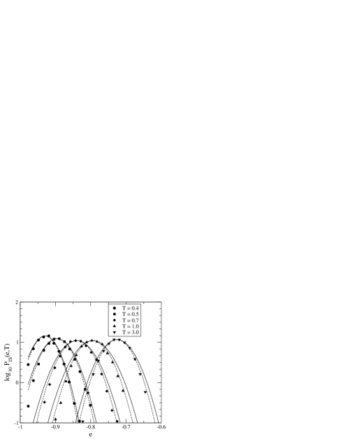
FIG. 1.: Probability histograms in the SCIC model with 64 spins at different temperatures compared with the analytical prediction (12) (full curve) and a fit to a Gaussian (dashed curve).

In Fig. 2 we report the average IS energy as a function of $T$ and compare it with the prediction from the analytical calculation of Appendix B. There are two possible ways to compute $e(T)$: the first is from eq. (59), the second rests on integrating the variance

$$e(T)=\int_{0}^{T}\frac{\langle C_{0}^{2}(\infty)\rangle_{c}}{T^{2}}\,dT,$$ (13)

where $\langle C_{0}^{2}(\infty)\rangle_{c}$ is given by (62). We also report the result from the fix-point approximation (11). Fig. 2 clearly shows that the different approximations depart each other at a temperature $T\simeq 0.6$. Above this temperature the energy dependence of the IS free energy $f$ in eq. (8) cannot be neglected anymore, showing that the fix-point approximation which neglects thermal fluctuations inside the IS-basins is inappropriate. On the other hand the direct calculation from the zero-temperature dynamics turns out to be very good.

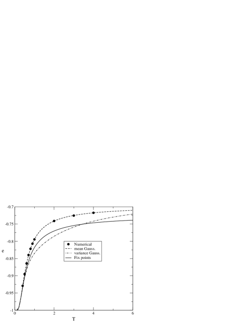
FIG. 2.: IS energies as function of temperature obtained integrating (11), using (59) and the variance of the IS-energy distribution given by (13).

Finally we consider $s_{c}$. In Fig. (3) we show the results obtained for the SCIC model with $N=64$ and different temperatures. The SW configurational entropy $s_{c}$ is obtained from the numerical $P_{IS}(T,e)$ as [19, 20]:

$$s_{c}(e)=\beta e+\log(P_{IS}(T,e)/N)+{\rm const}.$$ (14)

For each temperature the constant has been fixed by collapsing different data onto the single curve. As a comparison we also show the theoretical predictions from equations (11) and [See Appendix B]

$$s_{c}(e)=\int_{0}^{T}\frac{d\langle e_{IS}\rangle}{dT}\frac{dT}{T}.$$ (15)

As shown in the Appendix B, both coincide asymptotically close to the ground state energy $e=-1$. The collapse is excellent showing that the approximation (11) and the low-temperature behavior (15) asymptotically coincide in the limit $T\to 0$. We note that there is a range of energies where data from $T\leq 0.6$ collapse on one curve while data for higher temperature collapse on a different curve. As discussed above, this residual temperature dependence follows from the presence of many equivalent directions for energy minimization.

We have checked that $P_{IS}(T,e)$ is independent of $a$ by repeating the analysis for the ACIC model and for different values of $a$. In all cases we always find the same results.

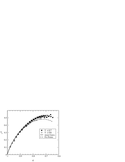
FIG. 3.: SW configurational entropy in the SCIC for $N=64$ spins at different temperatures compared with the analytical prediction (15) (upper curve) and the fix-point estimate (11) (lower curve).

C The BG model

In this case we cannot exactly solve the zero-temperature dynamics of the model and compute the SW configurational entropy. Nevertheless, we can approximate $s_{c}(e)$ of the BG model by counting the number of ways in which two or more particles can be distributed in a set of $N$ occupied boxes separated by empty boxes. This yields two contributions: the first comes from all possible ways of distributing the $M$ occupied boxes in a chain of $N$ boxes, with the additional condition that each occupied box is surrounded by an empty box. This is again given by eq. (10) assuming that $\sigma=1$ for occupied boxes and $\sigma=0$ for empty ones. The energy (5) is given by $E=-(N-M)$ and therefore this contribution reads,

$$s_{c}^{first}(e)=-(1+e)\log(1+e)-e\log(-e)+(1+2e)\log(-1-2e).$$ (16)

The second contribution follows from considering all different ways of distributing the $N$ particles among the $M$ occupied boxes with the constraint that each occupied box contains at least two particles:

$$N_{fix}^{second}=\sum_{\prod_{r=1}^{N}n_{r}\geq 2}\frac{1}{\prod_{r}n_{r}!}\delta(\sum_{r=1}^{N}{n_{r}}-N).$$ (17)

where the $n_{r}!$ terms arise from the distinguishability of particles. Introducing the integral representation for the delta function,

$$\delta(x)=\frac{1}{2\pi}\int_{-\infty}^{\infty}\exp(i\lambda x)\,d\lambda,$$ (18)

we find an expression for (17) in terms of the fugacity $y$. In the $N\to\infty$ limit this can be evaluated by the saddle point method yielding

$$s_{c}^{second}(e)=\frac{\log(N_{fix}^{second})}{N}=-\log(y)+(1+e)\log(\exp(y)-y-1),$$ (19)

where $y$ satisfies the saddle-point condition,

$$e=-1+\frac{\exp(y)-1-y}{y(\exp(y)-1)}.$$ (20)

The full entropy is given by

$$s_{c}(e)=s_{c}^{first}(e)+s_{c}^{second}(e).$$ (21)

Note that for this model the configurational contribution may be negative because particles are distinguishable.

We have computed $s_{c}(e)$ numerically following a procedure similar to that described for the constrained kinetic models. The results are shown in Fig. 4 for two different sizes $N=100,500$ and temperatures ranging from $T=0.1$ up to $T=1$. Similarly to what found for the constrained kinetic models, the data nicely collapse onto a single curve although it does not exactly coincide with the number of fix points. In this model the presence of different equivalent directions to decrease the energy does not influence $s_{c}$. This is most probably due to the global character of the constraint.

Comparing Figs. 3 and 4 we see that the agreement now is worse. We attribute this to the presence of entropic barriers which follows from all possible arrangements of particles inside the boxes. All arrangements leave the energy unchanged, but their number strongly depends on the number of empty boxes, leading to a stronger energy dependence of the IS free energy for this model. This effect was not present in the kinetically constrained Ising chain.

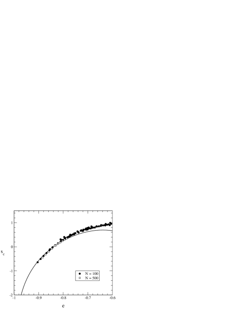
FIG. 4.: SW configurational entropy in the BG model for $N=100,500$ boxes at different temperatures $T=1.0,0.5,0.4,0.3,0.2,0.15,0.1$ compared with the fix-point estimate (21) (full line).

The conclusion that can be drawn from this Section is that for these models a description of the glassy behavior in terms of a complex energy landscape is not relevant. Even though the SW configurational entropy for the constrained Ising chain is a non trivial quantity, it does not distinguish the SCIC model from the ACIC model.

IV Analysis of coarsening behavior

In the previous Section we have seen that the IS approach yields identical results for models which are known to have a completely different dynamical behavior, namely the SCIC and ACIC models. The purpose of this Section is to evidentiate these difference making connection with results already known in the literature and studying new ones to gain some insight using the tools from disordered systems. Coarsening appears when domains of a given phase grow in time slowly enough for the system to be off-equilibrium [38]. In the simplest case, dynamics is characterized by a unique length scale associated with the typical size of the growing domains. All models discussed in this paper can be described in terms of coarsening in the sense that it is possible to define a length scale which identifies the distance from to equilibrium. For the kinetically constrained Ising chain this length is the typical size of the $+1$ domain while in the BG model it is the typical length of sequences of empty boxes.

In the simplest cases this length suffices to characterize the off-equilibrium behavior. For instance, for coarsening in (ordered or disordered) ferromagnets the off-equilibrium behavior is fully characterized in terms of a single length scale $L(t)$ in the sense that the two-times dependence of correlation and response functions directly enters through the value of this length scale. In the aging regime, where both times $t,s$ are large we have [38]

$$C_{ag}(t,s)\sim f\left(\frac{L(t)}{L(s)}\right),$$ (22)

$$R_{ag}(t,s)\sim\frac{1}{L(t)^{\alpha}}\,g\left(\frac{L(t)}{L(s)}\right),~{}~{}~{}~{}~{}~{}~{}~{}t>s,$$ (23)

with $\alpha\geq 1$ a positive exponent which depends on the model under consideration.

Correlations are easy to measure, while responses require the introduction of an external perturbation. This perturbation must couple with the variables of the system and must be small enough to ensure a linear response regime. A useful quantity is the integrated response function (hereafter denoted as IRF), which measures how much the system remembers the effects of a perturbation applied during a given interval of time [39],

$$\chi(t,s)=\int_{s}^{t}\,du\,R(t,u)$$ (24)

One of the salient features of coarsening phenomena [38, 40, 41] is that aging effects in the integrated response function asymptotically vanish when the lower time $s$ goes to infinity and the system does not have long-term memory. Suppose that the coarsening length $L(t)$ grows like $t^{1/z}$ with $z$ a dynamical exponent. Using eqs.(23) and (24) one finds that the aging part of the IRF behaves like,

$$\chi_{ag}(t,s)\sim s^{1-\frac{\alpha}{z}}\hat{\chi}(t/s)$$ (25)

which vanishes as $s\to\infty$ if $\alpha>z$.

An easy way to test these effects is by directly looking at fluctuation-dissipation plots (hereafter referred to as FDT) [42]. In equilibrium $R(t,u)=R(t-u)=\beta\frac{C(t-u)}{\partial u}$ which substituted into (24) yields,

$$\chi(t-s)=\beta[C(0)-C(t-s)]$$ (26)

and the plot of $T\chi(t,s)$ in terms of $C(t,s)$ is a straight line of slope $-1$.

In the off-equilibrium regime expression (26) can be generalized by defining the fluctuation-dissipation ratio [39]

$$X(t,s)=\frac{TR(t,s)}{\frac{\partial C(t,s)}{\partial s}}$$ (27)

which measures how far the system is from equilibrium. In equilibrium $X$ is equal to $1$. In the off-equilibrium asymptotic long-time regime, i.e. in the aging regime, where there is no time translational invariance both $X(t,s)$ and $\chi(t,s)$ are expected to be non-trivial functions of $C$. A quantitative estimate of $X$, can be obtained from the slope of the FDT plots:

$$X(C)=-\left[\frac{\partial\,T\chi(t,s)}{\partial C(t,s)}\right]_{C(t,s)=C}~{}~{}~{}~{}~{}.$$ (28)

For coarsening models the aging part of the IRF asymptotically vanishes and $\chi(t,s)$ is expected to saturate to a finite value, called the field-cooled value in the context of spin glasses, and stays constant while the correlation still decreases before saturating.

The simplest way to compute the IRF in the present class of models is to apply a perturbation which does not couple with the absorbing state, i.e., the ground state. We start from a random initial configuration and after a waiting time $s=t_{w}$ apply a random staggered field $h_{i}=\epsilon_{i}\,h_{0}(t)$, where $h_{0}(t)$ is the intensity of the field and $\epsilon_{i}=\pm 1$ are independent random quenched variables of zero mean. This method has the advantage that the perturbation term in the Hamiltonian does not directly couple to the coarsening length, and has been used by Barrat [43] to investigate coarsening in finite-dimensional Ising models.

The staggered magnetic field couples to the spin variables $\sigma_{i}$ in kinetically constrained models and to the equivalent variables $\sigma_{i}=\delta_{n_{i},0}$ in the BG model so that the perturbation in the Hamiltonian reads

$$\delta{\cal H}(t)=-\sum_{i=1}^{N}\,\epsilon_{i}\,h_{0}(t)\,\sigma_{i}~{}~{}~{}~{}~{}.$$ (29)

In the case of $h_{0}(t)=h_{0}\,\theta(t-t_{w})$ the integrated response function can be obtained measuring the random staggered magnetization after switching the field at time $s=t_{w}$ as,

$$\chi(t+t_{w},t_{w})=\frac{1}{N\,h_{0}}\sum_{i=1}^{N}\epsilon_{i}\,\sigma_{i}(t+t_{w}).$$ (30)

The original $0,1$ variables have some disadvantages, for example the correlation at equal time is not $1$ but depends on temperature. For this reason we find more convenient to work with the new variables $\nu=2\sigma-1$ which now take the values $1,-1$. We then consider the disconnected correlation,

$$C(t+t_{w},t_{w})=\frac{1}{N}\sum_{i=1}^{N}\nu_{i}(t_{w})\,\nu_{i}(t+t_{w})$$ (31)

and the staggered magnetization (30),

$$M_{stag}(t+t_{w},t_{w})=\frac{1}{N}\sum_{i=1}^{N}\epsilon_{i}\,\nu_{i}(t+t_{w})=2\,h_{0}\,\chi(t+t_{w},t_{w})$$ (32)

Now the equal times disconnected correlation function is equal to $1$ so that in the FDT plots, where the integrated response function is plotted versus the disconnected correlation function, all curves start from $C=1,M_{stag}\simeq 0$ for $t=t_{w}$. This makes easier to compare results from different values of $t_{w}$.

As discussed before in Section III a different way to distinguish coarsening dynamics from other more complex behaviors is to measure the overlap $Q(t)$ between two replicas which start from the same configuration at time $t_{w}$ and evolve with different realization of thermal noises. Here we consider the connected, normalized overlap function,

$$Q^{c}_{t_{w}}(t)=\frac{\frac{1}{N}\sum_{i=1}^{N}\sigma^{(1)}_{i}(t_{w}+t)\,\sigma^{(2)}_{i}(t_{w}+t)-\bigl{(}\frac{1}{N}\sum_{i=1}^{N}\sigma^{(1)}_{i}(t_{w}+t)\bigr{)}\bigl{(}\frac{1}{N}\sum_{i=1}^{N}\sigma^{(2)}_{i}(t_{w}+t)\bigr{)}}{\frac{1}{N}\sum_{i=1}^{N}\sigma^{(1)}_{i}(t_{w})-[\frac{1}{N}\sum_{i=1}^{N}\sigma^{(1)}_{i}(t_{w})]^{2}}$$ (33)

where $\sigma^{(1,2)}=0,1$ refer to the two replicas, and the connected, normalized, correlation

$$C_{c}(t+t_{w},t_{w})=\frac{\frac{1}{N}\sum_{i=1}^{N}\sigma^{(1)}_{i}(t_{w}+t)\,\sigma^{(1)}_{i}(t_{w})-\bigl{(}\frac{1}{N}\sum_{i=1}^{N}\sigma^{(1)}_{i}(t_{w}+t)\bigr{)}\bigl{(}\frac{1}{N}\sum_{i=1}^{N}\sigma^{(1)}_{i}(t_{w}+t)\bigr{)}}{\frac{1}{N}\sum_{i=1}^{N}\sigma^{(1)}_{i}(t_{w})-(\frac{1}{N}\sum_{i=1}^{N}\sigma^{(1)}_{i}(t_{w}))^{2}}$$ (34)

For type I systems $Q^{c}_{\infty}=\lim_{t\to\infty}Q^{c}_{t_{w}}(t)$ is finite. For type II systems this quantity converges in the $t\to\infty$ limit to the lowest accessible value, i.e. vanishes in the $t\to\infty$ limit. In equilibrium both (33) and (34) depend only on $t$ and the following relation is valid $Q^{c}_{t_{w}}(t)=C_{c}(2t)$. There are few numerical studies of $Q^{c}_{t_{w}}$ [36, 44]. For the models considered here the results from this analysis are, however, not so strong, the reason probably being that coarsening occurs in a disordered (i.e. paramagnetic) phase.

In the rest of this Section we investigate in detail coarsening length scales, correlations and responses for the non-equilibrium dynamics of models described in Section II. We note that although many results on timescales and coarsening length scales have been obtained in the literature [21, 23, 24, 25, 26, 27] almost nothing is known about the aging behavior in this type of models (partial results are shown in [27] for the SCIC).

A The SCIC model

It has been shown in [27] that the SCIC model has an activated timescale $\tau_{1}=\exp(\beta)$ characterized by an exponential decay of the staggered energy. For times smaller than $\tau_{1}$ there are no aging effects and only for times larger than $\tau_{1}$ non-equilibrium behavior with non-exponential relaxation and aging appear. From the decay of correlation functions a second activated timescale $\tau_{\rm corr}>\tau_{1}$ can be defined. To this end we have computed the equilibrium connected correlation function

$$C_{c}(t)=\frac{N\sum_{i=1}^{N}\sigma_{i}(0)\,\sigma_{i}(t)-\sum_{i=1}^{N}\sigma_{i}(0)\sum_{i=1}^{N}\sigma_{i}(t)}{N\sum_{i=1}^{N}\sigma_{i}(0)-(\sum_{i=1}^{N}\sigma_{i}(0))^{2}}$$ (35)

which is well described for all temperatures by the following functional form

$$C_{c}(t)=\left(\frac{1}{1+t/\tau_{1}}\right)^{\alpha}\exp(-at^{b}),$$ (36)

where $\alpha,a,b$ are three fit parameters and the activated timescale $\tau_{1}$ is introduced in the fitting function as an effective microscopic time. The results for $C_{c}(t)$ are shown in Fig. 5 for different temperatures, the lines are the best fits with form (36). This fits are in agreement with the asymptotic analytical predictions of Reiter and Jäckle [23] and Schulz and Trimper [24] but combined with the exponential timescale $\tau_{1}$ derived in [27]. In particular the exponent $\alpha$ is close to the value $1/2$ predicted in [23, 24] for very low temperatures.

FIG. 5.: Equilibrium connected correlation functions in the SCIC for temperatures ranging from $T=1.0$ down to $T=0.35$ fitted according to (36). Data have been averaged over 1000 thermalized initial conditions and $N=10^{5}$.

From the fit we can estimate $\tau_{\rm corr}$ as

$$\tau_{\rm corr}=\int_{0}^{\infty}C_{c}(t)\,dt~{}~{}~{}~{}~{}.$$ (37)

The results are shown in Fig. 6. The correlation time $\tau_{\rm corr}$ follows the Arrhenius type law $\tau_{\rm corr}\sim\exp(2\beta)$. This functional dependence of correlation time from temperature can be understood from the following phenomenological argument, based on defects annihilation in the SCIC. A defect separated by magnetized domains can disappear by anchoring defects along the chain. The typical time to anchor a defect is $\exp(\beta)$ while the length of the magnetized domains in equilibrium is of order $\exp(\beta)$. Because defects can be anchored starting form the right or from the left of a magnetized domain, the typical time to annihilate that domain is the sum of independent processes yielding $\tau_{\rm corr}\sim\exp(2\beta)$.

FIG. 6.: Correlation time in the SCIC computed using (37) and fitted with an Arrhenius behavior. The best fit gives $\tau_{\rm corr}=1.43\exp(1.93\beta)$

To investigate coarsening in the SCIC model we have measured the growth of the average domain length

$$d(t)=\frac{\sum_{l=1}^{N}\,l\,P_{t}(l)}{\sum_{l=1}^{N}\,P_{t}(l)}$$ (38)

where

$$P_{t}(l)=\sum_{i=1}^{N}\prod_{j=i}^{i+l-1}\sigma_{j}(t)\,[1-\sigma_{i+l}(t)][1-\sigma_{i-1}(t)]$$ (39)

is proportional to the probability of having a domain of spins $1$ of length $l$ at time $t$. For $t\to\infty$ $P_{t}$ converges towards the equilibrium length probability distribution

$$P_{eq}(l)=\frac{\exp(-\beta)}{\bigl{[}1+\exp(-\beta)\bigr{]}^{l}}$$ (40)

and the average length saturates to the equilibrium value

$$d_{\rm eq}=1+\exp(\beta)$$ (41)

FIG. 7.: Average domain length and magnetization in the SCIC model. The average length grows diffusively like $t^{1/2}$.

In Fig. 7 we present the average domain length as a function of time starting from a random initial condition. From the figure it follows that after $10^{6}$ MCS $d(t)$ is still well below the equilibrium value $d_{\rm eq}$ for temperatures as high as $T=0.2$ indicating that the systems has not yet equilibrated. In agreement with [23] a power law fit leads to $d(t)\sim t^{1/2}$ characteristic of diffusion [45]. In the lower part of Fig. 7 we show the relaxation of the energy as a function of time. These results combine the zero temperature exponential decay to the threshold energy[27, 24] $1/e$ with the slower decay towards equilibrium. Note that since the average domain length grows like $t^{1/2}$ while the equilibrium value for large $\beta$ is $d_{\rm eq}\sim\exp(\beta)$ we get for the correlation time $\tau_{\rm corr}\sim\exp(2\beta)$, as expected.

Further informations on the non-equilibrium behavior can be obtained from the analysis of the response to a staggered magnetic field as described in eqs. (28), (31) and (32). In Figs. 8 and 9 we show $M_{stag}(t+t_{w},t_{w})$ [see eq. (32)] and the correlation function $C(t+t_{w},t_{w})$ for temperature $T=0.3$ and $0.11$ and different waiting times $t_{w}$. The strength of the staggered field is $h_{0}=0.1$ while the system size is $N=10^{5}$. The horizontal lines indicate the equilibrium values

$$C^{eq}=\frac{1}{N}\sum_{i=1}^{N}\,\langle\nu_{i}\rangle^{2}=\left(\frac{1-\exp(-\beta)}{1+\exp(\beta)}\right)^{2}$$ (42)

and

$$M_{stag}^{eq}=\frac{1}{N}\sum_{i=1}^{N}\,\langle\nu_{i}\rangle=2h_{0}\frac{\beta\exp(\beta)}{[1+\exp(\beta)]^{2}}+O(h_{0}^{2})$$ (43)

FIG. 8.: Correlations and zero-field cooled magnetization in a staggered field in the SCIC model for $N=10^{5}$, $T=0.3$ and different waiting times $t_{w}=10,100,1000,10000$. The horizontal lines indicate the equilibrium values (42) and (43).

FIG. 9.: Correlations and zero-field cooled magnetization in a staggered field in the SCIC model for $N=10^{5}$, $T=0.11$ and different waiting times $t_{w}=10,100,1000,10000$. The horizontal lines indicate the equilibrium values (43).

The corresponding FDT plots are shown in Figs. 10 and 11, respectively.

Concerning Figs. 8, 9, 10 and 11 we note the following:

1. Aging in the correlation function appears for waiting times larger than the critical time $\tau_{1}=\exp{(\beta)}$ and survives even for times larger than the correlation time $\tau_{\rm corr}$. This can be seen from both correlation function and staggered magnetization. The equilibration time $\tau_{\rm eq}$ to reach equilibrium is larger than both the activated time $\tau_{1}$ and the correlation time $\tau_{\rm corr}$. If we define the equilibration time $\tau_{\rm eq}$ as the time needed for the average domain length to reach the equilibrium value, then plotting the data of Fig. 7 as function of $T\log(t/\tau_{0})$ we find that $\tau_{\rm corr}\sim\frac{\tau_{\rm eq}}{\tau_{1}}$, i.e. $\tau_{\rm eq}\sim\exp(3\beta)$.

2. The staggered magnetization has a hump, in correspondence of which the correlation function presents a broad minimum, as function of $t$. For $t_{w}\leq\tau_{1}$ the hump maximum takes the largest value and decreases with $t_{w}$ as soon as $t_{w}>\tau_{1}$ and eventually disappears for $t_{w}\to\infty$. This effect is a direct manifestation of the two critical timescales present in the SCIC model [27].

3. The existence of different activated relaxation times results in rather peculiar FDT plots, see Figs. 10 and 11. For $t_{w}<\tau_{1}$, Fig. 11, $C$, $\chi$ and $X$ do not show any dependence on $t_{w}$, nevertheless $X$ is a non-trivial function of $C$ corresponding to non-equilibrium behavior without aging. A similar shape is found for the one-dimensional Ising model at low temperatures [46]. For $t_{w}>\tau_{1}$, Fig. 10, there are aging effects and $X$ shows the typical two slope pattern. However, the existence of a second typical timescale results in a second downwards bending of the IRF and $X$ as function of $C$ has a three slope shape.

FIG. 10.: FDT plots in the SCIC for $N=10^{5}$, $T=0.3$ and different waiting times $t_{w}=10,100,1000,10000$. The straight line is the FDT relation (26)

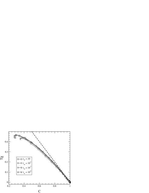
FIG. 11.: FDT plots in the SCIC for $N=10^{5}$, $T=0.11$ and different waiting times $t_{w}=10,100,1000,10000$. The straight line is the FDT relation (26)

We conclude the analysis of the SCIC model by discussing the results for the cloning experiment. In Fig. 12 we show the overlap $Q^{c}_{t_{w}}(t)$ [eq.(33)] as a function of the connected correlation $C_{c}(t+tw,t_{w})$ [eq.(34)] for temperature $T=0.11$. The results show that, for any finite $t_{w}$, $Q$ goes to zero quite rapidly. If one compares $Q^{c}_{t_{w}}(t)$ with $C_{c}(2t+t_{w},t_{w})$ for different values of $t_{w}$ one finds that both decrease exponentially fast with time and that $Q^{c}_{t_{w}}(t)$ is smaller but very close to $C_{c}(2t+t_{w},t_{w})$. This implies that the two trajectories depart form each other quite fast. The data in Fig. 12 collapse quite nicely onto the parabola $Q\simeq C^{2}$ in agreement with the exponential decay.

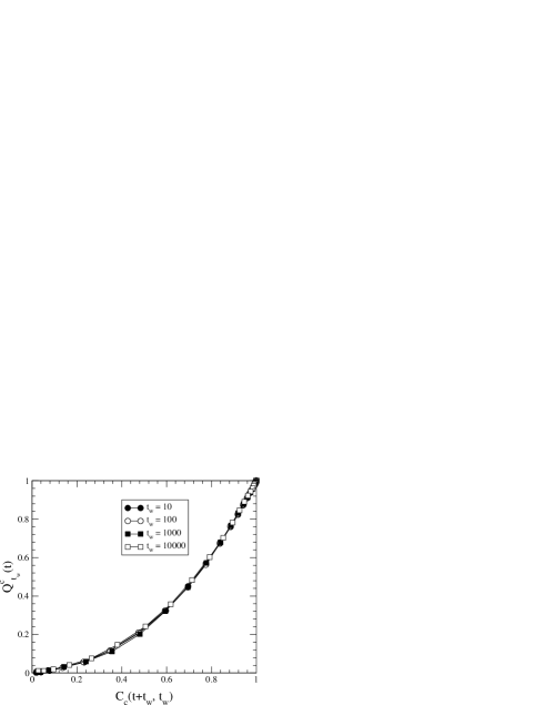
FIG. 12.: $Q^{c}_{t_{w}}(t)$ versus $C_{c}(t+t_{w},t_{w})$ in the SCIC at $T=0.11$

In conclusion the SCIC model is a coarsening model with three activated timescales $\tau_{1}=\exp(\beta)$, $\tau_{\rm corr}=\exp(2\beta)$ and $\tau_{\rm eq}=\exp(3\beta)$. In this scenario we do not expect the simple scaling form (22) in terms of a single length scale to be verified. Indeed, although a growing length scale can be identified a single length scale does not describe the whole time regime. This is clearly seen in Fig. 13 for $T=0.15$ where aging starts after $\tau_{1}\sim 1000$. The scaling form (22) constructed from data from Fig. 7 is shown in Fig. 14. The scaling is obviously rather poor. The behavior of this model is essentially diffusive as emerges from the behavior of the overlap $Q^{c}_{t_{w}}(t)$ similar to the behavior of a ferromagnet with non conserved order parameter, with the difference that the SCIC model has no phase transition and coarsening takes place in a disordered phase.

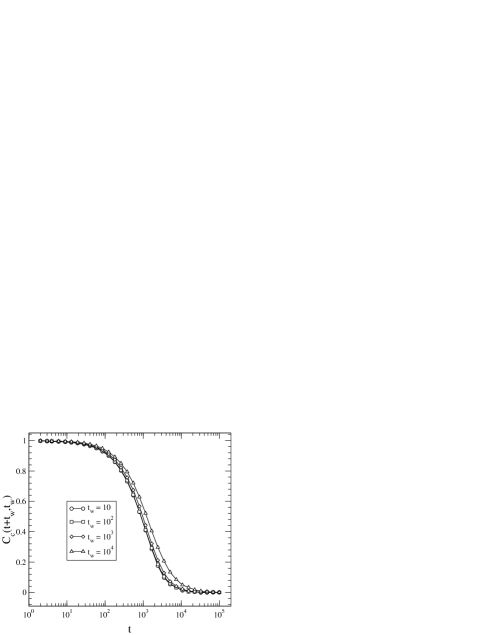
FIG. 13.: Connected correlations $C_{c}(t_{w},t_{w}+t)$ in the SCIC for $N=10^{5}$, $T=0.15$ and different waiting times $t_{w}=10,100,1000,10000$. Aging is present for times larger than $\tau_{1}=\exp(\beta)$

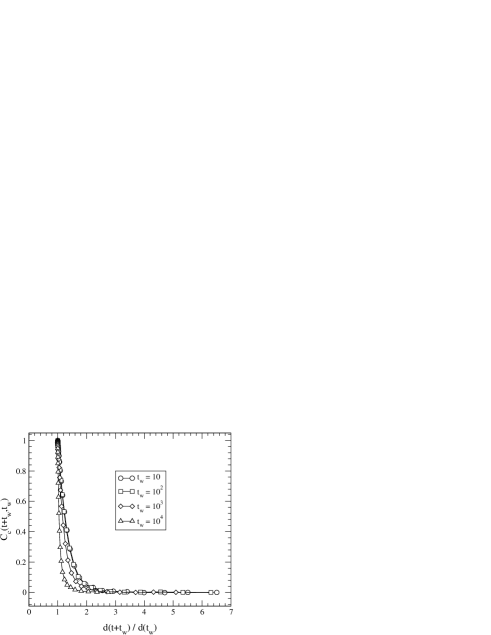
FIG. 14.: Connected correlations $C_{c}(t_{w},t_{w}+t)$ (34) in the SCIC for $N=10^{5}$, $T=0.15$ plotted versus $d(t+t_{w})/d(t_{w})$.

B The ACIC model

Coarsening in this model has been extensively studied by several authors, finding that the correlation time has a super-Arrhenius behavior and grows like $\exp(\beta^{2}/\log(2))$ [25, 26], much faster than the typical Arrhenius behavior $\sim\exp(2\beta)$ found for the SCIC model. In the SCIC model domains can always grow if they can annihilate defects by building intermediate defects to the right or to the left of that defect. In the ACIC model, on the contrary, defects can disappear only by anchoring intermediate defects in the middle of the domain from one side. This strongly enhances the correlation time. On the other hand, the absence of a critical time like $\tau_{1}$ and the coincidence of the correlation time with the equilibration time makes the dynamics of this model simpler than that of the SCIC model.

In Fig. 15 we show the average domain length defined by eq. (38) and the energy as a function of time when starting from a random initial configuration for different temperatures. The $T\log(t)$ scaling predicted by Sollich and Evans [26] is very well satisfied. Note the presence of plateaus in both the average domain length and the energy for the same range of time. These correspond to time intervals where domains coalesce and the global energy stays constant because the number of anchoring spins is much smaller than the length of the coalescing domains [26]. Since the average domain length grows like $\log(d)\sim\lambda T\log(t)$, i.e., $d\sim t^{\lambda T}$, and the equilibrium domain length is given by $d_{\rm eq}\sim\exp(\beta)$ for low temperature, a phenomenological argument yields for the correlation time $\tau_{\rm corr}\sim\exp(\beta^{2}/\lambda)$ with $\lambda=\log(2)$ in agreement with the expectations of Mauch and Jäckle [25].

FIG. 15.: Average domain length and magnetization in the ACIC at $T=0.15,0.20$. The average length grows like $t^{\lambda T}$.

Figures 16 and 17 show the non-equilibrium disconnected correlation function (31) and the staggered magnetization (32) from infinite temperature initial conditions as a function of time for two temperatures $T=0.2$ and $0.4$ and different values of $t_{w}$. The strength of the field is $h_{0}=0.1$. The dashed horizontal lines are the equilibrium values (42) and (43). The FDT plots are shown in Figs. 18 and 19.

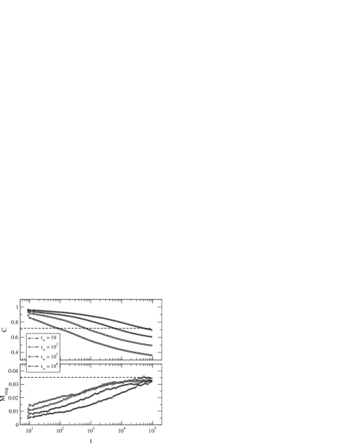
FIG. 16.: Correlations and zero-field cooled magnetization in a staggered field in the ACIC model for $N=10^{5}$, $T=0.4$ and different waiting times $t_{w}=10,100,1000,10000$. The horizontal line indicates the equilibrium value (43)

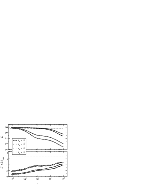
FIG. 17.: Correlations and zero-field cooled magnetization in a staggered field in the ACIC model for $N=10^{5}$, $T=0.2$ and different waiting times $t_{w}=10,100,1000,10000$. The horizontal line indicates the equilibrium value (43)

Looking at this set of figures we note the following points:

1. The staggered magnetization does not posses a hump, and the correlation functions a broad minimum, as in the SCIC model. Here, on the contrary, both are monotonic functions of time, a behavior commonly found in models where there is no critical time (like $\tau_{1}$ in the SCIC) associated with a microscopic fast process. On the timescale of $\tau_{\rm corr}$ both quantities relax to the equilibrium values. We note that $\tau_{\rm corr}\simeq 10^{4}$ for $T=0.4$ and $\tau_{\rm corr}\simeq 10^{15}$ for $T=0.2$.

2. A simple look at Figs. 16 and 17 reveals that aging is present for all timescales in both the correlation function and staggered magnetization. Aging in $M_{stag}$ is noticeable for all values of $t_{w}$ suggesting that aging in the IRF disappears rather slowly with $t_{w}$. Keeping in mind the coarsening nature of this model this suggests that $\alpha\simeq z$ in eq. (25).

3. From Figs. 16 and 17 it is difficult to verify the coarsening nature of the dynamics in this model. A simple check can be done with the help of the FDT plots shown in Figs. 18 and 19 for temperatures $T=0.4$ and $T=0.2$. Interestingly for waiting times comparable to the correlation time, so that the system is not far from equilibrium, the fluctuation-dissipation ratio $X$ rapidly converges to $1$, see Fig. 18. At low temperatures, Fig. 19, $t_{w}\ll\tau_{\rm corr}$ and the fluctuation-dissipation ratio is very small, $X\simeq 0.1$, and roughly independent of $t_{w}$, a scenario typical of coarsening models [43].

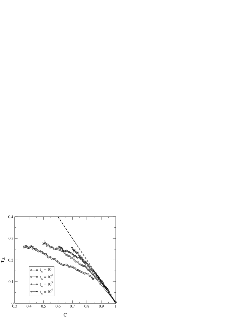
FIG. 18.: FDT plots in the ACIC for $N=10^{5}$, $T=0.4$ and different waiting times $t_{w}=10,100,1000,10000$. The straight line is the FDT relation (26)

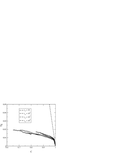
FIG. 19.: FDT plots in the ACIC for $N=10^{5}$, $T=0.2$ and different waiting times $t_{w}=10,100,1000,10000$. The straight line is the FDT relation (26)

In the ACIC model there is only one characteristic divergent timescale, namely $\tau_{\rm corr}$, and thus we expect that the scaling behavior (22) should be satisfied. Note that, contrarily to the SCIC, the average domain length $d(t)$ does not grow in time like a power law [see Ref. [26] and Fig. 15]. Consequently, in the aging regime the scaling will not be of the form $t/t_{w}$, see Fig. 20, but a more complicated function depending on shape of $d(t)$ [26], see Fig. 21 where $C_{c}(t_{w},t_{w}+t)$ is plotted as a function of $d(t_{w}+t)/d(t_{w})$. The scaling is quite good.

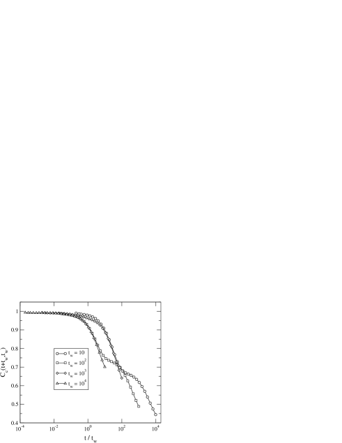
FIG. 20.: Connected correlations $C_{c}(t_{w},t_{w}+t)$ in the ACIC for $N=10^{5}$, $T=0.20$ and different values of $t_{w}$ plotted versus $t$

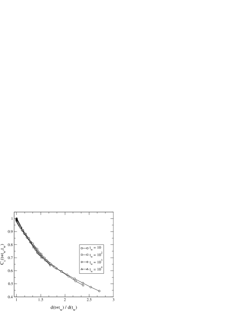
FIG. 21.: The same data of Fig. 20 plotted versus $d(t_{w}+t)/d(t_{w})$

We conclude our analysis of the ACIC model with the discussion of $Q^{c}_{t_{w}}(t)$ and $C_{c}(t+t_{w},t_{w})$ shown in Figs. 22 and 23. Again $Q^{c}_{t_{w}}(t)$ decays to zero for any $t_{w}$ but slower than in the SCIC model, see Fig. 12. If $Q^{c}_{t_{w}}(t)$ is compared with $C_{c}(2t+t_{w},t_{w})$ for different values of $t_{w}$ one finds that again $Q^{c}_{t_{w}}(t)$ is smaller, but very close to, $C_{c}(2t+t_{w},t_{w})$. However, contrarily to the SCIC case, now during the initial regime when $t_{w}$ is small both $Q^{c}_{t_{w}}(t)$ and $C_{c}(2t+t_{w},t_{w})$ show a plateau, more pronounced for $Q$, for times $t\simeq 10^{3}$. The time range between $t_{w}=10^{2}$ and $t_{w}=10^{3}$ corresponds [see Fig. 15] to the regime where $d(t)$ is growing very fast. This means that during this time interval domains grow, since $C$ slowly decays, but $Q$ remains almost constant because the two replicas follow the same narrow path in phase space. This effect is consequence of the way domains grow in this model where the anchoring of spins proceeds one by one in a given direction, different from the diffusive mechanism in the SCIC model. For $t_{w}$ larger than $10^{3}$ this effect would be observed at the next timescale, between $10^{5}$ and $10^{6}$, where new domains would have grown again [see Fig. 15]. Moreover this would also lead to a new plateau for $Q$ and $C$ for waiting times $t_{w}=10$ and $10^{2}$ for values of the correlation of order $0.3$ (which we have not reached in the simulations).

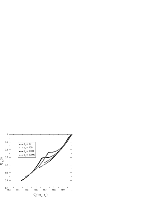
FIG. 22.: $Q^{c}_{t_{w}}(t)$ versus $C_{c}(t+t_{w},t_{w})$ in the ACIC at $T=0.2$

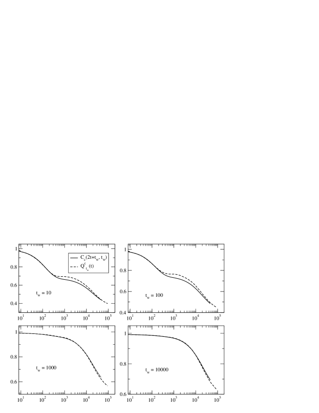
FIG. 23.: $Q^{c}_{t_{w}}(t)$ and $C_{c}(2t+t_{w},t_{w})$ in the ACIC at $T=0.2$

We can summarize the results of this subsection by saying that the non-equilibrium behavior of the ACIC model resembles coarsening in a simple ferromagnet although the growing length scale grows slower, like $t^{T\log(2)}$. The ansatz (22) for the scaling behavior is well verified and the FDT plots show some similarities with the physics of undercooled liquids although no connection between the slope of the FDT behavior and the SW configurational entropy is possible. Note that we obtain $X\simeq 0$ when temperature is lowered. Furthermore, the behavior of $Q^{c}_{t_{w}}(t)$ reveals that the relaxational dynamics proceeds by evolution in narrow channels in the time intervals where domains grow similar to what happens for type I models. On the contrary, it is not possible to establish the glassy scenario from the value of $\lim_{t\to\infty}Q^{c}_{t_{w}}(t)$ a quantity which we expect to work only for models with broken ergodicity.

C The BG model

In the 1D BG model, at difference with the kinetic constraint models discussed above, there are no dynamical constraints and coarsening follows from the slow growth of the number of empty boxes induced by entropic barriers. If we denote with $\sigma=0,1$ empty and occupied box, respectively, then we can consider the same quantities discussed for the kinetic constraint models, i.e., domain length probability distribution, average length, correlation and magnetization. All these quantities converge for large times to their equilibrium values derived from the equilibrium probability distribution [28],

$$P_{\rm eq}(n)=\frac{1}{N}\sum_{r=1}^{N}\langle\delta_{n_{r},n}\rangle=\frac{z^{n-1}\exp(\beta\delta_{n,0})}{n!\exp(z)}$$ (44)

which gives the probability that at equilibrium a box contains $n$ particles. Normalization of the distribution (44) corresponds to the conservation of the total number of particles, and reads

$$\exp(\beta)-1=(z-1)\exp(z).$$ (45)

By using $P_{\rm eq}$ the equilibrium values of correlations, response and domain length can be computed. For example the average domain length of empty boxes at equilibrium is given by,

$$d_{\rm eq}=\frac{1}{1-P_{\rm eq}(0)}$$ (46)

which diverges for $\beta\to\infty$ when all particles fill a single box. From the definition it follows that $P_{\rm eq}(0)$ is equal to minus the equilibrium energy (5) which, for small $T$, goes as $E/N=-1+T+O(T^{2})$. We then have $d_{\rm eq}\sim\beta$ for $\beta\to\infty$.

Similarly for the correlation function we have,

$$C^{\rm eq}=\frac{1}{N}\sum_{i=1}^{N}\,\langle\nu_{i}\rangle^{2}=[2P_{\rm eq}(0)-1]^{2}$$ (47)

where $\nu=2\sigma-1$.

To compute the staggered magnetization we have to use the equilibrium probability distribution with the extra term (29) added to the energy. A straightforward calculation leads to

$$M_{stag}^{\rm eq}=\frac{1}{N}\sum_{i=1}^{N}\,\langle\nu_{i}\rangle=\frac{e^{\beta}(1-e^{-z})\,\sinh(\beta h_{0})}{z\,(e^{z}-1+e^{\beta}\cosh(\beta h_{0}))}$$ (48)

where $z$ is now solution of

$$\frac{ze^{z}}{2}\,\left[\frac{1}{e^{z}-1+e^{\beta(1+h_{0})}}+\frac{1}{e^{z}-1+e^{\beta(1-h_{0})}}\right]=1.$$ (49)

Note that $M_{stag}^{\rm eq}$ is linear in $h_{0}$ for small values of $h_{0}$.

Analyzing in details the dynamics we can distinguish two different decay processes: the first one entropically activated and the second one energetically activated. When the system is quenched from high to low $T$ particles “evaporate” from some boxes and accumulate in others. After some time a situation is reached where boxes with more then one particle are separated by empty boxes and a very small number of single occupied boxes (defects). For $T=0$ these defects disappear and the energy does not relax to equilibrium. On the contrary for $T$ small but finite the number of these defects may be large enough, its number scaling as $TN$, to serve as nucleation paths between two nearby multiple occupied boxes which, by the usual entropic mechanism, eventually accumulate onto a single box. The timescale $\tau_{1}$ for this process is activated since defects must be created, but it is smaller than $\exp(\beta)$.

A second, energetically activated, process appears for defects to be anchored between multiple occupied boxes so that they coalesce in a single multiple occupied box. At low temperature and close to equilibrium the typical number of particles per occupied box is of order $\beta$ while the distance that particles must cover by diffusion from one box to a contiguous one is of order $d_{\rm eq}\sim\beta$. Combining these two behaviors we obtain for the equilibration time $\tau_{\rm eq}\sim\beta\exp(\beta)$.

The interplay between these two mechanisms can clearly be seen in Fig. 24 where we report growth of the average domain length, from an initial random configuration, and (minus) the average number of empty boxes (energy) as a function of time for different temperatures. The data are plotted as function of $T\log(t)$ so that the equilibration time, where the average length reaches the equilibrium value, is $T\log(\tau_{\rm eq})\simeq 1+\delta$ with $\delta=-T\log(T)$ leading to $\tau_{\rm eq}\simeq\beta\exp(\beta)$. This equilibration timescale $\tau_{\rm eq}$ is shorter than that of the kinetically constrained Ising chain but longer than the mean-field case $\tau_{\rm eq}\sim\frac{\exp(\beta)}{\beta^{2}}$ [29]. From the figure we also see that both the average domain length and the energy display a plateau at short times corresponding to the $T=0$ behavior. The departure from this initial plateau occurs for times shorter than the activated characteristic time $\exp(\beta)$ and is driven by the entropic mechanism described above. A good collapse of the departing time is obtained for $\tau_{1}=\exp(\beta)/\beta$. For $\beta\to\infty$ the characteristic times $\tau_{1}$ and $\tau_{\rm eq}$ become well separated since $\tau_{\rm eq}/\tau_{1}\sim\beta^{2}$.

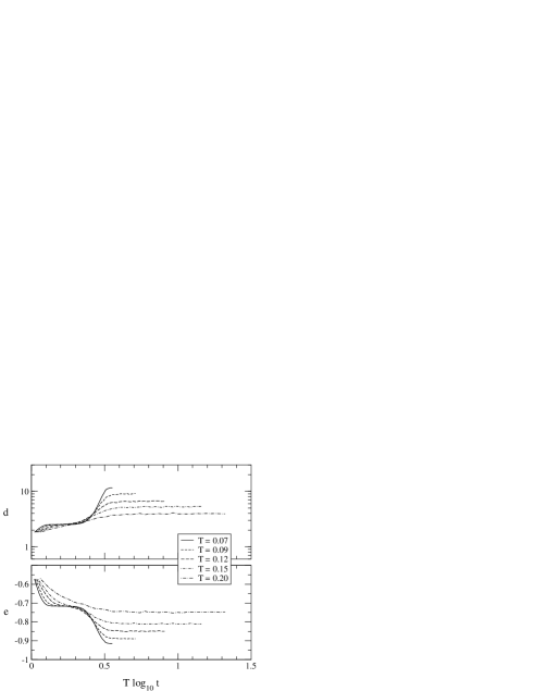
FIG. 24.: Average domain length and energy in the BG model.

Figures 25, 26, 27 and 28 show the correlation function, staggered magnetization and FDT plots of the 1D BG model for the two temperatures $T=0.1$ and $0.09$ and field strength $h_{0}=0.1$.

FIG. 25.: Correlations and staggered magnetization in the BG for $N=10^{4}$, $T=0.10$ and different values of $t_{w}$

From the analysis of the figures the following conclusions can be drawn.

1. After quenching from infinite to low temperature a fast evaporation of occupied boxes occurs after which only a finite fraction of them, approximately $30\%$, survives. Each occupied box contains in average about $3-4$ particles. This process is clearly seen in Fig. 24. The timescale $\tau_{1}\simeq\exp(\beta)/\beta$ has a role similar to the timescale $\tau_{1}$ found in the SCIC model. The aging effects are absent for $t_{w}<\tau_{1}$ but $X<1$ [see Figs. 27 and 28]. The dynamics is again diffusive and similar to the one found for the one-dimensional Ising model [46].

2. For waiting times $t_{w}>\tau_{1}$ the dynamics slows down due to energy barriers. To empty a box a large number of particles must be transferred, a process which is cooperative and involves all the particles in the box. The typical time of this cooperative process is $\tau_{\rm eq}\sim\beta\exp(\beta)$. For waiting times $\tau_{1}<t_{w}<\tau_{eq}$ the system shows strong non-equilibrium effects with a downwards bending of the IRF as a function $C$ similar to what seen in the SCIC model. The origin of this effect is, however, different and follows from the asymmetric response to the staggered field of occupied and empty boxes. Since the field is coupled to empty boxes, the typical time to empty a box is larger than that to occupy an empty one. In other words, when quenching from high (or infinite) temperature boxes are occupied fast and its number converges relatively fast towards the equilibrium value. However, due to the staggered field, the distance among them is far from the equilibrium value and occupied boxes must be rearranged, which is a very slow process. Consequently correlation functions and staggered magnetizations show peculiar humps corresponding to the fast and slow responses.

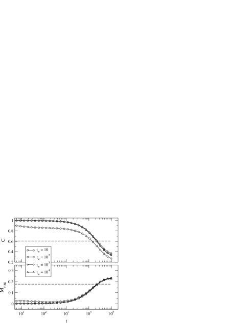
FIG. 26.: The same as Fig. 25 for $T=0.09$.

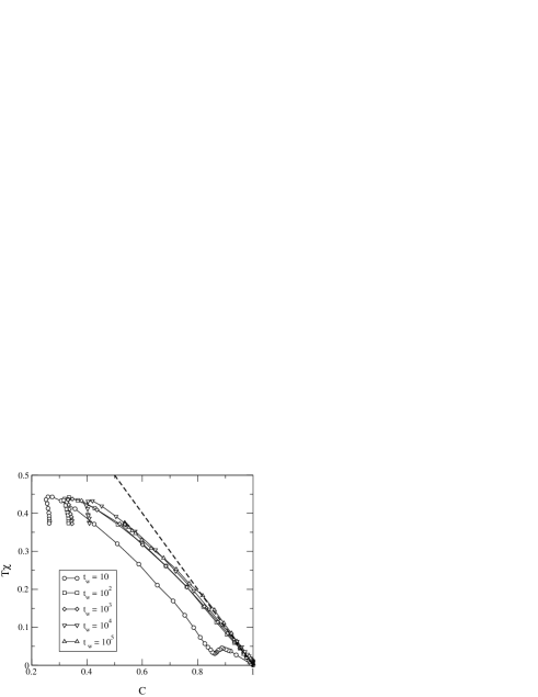
FIG. 27.: FDT plots in the BG for $N=10^{4}$, $T=0.1$ and different values of $t_{w}$.

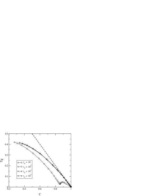
FIG. 28.: The same as Fig. 27 for $T=0.09$.

In conclusion we can say that the strong entropic effects which follows from the large occupation numbers of some boxes at low temperatures, imply that the non-equilibrium behavior of the 1D BG model cannot be well described only in terms of a single length scale $d(t)$. The reason is that although $d(t)$ tells how far the system is from equilibrium it does not contains enough informations to efficiently describe the effects associated with the entropic barriers and the ansatz (22) does not hold.

V Conclusions

In this paper we have studied the dynamics of constrained 1D Ising models. In particular we have focused on a family of constrained kinetic models which interpolate between the symmetrically constrained Ising chain (SCIC) introduced by Fredrickson and Andersen [15] and the asymmetrically constrained Ising chain (ACIC) introduced by Eisinger and Jäckle [21]. For comparison we have also studied the 1D Backgammon model[22] where dynamics is slowed down by the global constraint imposed by the conservation of the particle number. Although these models reproduce some generic features of undercooled liquids there are, however, important differences.

First of all since the class of kinetic constrained models defined in Section II, [see eqs. (1) and (2)] have the same Stillinger-Weber configurational entropy [see Section III] but rather different non-equilibrium behaviors [see Section IV], we conclude that the IS approach is not appropriate for these models. The reason of this failure can be easily understood. Dynamics in coarsening systems is usually described in terms of a growing length scale which measures how close the system is to equilibrium. In this scenario configurations at different times are obviously overlapping since domains at the early times are contained in the larger domains at later times. Consequently the (slow) approach to equilibrium can be described within a geometrical picture in terms of the value of the average domain length.

In undercooled liquids such a length scale probably does not exist and no coarsening takes place in the metastable region. Here the slowing down of the dynamics follows from an activated dynamics in a complex energy landscape composed by many valleys [47]. The SW idea of mapping run-time configurations onto local minima of energy surface (IS) is to provide a statistical description of the valleys. The fact that these valleys are uncorrelated is at the basis of the potentiality of the approach, a result shared by disordered mean-field models for the glass transition such as $p$-spin models [48] or the random energy model [33]. Obviously coarsening plays a role for crystallization processes but we know that the anomalies found in the undercooled regime are also found in disordered models with a crystal state [2, 3], so that the role of the crystal state in the undercooled dynamics can be ignored.

We have critically discussed the SW configurational entropy and its meaning. A conclusion which is difficult to escape from is that any sort of configurational entropy, for example adapted from mean-field theory [14, 17], will have meaning only from a dynamical point of view. Efforts in this direction are the Stillinger and Weber approach itself, the work of Nieuwenhuizen [49], the mean-field scenario by Franz and Virasoso [50] and the very recent approach proposed by Biroli and Kurchan [51].

The description of non-equilibrium dynamics in terms of configurational entropy is valid, in general, if relaxation proceeds via activated jumps between uncorrelated configurations not described by any characteristic length scale. Another possible rephrasing of this conclusion, following the definitions in [36], is to say that models of type I cannot be described in terms of any mean-field like configurational entropy such as the SW approach. Inherent structures and their statistical treatment are only useful for models of type II, category to which structural glasses belong. But as we have shown here, one must be careful in using this classification for models without phase transition but with glassy dynamics when ergodicity is not broken like in ordered (or disordered) ferromagnets. A simple classification based on the infinite time limit of the $Q_{t_{w}}(t)$ seems to be well posed for coarsening ferromagnet-like systems, but for other slow dynamics it may be inappropriate, see some results in Ref. [44]. Still a careful examination of the whole dynamical behavior of $Q_{t_{w}}(t)$, and not only its infinite time limit, may provide useful information to evidentiate how coarsening takes place.

Complementary to this investigation we also made a detailed study of the coarsening behavior of the 1D constrained kinetic models and the 1D Backgammon model analyzing their different non-equilibrium behaviors. Such study confirms theoretical results already present in the literature, but also contains new ones concerning the behavior of the average domain length, in particular for the 1D Backgammon model for which nothing is known, of the magnetization, responses and the violation of fluctuation-dissipation relation. Concerning correlation functions we have found that in all models studied here the $t/t_{w}$ scaling behavior characteristic of mean-field models is not observed. However, when there is a single typical time or length scale, as in the ACIC model, the general scaling (22) and (23) [38] is found. For the SCIC model we have found that the predicted critical timescale $\tau_{1}$ [27] marks the violation of the scaling behavior (22). This peculiar behavior leads to a hump and a broad minimum in the integrated response function and the correlation respectively, leading to a rather unusual fluctuation-dissipation plots. This scenario remains valid for values of $a$ not too far from $1/2$, the region of $a$ close to $1$ (or $0$) is under investigation and will be reported elsewhere. A similar conclusion is valid for the 1D Backgammon model where the presence of entropic barriers induces a second characteristic timescale. In this respect the model with the simpler non-equilibrium dynamics is the ACIC which presents a single timescale and the scaling behavior (22) is well satisfied. This results suggest that the FDT plots to distinguish one glassy scenario from another one must be used with caution. The simple models studied here show interesting FDT plots but no relevant informations can be obtained to interpret the off-equilibrium scenario. Quite probably the only cases where quantities such as configurational entropy or FDT ratio are interesting and meaningful are those where some kind of universality is expected. To this class belong structural glasses. For this case, the Stillinger-Weber decomposition provides a statistical and useful description of some, otherwise inapplicable, mean-field concepts.

In the present research we have tried to clarify the limit of validity of the SW approach to the description of the glassy dynamics. The conclusions that can be drawn from the present study of kinetic constrained models and the Backgammon model can be generalized and we expect that the SW approach will fail to describe any coarsening model. In coarsening models, the information is always contained in a growing domain length which specifies the stage of evolution of microscopic configurations. In undercooled liquids where the simplest coarsening description fails, the SW description is a good alternative which provides the natural link with mean-field ideas.

Appendix A: Closure of dynamical equations

For the constrained kinetic Ising chain the single-spin zero-temperature dynamics s:

$$\dot{\tau}_{i} = -\tau_{i}(a\tau_{i+1}+b\tau_{i-1})$$ (50)

with $a,\,b$ such that $a+b=1$. For $k\geq 0$ we get

$$\frac{d}{dt}(\tau_{i}\cdots\tau_{i+k}) = -a\left(k\,\tau_{i}\cdots\tau_{i+k}+\tau_{i-1}\cdots\tau_{i+k}\right)$$ (52)

$$-b\left(k\,\tau_{i}\cdots\tau_{i+k}+\tau_{i}\cdots\tau_{i+k+1}\right)$$

Following [27] we define the set of correlations,

$$C_{k}(t)=\frac{1}{N}\,\sum_{i=1}^{N}\tau_{i}(t)\tau_{i+1}(t)...\tau_{i+k}(t)$$ (53)

It is simple to see that, for any $a,\,b$ provided that $a+b=1$, the $C_{k}$ satisfy the equations

$$\frac{dC_{k}}{dt} = -k\,C_{k}(t)-C_{k+1}(t)$$ (54)

which are identical to those of FA model computed in [27]. The generating function

$$G(x,t)=\sum_{k=0}^{\infty}\frac{x^{k}}{k!}C_{k}(t)$$

closes the hierarchy yielding the result [27],

$$G(x,t)=G_{0}((1+x)\exp(-t)-1)$$ (55)

with the initial condition $G_{0}(x)=G(x,t=0)$. In the $t\to\infty$ limit (55) yields $C_{k}(\infty)=C_{0}(\infty)\delta_{k,0}$ where,

$$C_{0}(\infty)=\sum_{k=0}^{\infty}\frac{(-1)^{k}}{k!}C_{k}(0)~{}~{}~{}~{}~{}~{}~{}.$$ (56)

Appendix B: Analytical calculation of $P_{IS}(e,T)$

Here we give an analytical derivation of the SW configurational entropy for the constrained Ising chain from the zero-temperature dynamics described in Appendix A. If at $t=0$ the system is in thermal equilibrium at temperature $T$ and the system is large enough the central limit theorem says that the $C_{k}(0)$ are Gaussian distributed variables. Consequently, $C_{0}(\infty)$ is a Gaussian distributed variable with the first two moments given by,

$$\langle C_{0}(\infty)\rangle=\sum_{k=0}^{\infty}\frac{(-1)^{k}}{k!}\langle C_{k}(0)\rangle$$ (57)

$$\langle C_{0}^{2}(\infty)\rangle_{c}=\langle C_{0}^{2}(\infty)\rangle-\langle C_{0}(\infty)\rangle^{2}=\sum_{k=0}^{\infty}\frac{(-1)^{k+l}}{k!l!}\langle C_{k}(0)C_{l}(0)\rangle_{c}$$ (58)

where the subindex $c$ stands for connected correlations. If $m$ stands for the magnetization $m=1/[1+\exp(-\beta)]$ then $C_{k}(0)=(1-m)^{k+1}$ for a thermalized initial condition at temperature $T$. This automatically yields, using (57) the average IS energy $\langle e_{IS}\rangle=\langle C_{0}(\infty)\rangle-1$ yielding,

$$\langle e_{IS}\rangle=(1-m)\exp(m-1)-1~{}~{}~{}~{}.$$ (59)

The computation of the second moment (58) is also straightforward and requires the calculation of $\langle C_{k}C_{l}\rangle_{c}$. A simple calculation gives,

$$\langle C_{k}C_{l}\rangle_{c}=\frac{1}{N}\Bigl{(}(k-l-1+\frac{2}{m})(1-m)^{k+1}-(l+k+1+\frac{2}{m})(1-m)^{k+l+2}\Bigr{)}~{}~{}~{}~{}.$$ (60)

This expression is valid for $k\geq l$ and $k+l+1\leq N$. After some calculations we finally obtain,

$$\langle C_{0}^{2}(\infty)\rangle_{c}=\frac{1}{N}\Bigl{(}(1-m)^{3}\exp(m-1)-\frac{4(1-m)^{2}}{m}\exp(m-1)+\frac{(2-m)(1-m)}{m}I_{0}(2(1-m))$$ (61)

$$+\,2(1-m)^{3}\exp(2m-2)-(\frac{m+2}{m})(1-m)^{2}\exp(2m-2)\Bigr{)}~{}~{}~{}.$$ (62)

where $I_{0}(x)$ is the zeroth order modified Bessel function $I_{0}(x)=\sum_{k=0}^{\infty}\,\frac{x^{2k}}{2^{2k}(k!)^{2}}$. This finally yields for the IS probability distribution (8):

$$P_{IS}(e,T)=\frac{1}{\sqrt{2\pi\langle C_{0}^{2}(\infty)\rangle_{c}}}\exp\Bigl{(}-\frac{(e-\langle e_{IS}\rangle)^{2}}{2\langle C_{0}^{2}(\infty)\rangle_{c}}\Bigr{)}~{}~{}~{}~{}~{}~{}.$$ (63)

From eqs. (59,62) we can directly obtain the configurational entropy in two different ways. One is obtained by exact integration of the IS energy as function of temperature,

$$s_{c}(e)=\int_{0}^{T}\frac{de(T)}{dT}\frac{dT}{T}$$ (64)

where $e(T)$ is given by the expression (59). The other is obtained by integrating the fluctuations,

$$s_{c}(e)=\int_{0}^{T}\frac{\langle C_{0}^{2}(\infty)\rangle_{c}}{T^{3}}\,dT$$ (65)

According to (8) both expressions should coincide when the term $f(\beta,e)$ in (8) is independent of the energy $e$. This is generally not true and expressions (15), (65) are different. The interesting remark is that, in the limit $T\to 0$ both expressions (15), (65) and the fix-point approximation (11) coincide to first order in $T$. The reason is that the SW configurational entropy has full meaning in the limit where $s_{c}$ goes to zero and the IS-basins are very narrow containing few configurations.

REFERENCES

- [1] Complex behavior in glassy systems, Proceedings of the XIV Sitges Conference 1996, Springer-Verlag, Ed. M. Rubí and C. Perez-Vicente; C. A. Angell, Science 267, 1924 (1995).
- [2] J. P. Bouchaud and M. Mezard, J. Physique I, 4, 1109 (1994)
- [3] E. Marinari, G. Parisi and F. Ritort, J. Phys. A (Math. Gen.) 27, 7615 (1994); J. Phys. A (Math. Gen.) 27, 7647 (1994).
- [4] W. Kob, C. Donati, S. J. Plimpton, P. H. Poole and S. C. Glotzer, Phys. Rev. Lett. 79, 2827 (1997); C. Donati, J. F. Douglas, W. Kob, S. J. Plimpton, P. H. Poole and S. C. Glotzer, Phys. Rev. Lett. 80, 2338 (1998); B. Doliwa and A. Heuer, Phys. Rev. Lett. 80, 4915 (1998).
- [5] G. Parisi, J. Phys. Chem. 103, 4128 (1999)
- [6] J. P. Bouchaud, Aging in glassy systems: new experiments, simple models, and open questions Preprint cond-mat/9910387
- [7] J. Hammann, E. Vincent, V. Dupuis, M. Alba, M. Ocio, J.-P. Bouchaud, Preprint cond-mat 9911269
- [8] N. Menon and S. R. Nagel, Phys. Rev. Lett. 74, 1230 (1995); R. L. Leheny, N. Menon, S. R. Nagel, D. L. Price, K. Suzuya and P. Thiyagarajan, J. Chem. Phys. 105, 7783 (1996).
- [9] S. Franz and G. Parisi, On nonlinear susceptibility in supercooled liquids, Preprint cond-mat/0005095
- [10] W. Gotze, in Liquid, Freezing and the Glass Transition, 1989 Les Houches Lectures, Ed. by J. P. Hansen, D. Levesque and J. Zinn-Justin (North-Holland, Amsterdam, 1989).
- [11] F. H. Stillinger and T. A. Weber, Phys. Rev. A 25, 978 (1982)
- [12] J. H. Gibbs and E. A. Di Marzio, J. Chem. Phys. 28, 373 (1968); G. Adams and J. H. Gibbs, J. Chem. Phys. 43, 139 (1965).
- [13] T. R. Kirkpatrick and D. Thirumalai, Phys. Rev. Lett. 58, 2091 (1987); T.R. Kirkpatrick and P.G. Wolynes, Phys. Rev. B36, 8552 (1987).
- [14] M. Mezard and G. Parisi, Phys. Rev. Lett. 82, 747 (1998); J. Chem. Phys. 111, 1076 (1999).
- [15] G. H. Fredrickson and H. C. Andersen, Phys. Rev. Lett 53, 1244 (1984); G. H. Fredrickson and H. C. Andersen, J. Chem. Phys. 83, 5822 (1985); G. H. Fredrickson and S. A. Brawer, J. Chem. Phys. 84, 3351 (1986);
- [16] G. H. Fredrickson, Ann. Rev. Phys. Chem. 39, 149 (1988).
- [17] M. Mezard, Physica A, 265, 352 (1999); B. Coluzzi, M. Mezard, G. Parisi and P. Verrochio, J. Chem. Phys. 111, 9039 (1999).
- [18] F. Sciortino W. Kob and P. Tartaglia, Phys. Rev. Lett. 83, 3214 (1999).
- [19] W. Kob, F. Sciortino and P. Tartaglia, cond-mat 9905090
- [20] A. Crisanti and F. Ritort, Potential energy landscape of finite-size mean-field models for glasses Preprint cond-mat 9907499 to appear in Europhys Letters and Activated processes and Inherent Structure dynamics of finite-size mean-field models for glasses Preprint cond-mat 9911226.
- [21] J. Jäckle and S. Eisinger, Z. Phys. B84, 115 (1991); S. Eisinger and J. Jackle, J. Stat. Phys. 73, 643 (1993).
- [22] F. Ritort, Phys. Rev. Lett. 75, 1190 (1995)
- [23] J. Reiter and J. Jackle, Physica A 215, 311 (1995).
- [24] M. Schulz and S. Trimper, J. Stat. Phys. 94, 173 (1999).
- [25] F. Mauch and J. Jackle, Physica A 262, 98 (1999).
- [26] P. Sollich and M. R. Evans, Phys. Rev. Lett. 83, 3238 (1999)
- [27] E. Follana and F. Ritort, Phys. Rev. B 54, 930 (1996)
- [28] C. Godreche , J. P. Bouchaud and M. Mezard, J. Phys. A 28, L603 (1995); S. Franz and F. Ritort, J. Stat. Phys. 85, 131 (1996).
- [29] S. Franz and F. Ritort, J. Phys. A 30, L359 (1997)
- [30] C. Godreche and J. M. Luck, J. Phys. A 30, 6245 (1997); ibid, J. Phys. A 32, 6033 (1999)
- [31] S. F. Edwards and A. Mehta, J. Phys. (France) 50, 2489 (1989).
- [32] R. Monasson and O. Pouliquen, Physica A 236, 395 (1997).
- [33] B. Derrida, Phys, Rev. B, 24 (1981) 2613.
- [34] G. Biroli and R. Monasson, Europhys. Lett., 50, 155 (2000).
- [35] C. Beck and F. Schlögl, Thermodynamics of chaotic systems:an introduction, Cambridge Nonlinear Science Series 4, Cambridge University Press, 1993.
- [36] A. Barrat, R. Burioni and M. Mezard, J. Phys. A (Math. Gen.) 29, 1311 (1996).
- [37] A. Crisanti and F. Ritort, unpublished.
- [38] A. J. Bray, Adv. Phys. 43, 357 (1994)
- [39] J. P. Bouchaud, L. F. Cugliandolo, J. Kurchan and M. Mezard in Spin Glasses and Random Fields Ed. by A. P. Young, World Scientific, Singapore, 1998.
- [40] L. Berthier, J. L. Barrat and J. Kurchan, Eur. Phys. J. B 11, 635 (1999)
- [41] F. Ricci-Tersenghi and F. Ritort, Absence of aging in the remanent magnetization in Migdal-Kadanoff spin glasses, Preprint cond-mat 9910390 to appear in J. Phys. A
- [42] L. F. Cugliandolo and J. Kurchan, J. Phys. A (Math. Gen.) 27, 5749 (1994); S. Franz and H. Rieger, J. Stat. Phys. 79, 749 (1995); E. Marinari, G. Parisi, F. Ricci-Tersenghi, J. J. Ruiz-Lorenzo, J. Phys. A: Math. Gen. 31, 2611 (1998).
- [43] A. Barrat, Phys. Rev. E 57, 3629 (1998).
- [44] D. Alvarez, S. Franz and F. Ritort, Phys. Rev. B 54, 9756 (1996); M. R. Swift, H. Bokil, R. D. M. Travasso, A. J. Bray, Novel glassy behavior in a ferromagnetic p-spin model Preprint cond-mat 0003384.
- [45] The domain length grows as . Indeed if time is rescaled by all curves in Fig. 7 collapse onto a single curve. We are grateful to Peter Sollich for calling our attention to this point.
- [46] C. Godreche and J. M. Luck, J. Phys. A 33, 1151 (2000); E. Lippiello and M. Zannetti, Fluctuation dissipation ratio in the one dimensional kinetic Ising model, Preprint cond-mat/0001103
- [47] F. H. Stillinger, Science 26, 1935 (1995).
- [48] In that case it is know that despite metastable states are pairwise randomly uncorrelated there are non trivial-three state correlations. See, A. Cavagna, I. Giardina and G. Parisi, J. Phys. A (Math. Gen.) 30, 4449 (1997); J. Phys. A (Math. Gen.) 30, 7021 (1997); A. Barrat and S. Franz, J. Phys. A (Math. Gen.) 31, L119 (1998).
- [49] Th. M. Nieuwenhuizen, J. Phys. A 31, L201 (1998); Preprint cond-mat9811390
- [50] S. Franz and M. Virasoro, J. Phys. A (Math. Gen.) 33, 891 (2000).
- [51] G. Biroli and J. Kurchan, cond-mat/0005499
- [52] J. P. Garrahan and M. E. J. Newman, cond-mat/0007372