Charge Current Density from the Scattering Matrix

Abstract

A method to derive the charge current density and its quantum mechanical correlation from the scattering matrix is discussed for quantum scattering systems described by a time-dependent Hamiltonian operator. The current density and charge density are expressed with the help of functional derivatives with respect to the vector potential and the electric potential. A condition imposed by the requirement that these local quantities are gauge invariant is considered. Our formulas lead to a direct relation between the local density of states and the total current density at a given energy. To illustrate the results we consider, as an example, a chiral ladder model.

$\langle$ Introduction $\rangle$ The scattering matrix gives an important starting point in descriptions of quantum transport phenomena. It connects the incoming current amplitudes to the outgoing current amplitudes, and is calculated from the Hamiltonian operator by the Møller operator or the Green function method [1]. We can obtain information about global characteristics in systems from the scattering matrix directly. For example, the Landauer formula gives a method to calculate the conductance from transmission amplitudes as components of the scattering matrix [2, 3, 4, 5, 6, 7]. The Friedel sum rule connects the density of states to the scattering matrix [8, 9], so that it is in principle possible to calculate any equilibrium statistical mechanical quantity from the scattering matrix [10]. We can also derive an expression of the persistent current in open conductors caused by a magnetic flux [11], or the shot noise [12, 13] from the scattering matrix.

It should be emphasized that the scattering matrix even gives information about local characteristics in systems. We consider one-particle and time-dependent Hamiltonian systems. First, the charge current density $\mbox{\boldmath$J$}_{n}(\mbox{\boldmath$x$},t)$ at position $x$ and time $t$ generated by the particle incident in a state with the quantum number $n$ is connected to the scattering matrix $S=(S_{nn^{\prime}})$ as

$$\mbox{\boldmath$J$}_{n}(\mbox{\boldmath$x$},t)=\frac{c}{2\pi i}\sum_{n^{\prime}}S_{n^{\prime}n}^{*}\frac{\delta S_{n^{\prime}n}}{\delta\mbox{\boldmath$A$}(\mbox{\boldmath$x$},t)}$$ (1)

where $\mbox{\boldmath$A$}(\mbox{\boldmath$x$},t)$ is the vector potential and $c$ is the velocity of light. In this Letter we call this quantity the ”injected current density”. Eq. (1) is the main result of this Letter. Second, the probability density $\rho_{n}(\mbox{\boldmath$x$},t)$ of the state caused by the incident particle with the quantum number $n$ is given by

$$\rho_{n}(\mbox{\boldmath$x$},t)=-\frac{1}{2\pi i}\sum_{n^{\prime}}S_{n^{\prime}n}^{*}\frac{\delta S_{n^{\prime}n}}{\delta U(\mbox{\boldmath$x$},t)}$$ (2)

with the potential $U(\mbox{\boldmath$x$},t)$. The probability density $\rho_{n}(\mbox{\boldmath$x$},t)$ also has been called the ”injectivity” and can be regarded as the density of states with a preselection of the incident channel. Eq. (2) in the time-independent Hamiltonian case has been used in treatments of the electron-electron interaction using a self-consistent potential [14, 15, 16, 17]. In this Letter we give a new derivation of this formula and generalize it to the time-dependent Hamiltonian case.

Our technique to derive Eqs. (1) and (2) also can be used to arrive at quantum mechanical correlation functions of local quantities from the scattering matrix. For example we show that the quantum mechanical correlation $C_{n}^{\scriptscriptstyle(\mu\nu)}(\mbox{\boldmath$x$},\mbox{\boldmath$x$}^{\prime};t)$ between the $\mu$-th charge current density component at position $x$ and the $\nu$-th charge current density component at position $\mbox{\boldmath$x$}^{\prime}$ at the same time $t$ is given by

$$C_{n}^{\scriptscriptstyle(\mu\nu)}(\mbox{\boldmath$x$},\mbox{\boldmath$x$}^{\prime};t)=\frac{c^{2}\hbar}{2\pi}\sum_{n^{\prime}}\mbox{Re}\left\{\frac{\delta S_{n^{\prime}n}^{*}}{\delta A^{\scriptscriptstyle(\mu)}(\mbox{\boldmath$x$},t)}\frac{\delta S_{n^{\prime}n}}{\delta A^{\scriptscriptstyle(\nu)}(\mbox{\boldmath$x$}^{\prime},t)}\right\}$$ (3)

(4)

where $A^{\scriptscriptstyle(\mu)}(\mbox{\boldmath$x$},t)$ is the $\mu$-th component of the vector potential.

Our formulas include the vector potential and the potential explicitly, so we have to discuss the gauge invariance. We show Eqs. (1 - 2) and (4) to be gauge invariant, and derive conditions which should be satisfied by locally gauge invariant quantities.

In the time-dependent Hamiltonian system an energy of an outgoing particle can be different from the energy of the corresponding incoming particle, and the scattering matrix element $S_{nn^{\prime}}$ describes a transition to such a different energy. On the other hand, if we consider only time-independent Hamiltonian cases, the problem becomes simpler, because the scattering matrix is decomposed into the scattering matrices restricted to the energy shells. Using this feature we obtain a relation between the local density of states and the total current density defined by the sum of the injected current density $\mbox{\boldmath$J$}_{n}(\mbox{\boldmath$x$},t)$ with respect to the suffix $n$ satisfying the condition $E_{n}=E$ at energy $E$.

As a simple example we investigate a ladder model with a directionality, namely a chiral ladder model, termed a ”quantum rail road” in Ref. [18]. We verify the formula (1) for this model calculating separately the current density and the scattering matrix.

$\langle$ Injected current density and injectivity $\rangle$ We start from the time-dependent Hamiltonian operator $\hat{H}(t)$ in the quantum scattering system. The dynamics of the system is described by the Schrödinger equation using this Hamiltonian operator. We decompose the total Hamiltonian operator $\hat{H}(t)$ into the asymptotic Hamiltonian operator $\hat{H}_{0}$ and the scattering operator $\hat{H}_{1}(t)$; $\hat{H}(t)=\hat{H}_{0}+\hat{H}_{1}(t)$. The operator $\hat{H}_{0}$ is chosen to be the Hamiltonian operator which describes incoming and outgoing particles in the asymptotic regions. We assume that $\hat{H}_{0}$ is a time-independent operator determined uniquely. Besides, the system described by the Hamiltonian operator $\hat{H}(t)$ or $\hat{H}_{0}$ is assumed to have no bound state. Below we use the coordinate representation for any operator and take $x$ as the coordinate of particles. Under these conditions the scattering matrix element $S_{nn^{\prime}}$ is given by

$$S_{nn^{\prime}}=\lim_{t_{2}\rightarrow+\infty}\lim_{t_{1}\rightarrow-\infty}\int d\mbox{\boldmath$x$}\;\Phi_{n}(\mbox{\boldmath$x$})^{*}\hat{U}(t_{2},t_{1})\Phi_{n^{\prime}}(\mbox{\boldmath$x$})$$ (5)

where $\hat{U}(t_{2},t_{1})$ is the time evolution operator $\exp\{i\hat{H}_{0}t_{2}/\hbar\}$$\cdot\vec{T}\exp\{-i\int_{t_{1}}^{t_{2}}dt\hat{H}(t)/\hbar\}$ $\cdot\exp\{-i$ $\hat{H}_{0}t_{1}/\hbar\}$ in the interaction picture with $\vec{T}$ being the positive time-ordering operator, and $\Phi_{n}(\mbox{\boldmath$x$})$ is the eigenstate of the operator $\hat{H}_{0}$ corresponding to the energy eigenvalue $E_{n}$. Here the limits $t_{1}\rightarrow-\infty$ and $t_{2}\rightarrow+\infty$ are defined by $\lim_{t\rightarrow\pm\infty}X(t)\equiv\lim_{\epsilon\rightarrow+0}(\pm\epsilon)\int_{0}^{\pm\infty}dt^{\prime}e^{\mp\epsilon t^{\prime}}$$X(t^{\prime})$ for any function $X(t)$ of $t$ [1]. The set $\{\Phi_{n}(\mbox{\boldmath$x$})\}_{n}$ of the eigenstates of the operator $\hat{H}_{0}$ is chosen to satisfy the orthonormality condition and the completeness relation. The scattering matrix $S=(S_{nn^{\prime}})$ is shown to be an unitary matrix; $S^{\dagger}S=SS^{\dagger}=I$.

For simplicity we consider the one-particle system. The total Hamiltonian operator $\hat{H}(t)$ and the operator $\hat{H}_{0}$ are represented as $(-i\hbar\partial/\partial\mbox{\boldmath$x$}-q\mbox{\boldmath$A$}(\mbox{\boldmath$x$},t)/c)^{2}/(2m)+U(\mbox{\boldmath$x$},t)+U_{0}(\mbox{\boldmath$x$})$ and $-(\hbar^{2}/(2m))\partial^{2}/\partial\mbox{\boldmath$x$}^{2}+U_{0}(\mbox{\boldmath$x$})$, respectively, where $m$ is the mass of the particle, $q$ is the charge of the particle, $\mbox{\boldmath$A$}(\mbox{\boldmath$x$},t)$ is the vector potential, and $U(\mbox{\boldmath$x$},t)$ is the external potential (plus the induced potential by the interaction of particles), and $U_{0}(\mbox{\boldmath$x$})$ is the confinement potential. We consider a functional derivative $\delta^{\scriptscriptstyle(t)}\hat{S}_{nn^{\prime}}$ of the scattering matrix element with respect to the vector potential $\mbox{\boldmath$A$}(\mbox{\boldmath$x$},t)$ or the potential $U(\mbox{\boldmath$x$},t)$ at time $t$, using the notation $\delta^{\scriptscriptstyle(t)}=\delta/\delta\mbox{\boldmath$A$}(\mbox{\boldmath$x$},t)$ or $\delta/\delta U(\mbox{\boldmath$x$},t)$. Using the expression (5) of the scattering matrix elements we obtain a general relation

$$\frac{1}{2\pi i}\sum_{n^{\prime}}S_{n^{\prime}n}^{*}(\delta^{\scriptscriptstyle(t)}S_{n^{\prime}n})=-\left\langle\;\int_{-\infty}^{\infty}dt^{\prime}\;\delta^{\scriptscriptstyle(t)}\hat{H}_{1}(t^{\prime})\;\right\rangle_{n}^{\scriptscriptstyle(t)}.$$ (6)

Here the notation $\langle\,\cdots\,\rangle_{n}^{\scriptscriptstyle(t)}$ means the expectation value taken with the scattering state of the quantum number $n$, namely $\langle\,\hat{X}\,\rangle_{n}^{\scriptscriptstyle(t)}\equiv\int d\mbox{\boldmath$x$}\Psi_{n}(\mbox{\boldmath$x$},t)^{*}\hat{X}\Psi_{n}(\mbox{\boldmath$x$},t)$ $/(2\pi\hbar)$ for any operator $\hat{X}$, where $\Psi_{n}(\mbox{\boldmath$x$},t)$ is a solution of the Schrödinger equation using the total Hamiltonian operator $\hat{H}(t)$ and is defined by $\Psi_{n}(\mbox{\boldmath$x$},t)\equiv\lim_{t_{1}\rightarrow-\infty}\vec{T}\exp\{-i\int_{t_{1}}^{t}dt^{\prime}\;\hat{H}(t^{\prime})/\hbar\}\cdot\exp\{-iE_{n}t_{1}/\hbar\}\Phi_{n}(\mbox{\boldmath$x$})$. The derivation of Eq. (6) is given by using the completeness relation of the set $\{\Phi_{n}(\mbox{\boldmath$x$})\}_{n}$, the property $\hat{U}(t_{2},t_{1})=\hat{U}(t_{2},t)\hat{U}(t,t_{1})$ of the time evolution operator and the relation $\delta^{\scriptscriptstyle(t)}\hat{U}(t_{2},t_{1})=\hat{U}(t_{2},t)\cdot\exp{\{i\hat{H}_{0}t/\hbar\}}\cdot\{(-i/\hbar)\;\int_{-\infty}^{\infty}dt^{\prime}\delta^{\scriptscriptstyle(t)}\hat{H}_{1}(t^{\prime})\}\cdot\exp{\{-i\hat{H}_{0}t/\hbar\}}\cdot\hat{U}(t,t_{1})$ in $t_{1}<t<t_{2}$. Eq. (6) is a key result of this Letter. We introduce the injected current density $\mbox{\boldmath$J$}_{n}(\mbox{\boldmath$x$},t)$ and the injectivity $\rho_{n}(\mbox{\boldmath$x$},t)$ as

$$\mbox{\boldmath$J$}_{n}(\mbox{\boldmath$x$},t)\equiv\left\langle\;\hat{\mbox{\boldmath$J$}}(\mbox{\boldmath$x$},t)\;\right\rangle_{n}^{\scriptscriptstyle(t)},\;\;\;\;\;\;\rho_{n}(\mbox{\boldmath$x$},t)\equiv\left\langle\;\hat{\rho}(\mbox{\boldmath$x$})\;\right\rangle_{n}^{\scriptscriptstyle(t)}$$ (7)

using the charge current density operator $\hat{\mbox{\boldmath$J$}}(\mbox{\boldmath$r$},t)\equiv q\hat{\mbox{\boldmath$v$}}(t)\star\delta(\mbox{\boldmath$x$}-\mbox{\boldmath$r$})$ with $\hat{\mbox{\boldmath$v$}}(t)$ being the velocity operator $(-i\hbar\partial/\partial\mbox{\boldmath$x$}-q\mbox{\boldmath$A$}(\mbox{\boldmath$x$},t)/c)/m$ and the multiplication $\star$ being the symmetrized product, and using the probability density operator $\hat{\rho}(\mbox{\boldmath$r$})\equiv\delta(\mbox{\boldmath$x$}-\mbox{\boldmath$r$})$. Eqs. (1) and (2) are derived from Eq. (6), using the relations $\int_{-\infty}^{\infty}dt^{\prime}\delta\hat{H}_{1}(t^{\prime})/\delta\mbox{\boldmath$A$}(\mbox{\boldmath$x$},t)=-\hat{\mbox{\boldmath$J$}}(\mbox{\boldmath$x$},t)/c$ and $\int_{-\infty}^{\infty}dt^{\prime}\delta\hat{H}_{1}(t^{\prime})/\delta U(\mbox{\boldmath$x$},t)=\hat{\rho}(\mbox{\boldmath$x$})$.

$\langle$ Current density correlation $\rangle$ We consider functional derivatives $\delta_{j}^{\scriptscriptstyle(t)}S_{nn^{\prime}}$, $j=1,2$ of the scattering matrix element with respect to the vector potential $\mbox{\boldmath$A$}(\mbox{\boldmath$x$},t)$ or the potential $U(\mbox{\boldmath$x$},t)$ at time $t$. Using Eq. (5) we obtain another general relation

$$\frac{\hbar}{2\pi}\sum_{n^{\prime}}\left(\delta_{1}^{\scriptscriptstyle(t)}S_{n^{\prime}n}^{*}\right)\left(\delta_{2}^{\scriptscriptstyle(t)}S_{n^{\prime}n}\right)$$ (8)

$$=\left\langle\;\left(\int_{-\infty}^{\infty}dt^{\prime}\delta_{1}^{\scriptscriptstyle(t)}\hat{H}_{1}(t^{\prime})\right)\left(\int_{-\infty}^{\infty}dt^{\prime\prime}\delta_{2}^{\scriptscriptstyle(t)}\hat{H}_{1}(t^{\prime\prime})\right)\;\right\rangle_{n}^{\scriptscriptstyle(t)}.$$ (9)

Using Eq. (9) we obtain Eq. (4). Here the quantum mechanical current density correlation $C_{n}^{\scriptscriptstyle(\mu\nu)}(\mbox{\boldmath$x$},\mbox{\boldmath$x$}^{\prime};t)$ is defined by

$$C_{n}^{\scriptscriptstyle(\mu\nu)}(\mbox{\boldmath$x$},\mbox{\boldmath$x$}^{\prime};t)\equiv\left\langle\;\hat{J}^{\scriptscriptstyle(\mu)}(\mbox{\boldmath$x$},t)\star\hat{J}^{\scriptscriptstyle(\nu)}(\mbox{\boldmath$x$}^{\prime},t)\;\right\rangle_{n}^{\scriptscriptstyle(t)}$$ (10)

where $\hat{J}^{\scriptscriptstyle(\mu)}(\mbox{\boldmath$x$},t)$ is the $\mu$-th component of the charge current density operator. It should be noted that the average $\langle\,\cdots\,\rangle_{n}^{\scriptscriptstyle(t)}$ taken in the correlation (10) includes only the quantum mechanical average, but does not include the thermo-statistical average.

In similar ways we can obtain other quantum mechanical correlation functions $\langle\,\hat{J}^{\scriptscriptstyle(\nu)}(\mbox{\boldmath$x$},t)\star\hat{\rho}(\mbox{\boldmath$x$}^{\prime})\,\rangle_{n}^{\scriptscriptstyle(t)}$ and $\langle\,\hat{\rho}(\mbox{\boldmath$x$})\star\hat{\rho}(\mbox{\boldmath$x$}^{\prime})\,\rangle_{n}^{\scriptscriptstyle(t)}$ from the scattering matrix.

$\langle$ Gauge invariance $\rangle$ The gauge transformation of the electric potential $\phi(\mbox{\boldmath$x$},t)$ and the vector potential $\mbox{\boldmath$A$}(\mbox{\boldmath$x$},t)$ is represented as $\phi(\mbox{\boldmath$x$},t)\rightarrow\phi(\mbox{\boldmath$x$},t)+\Delta\phi(\mbox{\boldmath$x$},t)$ and $\mbox{\boldmath$A$}(\mbox{\boldmath$x$},t)\rightarrow\mbox{\boldmath$A$}(\mbox{\boldmath$x$},t)+\Delta\mbox{\boldmath$A$}(\mbox{\boldmath$x$},t)$ with $\Delta\phi(\mbox{\boldmath$x$},t)\equiv-(1/c)\partial\varphi(\mbox{\boldmath$x$},t)/\partial t$ and $\Delta\mbox{\boldmath$A$}(\mbox{\boldmath$x$},t)\equiv\partial\varphi(\mbox{\boldmath$x$},t)/\partial\mbox{\boldmath$x$}$ using a function $\varphi(\mbox{\boldmath$x$},t)$ of $x$. The electric and magnetic fields are invariant under the gauge transformation. Using that the Schrödinger equation is gauge invariant, we can show that the $\mu$-th component $J_{n}^{\scriptscriptstyle(\mu)}(\mbox{\boldmath$x$},t)$ of the injected current density is also gauge invariant, meaning that the formula (1) is gauge invariant.

The fact that the injected current density is gauge invariant is also represented as

$$\int dt^{\prime}\;\int d\mbox{\boldmath$x$}^{\prime}\;\left\{\frac{\delta J_{n}^{\scriptscriptstyle(\mu)}(\mbox{\boldmath$x$},t)}{\delta\phi(\mbox{\boldmath$x$}^{\prime},t^{\prime})}\;\Delta\phi(\mbox{\boldmath$x$}^{\prime},t^{\prime})\right.$$ (11)

$$\hskip 76.82234pt+\left.\frac{\delta J_{n}^{\scriptscriptstyle(\mu)}(\mbox{\boldmath$x$},t)}{\delta\mbox{\boldmath$A$}(\mbox{\boldmath$x$}^{\prime},t^{\prime})}\cdot\Delta\mbox{\boldmath$A$}(\mbox{\boldmath$x$}^{\prime},t^{\prime})\right\}=0.$$ (12)

A change $\delta\phi(\mbox{\boldmath$x$},t)$ of the electric potential $\phi(\mbox{\boldmath$x$},t)$ modifies the potential $U(\mbox{\boldmath$x$},t)$ as $\delta U(\mbox{\boldmath$x$},t)=q\delta\phi(\mbox{\boldmath$x$},t)$. Moreover Eq. (12) should be satisfied for any function $\varphi(\mbox{\boldmath$x$},t)$ which is zero at the boundary of the integral of the left-hand side of Eq. (12). Using these facts and the partial integrals in Eq. (12) we obtain

$$\frac{q}{c}\frac{\partial}{\partial t^{\prime}}\frac{\delta J_{n}^{\scriptscriptstyle(\mu)}(\mbox{\boldmath$x$},t)}{\delta U(\mbox{\boldmath$x$}^{\prime},t^{\prime})}+\frac{\partial}{\partial\mbox{\boldmath$x$}^{\prime}}\cdot\frac{\delta J_{n}^{\scriptscriptstyle(\mu)}(\mbox{\boldmath$x$},t)}{\delta\mbox{\boldmath$A$}(\mbox{\boldmath$x$}^{\prime},t^{\prime})}=0.$$ (13)

Eq. (13) represents a condition for the injected current density imposed by its gauge invariance. Similarly, the formulas (2) and (4) are gauge invariant, and the injectivity $\rho_{n}(\mbox{\boldmath$x$},t)$ satisfies an equation similar to Eq. (13).

$\langle$ Total current density and local density of states in the time-independent Hamiltonian system $\rangle$ Now, we consider the time-independent Hamiltonian case. In this case the injected current density and the injectivity are independent of time $t$. Moreover the state $\Psi_{n}(\mbox{\boldmath$x$},t)$ used to define the average $\langle\,\cdots\,\rangle_{n}^{\scriptscriptstyle(t)}$ can be replaced by the state $\bar{\Psi}_{n}(\mbox{\boldmath$x$})\equiv\{1+\hat{G}(E_{n})\hat{H}_{1}\}\Phi_{n}(\mbox{\boldmath$x$})$ using the Green operator $\hat{G}(E)\equiv\lim_{\epsilon\rightarrow+0}(E-\hat{H}+i\epsilon)^{-1}$. The state $\bar{\Psi}_{n}(\mbox{\boldmath$x$})$ is the eigenstate of the total Hamiltonian operator $\hat{H}$ corresponding to the eigenvalue $E_{n}$ and satisfies the Lippmann-Schwinger equation. One of the important features in the time-independent Hamiltonian system is that the scattering matrix element $S_{nn^{\prime}}$ takes a non-zero value only in the case of $E_{n}=E_{n^{\prime}}$. Therefore, in the formulas (1) and (2) we can replace the full scattering matrix element $S_{n^{\prime}n}$ with the matrix element ${\cal{S}}_{l^{\prime}l}(E_{n})$ of the scattering matrix ${\cal{S}}(E_{n})$ restricted to the energy shell of energy $E_{n}$, and exchange the sum of the quantum number $n^{\prime}$ with the sum of the channel number $l^{\prime}$.

It is important to note a difference between the time-dependent and time-independent Hamiltonian cases in our formulas. In the time-dependent Hamiltonian case the functional derivative $\delta S_{nn^{\prime}}/\delta\mbox{\boldmath$A$}(\mbox{\boldmath$x$},t)$ is given by $\delta S_{nn^{\prime}}=\int d\mbox{\boldmath$x$}\int dt$ $(\delta S_{nn^{\prime}}/\delta\mbox{\boldmath$A$}(\mbox{\boldmath$x$},t))\delta\mbox{\boldmath$A$}(\mbox{\boldmath$x$},t)$. On the other hand, in the time-independent Hamiltonian case the functional derivative $\delta{\cal{S}}_{ll^{\prime}}(E)/\delta\mbox{\boldmath$A$}(\mbox{\boldmath$x$})$ is given by $\delta{\cal{S}}_{ll^{\prime}}(E)=\int d\mbox{\boldmath$x$}(\delta{\cal{S}}_{ll^{\prime}}(E)/\delta\mbox{\boldmath$A$}(\mbox{\boldmath$x$}))\delta\mbox{\boldmath$A$}(\mbox{\boldmath$x$})$, which does not include the time integral like in the time-dependent Hamiltonian case. This difference appears in the current density correlation formula (4), where a simple exchange of the scattering matrix element $S_{nn^{\prime}}$ and the vector potential $\mbox{\boldmath$A$}(\mbox{\boldmath$x$},t)$ with the on-shell scattering matrix element ${\cal{S}}_{ll^{\prime}}(E)$ and the vector potential $\mbox{\boldmath$A$}(\mbox{\boldmath$x$})$, respectively, is not allowed to obtain its time-independent Hamiltonian version. However we can obtain the time-independent Hamiltonian versions of the injected current density formula (1) and the injectivity formula (2) by such a simple exchange. This technical point is better considered in a separate paper.

We proceed to consider the total current density $\mbox{\boldmath$J$}(E,\mbox{\boldmath$x$})$ and the local density of states $\rho(E,\mbox{\boldmath$x$})$ defined by

$$\mbox{\boldmath$J$}(E,\mbox{\boldmath$x$})\equiv\!\!\!\!\!\!\!\!\sum_{\begin{array}[]{c}{\scriptstyle n}\\ \left({\scriptstyle E_{n}=E}\right)\end{array}}\!\!\!\!\mbox{\boldmath$J$}_{n}(\mbox{\boldmath$x$}),\;\;\;\;\;\;\rho(E,\mbox{\boldmath$x$})\equiv\!\!\!\!\!\!\!\!\sum_{\begin{array}[]{c}{\scriptstyle n}\\ \left({\scriptstyle E_{n}=E}\right)\end{array}}\!\!\!\!\rho_{n}(\mbox{\boldmath$x$}).$$ (18)

Eqs. (1) and (2) lead to

$$\mbox{\boldmath$J$}(E,\mbox{\boldmath$x$})=\frac{c}{\pi}\frac{\delta\theta_{\!f}(E)}{\delta\mbox{\boldmath$A$}(\mbox{\boldmath$x$})},\;\;\;\;\;\;\rho(E,\mbox{\boldmath$x$})=-\frac{1}{\pi}\frac{\delta\theta_{\!f}(E)}{\delta U(\mbox{\boldmath$x$})}$$ (19)

where $\theta_{\!f}(E)$ is called ”Friedel phase” [19] and is defined by $\theta_{\!f}(E)\equiv(1/(2i))\ln\mbox{Det}\{{\cal{S}}(E)\}$. It may be noted that using the first equation in Eq. (19) the relation $\mbox{\boldmath$J$}(E,\mbox{\boldmath$x$})=-\mbox{\boldmath$J$}(E,\mbox{\boldmath$x$})|_{\mbox{\boldmath${\scriptstyle A}$}\rightarrow-\mbox{\boldmath${\scriptstyle A}$}}$ is obtained under the condition $S_{nn^{\prime}}=S_{n^{\prime}n}|_{\mbox{\boldmath${\scriptstyle A}$}\rightarrow-\mbox{\boldmath${\scriptstyle A}$}}$. The second formula in Eq. (19) have already been used in some works [14, 15, 16, 17, 20]. It follows from Eq. (19) that

$$\frac{\delta\mbox{\boldmath$J$}(E,\mbox{\boldmath$x$}^{\prime})}{\delta U(\mbox{\boldmath$x$})}=-c\frac{\delta\rho(E,\mbox{\boldmath$x$})}{\delta\mbox{\boldmath$A$}(\mbox{\boldmath$x$}^{\prime})}.$$ (20)

This equation shows a connection of the current density to the local density of states.

The total current density $\mbox{\boldmath$J$}(E,\mbox{\boldmath$x$})$ takes a non-zero value in some important phenomena, such as edge currents in the quantum hall effect, persistent currents caused by a magnetic flux and so on. Earlier work [11] obtained the total persistent current from the flux derivative of the scattering matrix for a ring connected to a lead [21]. For a purely one-dimensional ring the functional derivative with respect to the vector potential can simply be replaced by the derivative with respect to the flux. In such a special case the first formula in Eq. (19) leads to the same expression as the earlier work.

$\langle$ Example $\rangle$ As a specific example we consider a chiral ladder model threaded by a weak magnetic field. In this model particles move on the both legs of the ladder only in one direction (See Fig. 1). This may be regarded as a model of two edge channels at one edge of a quantum Hall bar with impurities, by which electrons transfer from an edge channel to another channel.

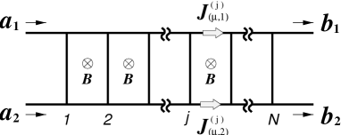
FIG. 1.: Chiral Ladder Model.

We assume that the ladder has one-dimensional legs each of which has one channel. We introduce the scattering matrix $T^{\scriptscriptstyle(j)}$ which connects the current amplitude to the left of the $j$-th rung to the current amplitude to the left of the $j\!+\!1$-th rung. The dependence of the scattering matrix $T^{\scriptscriptstyle(j)}$ on the vector potential in the legs is

$$T^{\scriptscriptstyle(j)}=\left(\begin{array}[]{cc}t_{11}^{\scriptscriptstyle(j)}\exp\{i\phi_{1}^{\scriptscriptstyle(j)}/\phi_{0}\}&t_{12}^{\scriptscriptstyle(j)}\exp\{i\phi_{1}^{\scriptscriptstyle(j)}/\phi_{0}\}\\ t_{21}^{\scriptscriptstyle(j)}\exp\{i\phi_{2}^{\scriptscriptstyle(j)}/\phi_{0}\}&t_{22}^{\scriptscriptstyle(j)}\exp\{i\phi_{2}^{\scriptscriptstyle(j)}/\phi_{0}\}\end{array}\right)$$ (23)

where $\phi_{0}\equiv\hbar c/q$ and $\phi_{1}^{\scriptscriptstyle(j)}$ ($\phi_{2}^{\scriptscriptstyle(j)}$) is the integral of $A(x)$ over the upper (lower) leg between the $j$-th and the $j\!+\!1$-th rungs with $A(x)$ being the vector potential element in the direction of the legs at position $x$. Here the matrix $t^{\scriptscriptstyle(j)}\equiv(t_{ll^{\prime}}^{\scriptscriptstyle(j)})$ is the corresponding scattering matrix in the case that the vector potential in the legs is zero. In this model the scattering matrix $T^{\scriptscriptstyle(j)}$ is the same as the corresponding transfer matrix, so the scattering matrix ${\cal{S}}^{\scriptscriptstyle(j)}\equiv({\cal{S}}_{ll^{\prime}}^{\scriptscriptstyle(j)})$ of the sub-system consisting of the first $j$ number of rungs is given by $T^{\scriptscriptstyle(j)}T^{\scriptscriptstyle(j-1)}\cdots T^{\scriptscriptstyle(1)}$.

We consider the injected current density $J_{\scriptscriptstyle(\mu,1)}^{\scriptscriptstyle(j)}$ ($J_{\scriptscriptstyle(\mu,2)}^{\scriptscriptstyle(j)}$) in the upper (lower) leg between the $j$-th and the $j\!+\!1$-th rungs, which is caused by the incident current $\mbox{\boldmath$a$}_{\mu}$ shown in Fig. 1. This current is represented as $J_{\scriptscriptstyle(\mu,\nu)}^{\scriptscriptstyle(j)}=q\rho_{0}v|{\cal{S}}_{\nu\mu}^{\scriptscriptstyle(j)}|^{2}$ where $v$ is the particle velocity in the upper (or lower) leg and $\rho_{0}$ is the local density of states $1/(2\pi\hbar|v|)$ in the one-dimensional perfect wire.

Now we connect the scattering matrix ${\cal{S}}^{\scriptscriptstyle(N)}$ of the system consisting of $N$ number of the rungs ($N\!>\!1$) to the injected current density $J_{\scriptscriptstyle(\mu,\nu)}^{\scriptscriptstyle(j)}$. Noting unitarity of the matrices $T^{\scriptscriptstyle(j^{\prime})}$, ${\scriptstyle j^{\prime}=N,N-1,\cdots,l+1}$ and using the relation $\delta\phi_{\nu}^{\scriptscriptstyle(j)}/\delta A(x_{\nu^{\prime}}^{\scriptscriptstyle(j^{\prime})})=\delta_{jj^{\prime}}\delta_{\nu\nu^{\prime}}$, where $x=x_{1}^{\scriptscriptstyle(j)}$ ($x_{2}^{\scriptscriptstyle(j)}$) is a point in the upper (lower) leg between the $j$-th and the $j\!+\!1$-th rungs, we obtain $(1/(2\pi i))\sum_{l=1}^{2}{\cal{S}}_{l\mu}^{\scriptscriptstyle(N)\dagger}\cdot\delta{\cal{S}}_{l\mu}^{\scriptscriptstyle(N)}/\delta A(x_{\nu}^{\scriptscriptstyle(j)})=(1/c)J_{\scriptscriptstyle(\mu,\nu)}^{\scriptscriptstyle(j)}$, which is just the injected current density formula (1) in the time-independent Hamiltonian case.

$\langle$ Conclusion and remarks $\rangle$ In this Letter we have discussed formulas to derive the charge current density, the charge density and their quantum mechanical current density correlations from the scattering matrix in one-particle and time-dependent Hamiltonian systems. The gauge invariance requires Eq. (13) which has to be satisfied by these local quantities. Using our formulas we obtained a relation between the local density of states and the total current density produced by incident particles at an energy in time-independent Hamiltonian systems. Specifically we verified the current density formula for a chiral ladder model.

In this Letter for simplicity we considered one-particle systems only. However our technique to derive Eqs. (6) and (9) can be used to obtain some generalizations to the formulas including many-particles’ effects. For instance, we can generalize Eq. (1) to the inelastic scattering cases by dynamical scatterers with no charge. Eqs. (6) and (9) also suggest that we can derive formulas for other local physical quantities from functional derivatives of the scattering matrix with respect to other local fields. For example, if the potential $U(\mbox{\boldmath$x$},t)$ includes the term $-q\hat{\mbox{\boldmath$s$}}\cdot\mbox{\boldmath$B$}(\mbox{\boldmath$x$},t)/2$ as an interaction effect of a spin $\hat{\mbox{\boldmath$s$}}$ with a magnetic field $\mbox{\boldmath$B$}(\mbox{\boldmath$x$},t)$, then we can calculate the local expectation value of a spin component from a functional derivative of the scattering matrix with respect to the magnetic field.

As another approach to the charge current density we can use the linear response theory [22, 23]. The connection of the scattering theoretical approach to the linear response theoretical approach in the description of local quantities is left as a future problem.

$\ast\ast\ast$

I am very grateful to M. Büttiker for stimulating discussions, encouragements and a careful reading of this Letter. Especially he gave me valuable comments and suggestions relating to the injectivity formula, time-dependent Hamiltonian problems and the gauge invariance, and introduced the chiral ladder model to me.

References

• [1] C. J. Joachain: Quantum Collision Theory, North-Holland Publishing Company (1975).
• [2] R. Landauer, Philos. Mag. 21 (1970) 863.
• [3] E. N. Economou and C. M. Soukoulis, Phys. Rev. Lett. 46 (1981) 618.
• [4] D. S. Fisher and P. A. Lee, Phys. Rev. B23 (1981) 6851.
• [5] M. Büttiker, Y. Imry, R. Landauer and S. Pinhas, Phys. Rev. B31 (1985) 6207.
• [6] M. Büttiker, Phys. Rev. Lett. 57 (1986) 1761.
• [7] T. Taniguchi, Phys. Lett. A245 (1998) 279.
• [8] J. Friedel, Philos. Mag. 43 (1952) 153.
• [9] J. S. Langer and V. Ambegaokar, Phys. Rev. 121 (1961) 1090.
• [10] R. Dashen, S. -k Ma and H. J. Bernstein, Phys. Rev. 187 (1969) 345.
• [11] E. Akkermans, A. Auerbach, J. E. Avron and B. Shapiro, Phys. Rev. Lett. 66 (1991) 76.
• [12] G. B. Lesovik, Pis’ma Zh. Eksp. Teor. Fiz. 49 (1989) 513 [JETP Lett. 49 (1989) 592].
• [13] M. Büttiker, Phys. Rev. B46 (1992) 12485.
• [14] M. Büttiker, J. Phys.: Condens. Matter 5 (1993) 9361.
• [15] M. Büttiker and T. Christen, L. L. Sohn et al. (eds.), Mesoscopic Electron Transport, Kluwer Academic Publishers (1997) p259-p289.
• [16] T. Christen, Phys. Rev. B55 (1997) 7606.
• [17] T. Gramespacher and M. Büttiker Phys. Rev. B60 (1999) 2375.
• [18] C. Barnes, B. L. Johnson, and G. Kirczenow, Phys. Rev. Lett 70 (1993) 1159.
• [19] T. Taniguchi and M. Büttiker, Phys. Rev. B60 (1999) 13814.
• [20] M. Büttiker, H. Thomas and A. Pr$\hat{e}$tre, Z. Phys. B94 (1994) 133.
• [21] M. Büttiker, Phys. Rev. B32 (1985) 1846.
• [22] R. Kubo, J. Phys. Soc. Jpn 12 (1957) 570.
• [23] H. U. Baranger and A. D. Stone, Phys. Rev. B40 (1989) 8169.