eurm10 \checkfontmsam10 \pagerange1–??
Inertial effects in three dimensional spinodal decomposition of a symmetric binary fluid mixture: A lattice Boltzmann study
Abstract
The late-stage demixing following spinodal decomposition of a three-dimensional symmetric binary fluid mixture is studied numerically, using a thermodynamicaly consistent lattice Boltzmann method. We combine results from simulations with different numerical parameters to obtain a unprecendented range of length and time scales when expressed in reduced physical units. (These are the length and time units derived from fluid density, viscosity, and interfacial tension.) Using eight large () runs, the resulting composite graph of reduced domain size against reduced time covers , . Our data is consistent with the dynamical scaling hypothesis, that is a universal scaling curve. We give the first detailed statistical analysis of fluid motion, rather than just domain evolution, in simulations of this kind, and introduce scaling plots for several quantities derived from the fluid velocity and velocity gradient fields. Using the conventional definition of Reynolds number for this problem, , we attain values approaching . At (which requires ) we find clear evidence of Furukawa’s inertial scaling (), although the crossover from the viscous regime () is both broad and late (). Though it cannot be ruled out, we find no indication that is self-limiting () at late times, as recently proposed by Grant and Elder. Detailed study of the velocity fields confirm that, for our most inertial runs, the rms ratio of nonlinear to viscous terms in the Navier Stokes equation, , is of order ten, with the fluid mixture showing incipient turbulent characteristics. However, we cannot go far enough into the inertial regime to obtain a clear length separation of domain size, Taylor microscale, and Kolmogorov scale, as would be needed to test a recent ‘extended’ scaling theory of Kendon (in which is self-limiting but not). To obtain our results has required careful steering of several numerical control parameters so as to maintain adequate algorithmic stability, efficiency and isotropy, while eliminating unwanted residual diffusion. (We argue that the latter affects some studies in the literature which report for .) We analyse the various sources of error and find them just within acceptable levels (a few percent each) in most of our datasets. To bring these under significantly better control, or to go much further into the inertial regime, would require much larger computational resources and/or a breakthrough in algorithm design.
1 Introduction
Spinodal decomposition occurs when a fluid mixture of two species and , forming a single homogeneous phase at high temperature , undergoes spontaneous demixing following a sudden drop in temperature (or ‘quench’). For suitable compositions and quenches, one enters the ‘spinodal’ regime in which the initial homogeneous phase is locally unstable to small fluctuations. (Elsewhere one finds instead a nucleation and growth mechanism which is not the subject of this paper.) For compositions close to 50/50, there then arises, after an early period of interdiffusion, a bicontinuous domain structure in which patches of -rich and -rich fluid are separated by sharply defined interfaces. The sharpness depends on the temperature drop; we assume a ‘deep quench’ for which the interfacial thickness is, in practice, on a molecular rather than macroscopic scale. In this late-stage structure, the local compositions of the fluid patches correspond to those of the two bulk phases in coexistence; the interfacial tension approaches , its equilibrium value. Although locally close to equilibrium everywhere, the structure then continues to evolve so as to reduce its interfacial area. Local interfacial curvature causes stresses (equivalently, Laplace pressures) to arise, which drive fluid motion. The interface then evolves smoothly with time between isolated ‘pinchoff events’ or topological reconnections. In principle these events reintroduce molecular physics at the short scale; however it is generally assumed that pinchoff, once initiated, occurs rapidly enough not to impede the coarsening process (but see Jury et al., 1999b; Brenner et al., 1997). Likewise it is usually assumed that at late times, the presence of thermal noise in the system is irrelevant, at least for deep quenches (but see G Gonnella & Yeomans, 1999): the problem is thus one of deterministic, isothermal fluid motion coupled to a moving interface. Precise details of the random initial condition, which is inherited from the earlier diffusive stage, are also thought to be unimportant (assuming that no long-range correlations are initially present).
For simplicity we address in this paper only the maximally symmetric case of two incompressible fluids with identical physical properties (shear viscosity , density ), and also equal volume fractions, that have undergone a deep quench. With the assumptions made above, all such fluid mixtures should, in the late stages, behave in a similar manner. More precisely, the dynamical scaling hypothesis is that, if one defines units of length and of time by
| (1) |
(which are the only such units derivable from ) then at late times any characteristic structural length should evolve with time according to
| (2) |
where is the same function for all such fluids. (A specific choice of definition for is made later on, in terms of the mean domain size.) Integrating this once gives a universal late-stage scaling
| (3) |
where we introduce ‘reduced physical units’,
| (4) |
Here an offset that is nonuniversal: it depends on the initial condition as fixed by the early stage diffusion processes. (Note that in this paper, the symbol is reserved for the reduced physical time; unscaled time is denoted , and temperature . An overdot means time derivative in whatever units are being used.)
The form of has been discussed by several authors, notably Siggia (1979) and Furukawa (1985). Siggia argued that, for , the interfacial forces induce a creeping flow of the fluid; simple force balance in the Navier–Stokes equation then gives in this, the ‘viscous hydrodynamic’ regime. Note that, in a creeping flow, the fluid velocity depends only on the instantaneous structure of the interface. (This is why the nonuniversal offset is in and not .) At later times, the force balance was argued by Furukawa to entail viscous and inertial effects; balancing these gives for , the ‘inertial hydrodynamic’ regime. It has recently been shown by Kendon (2000) that Furukawa’s assumption of a single characteristic length (for velocity gradients as well as interfacial structure) is inconsistent with energy conservation; her more detailed analysis nonetheless recovers for the domain size. Kendon’s arguments, with those of Siggia and Furukawa, are discussed in § 4, 5.
For a general review of late-stage spinodal decomposition and other aspects of phase separation kinetics, see that of Bray (1994). The problem is clearly intractable analytically: it involves a moving boundary with a complicated and non-constant topology whose initial condition is defined, implicitly, by the preceding, early-time diffusion. These features render it equally intractable to many numerical algorithms that might perform well for other fluid mechanics problems. Indeed, symmetrical spinodal decomposition has become a benchmark for various so-called ‘mesoscale’ simulation techniques, developed to address the statistical dynamics of fluids with microstructure. The results from different techniques can be compared, not only with each other and with experiment (with the caveat that one cannot realize exact symmetry between fluids in the laboratory), but with the predictions of the various scaling theories already mentioned.
In the present work, we study in detail the physics of spinodal decomposition for a symmetrical binary fluid using the Lattice Boltzmann (LB) technique (Higuera et al., 1989), in a thermodynamically consistent form pioneered by the group of Yeomans (see Swift et al., 1996). Our work, of which a preliminary report appeared in Kendon et al. (1999), advances significantly the state of the art for simulations of spinodal decomposition, and for LB simulations of fluid mixtures. In any such simulation, a balance must be struck between discretization error at small scales, and finite size errors (arising in our case from periodic boundary conditions) at large ones; this compromise is quite subtle, as we discuss below. It means that any individual simulation run can produce only around one decade of data for the curve. This is true for all first-principles simulation methods: in three dimensions there cannot be more than two decades, or at most three, separating the discretization length from the system size, before deduction of a half-decade safety margin at each end. (Three decades before such deduction is optimistic; it means simulating at least degrees of freedom.)
Despite this restriction, by careful scaling and combination of separate datasets for eight large () simulation runs, we are able to access an unprecedented range of and (five and seven decades respectively) including regions of the curve not studied previously. We find nothing to contradict the universality of Equation (3), but nor can we completely rule out violations of it. We gain the first unambiguous evidence for a regime in which inertial effects dominate over viscous ones, and find clear evidence for scaling in this regime. In this and other regions of the curve, we study the statistics, not only of the interfacial structure, but also of the fluid velocity. (The latter was not addressed in detail by previous simulations.) On entering the inertial hydrodynamic regime we find some evidence for breakdown of simple scaling of velocity gradients, as proposed by Kendon (2000), but our data does not extend far enough into this regime to offer a meaningful test of her alternative proposals.
To obtain our new results, we have had to push the LB technique to its limits. For statistics based on the domain size, errors at the level of several percent, arising from each of several different sources (residual diffusion, lattice anisotropy etc.) remain. We do make a systematic attempt to identify and minimize the various sources of errors – a somewhat arduous task that, our work suggests, has been neglected in several previous studies. The errors for some of our velocity statistics (especially those for spatial derivatives of the velocity) are much larger. Nonetheless we present the data, such as it is, because it highlights several issues both in the physics of spinodal decomposition and in how simulation results should be obtained, analysed and interpreted.
The rest of this paper is organized as follows. § 2 outlines the thermodynamics of the binary fluid system, and § 3 its governing equations. § 4 and § 5 outline the simple and extended scaling analyses referred to above. § 6 describes the LB method in the form that we use; § 7 describes how the simulation parameters are chosen. § 8 outlines a number of validation tests. § 9 gives our results for the evolution of the interfacial structure, § 10 those for the velocity field and § 11 those for the velocity derivatives and related quantities. § 12 summarizes our conclusions. Two appendices give further information on the effects of residual fluid compressibility in the LB method and on the relation between our work and that of previous authors.
2 Thermodynamics
Although we are interested in the late-stage demixing of two isothermal, incompressible fluids separated by sharp interfaces, the LB method resorts to a more fundamental approach, in which these interfaces are described as excitations of a thermodynamic field theory. The central object is the Helmholtz free energy
| (5) |
where is the internal energy, the temperature and the entropy of the system.
In a system at fixed volume , and fixed contents and temperature, equilibrium states are given by global minima of the free energy, . For a symmetric fluid mixture, is a functional of a single composition variable , defined as where the ’s are number densities, and of the mean fluid density . (We take unit mass for and particles without loss of generality.) In the incompressible case, is fixed; we leave it as a parameter in what follows. Further restricting attention to homogenous states (so that is the same everywhere), we can write
| (6) |
Within mean-field theories of fluid demixing, one predicts that has everywhere positive curvature at high temperatures, but becomes concave below a critical temperature . The resulting curve is as shown in Figure 1, with symmetric minima at . Below , the free energy is therefore minimized by creating two bulk domains (of equal volume) at compositions instead of a single homogenous phase with (which is our presumed initial condition). The same phase separation occurs for any other between , but in this case the domain volumes are unequal; for sufficient asymmetry this causes depercolation. (In a depercolated, droplet structure, coarsening can only occur by diffusion so that the scaling arguments given above cease to apply. We do not address this here.)

The resulting phase diagram is shown in Figure 2. Spinodal decomposition occurs for any quench that leaves the system beneath the spinodal line, on which changes sign. Immediately after such a quench, the system is locally unstable: the free energy can be lowered, in any local neighbourhood, by creating two domains whose composition differs only infinitesimally from the initial one. (The resulting free energy density lies on a line connecting two points on at the new compositions; in the convex region, this causes a reduction in .) Accordingly, infinitesimal fluctuations will grow by diffusion until there is local coexistence of domains at compositions approaching .

To describe quantitatively both the domains and the interfaces between them, one must specify not just but the free energy functional, . An acceptable choice is the square gradient model (see Bray, 1994)
| (7) |
where is as shown in Figure 1, and the term in penalizes sharp gradients in composition. This ensures smooth local deviations from near the interface, and provides a nonzero interfacial tension which can be calculated as follows. We consider a flat interface between two domains, introducing a coordinate normal to it, . Stationarity of requires
| (8) |
Integrating this once across the interface and setting , at its centre gives
| (9) |
The excess free energy per unit area of interface is then given by
| (10) |
By exploiting the fact that in the bulk fluid, and using Equation (9), we obtain
| (11) |
Given a form for the potential, , a value for the interfacial tension can thus be calculated. This is done for the model used in our simulations in § 6.
We now turn to the (exchange) chemical potential, , which describes the change in for a small local change in composition:
| (12) |
Within the LB approach, the coupling between interfacial and fluid motion arises as follows. In the presence of a nonuniform composition, there is a thermodynamic force density acting at each point on the fluid. (The two species are pulled in opposite directions by the chemical potential gradient; the net force vanishes only if .) This force density can also be written as the divergence of a ‘chemical’ pressure tensor:
| (13) |
where it is a straightforward exercise to confirm that
| (14) |
Note that only the last term is anisotropic; the rest contributes, in effect, to the isotropic fluid pressure . By integrating (13) across an interface, and using Eq. (14), one finds that there is, in static equilibrium, a finite pressure difference across a curved interface, called the Laplace pressure:
| (15) |
where is the interfacial curvature.
Throughout the above, our description in terms of a smooth composition variable , usually known as the order parameter, assumes a coarse-graining so that the smallest length scale under consideration is larger than the average distance between molecules. In equilibrium, this coarse-graining is an almost trivial operation, but for the dynamical description desired below, certain conditions must be met. On scales smaller than the coarse-graining length, the system must remain in local equilibrium, while the variations of interest at larger scales must be slow on the scale of the time it takes for that local equilibrium to be reached.
This does not mean that the microscopic scales can be forgotten from here on. Although usually a macroscopic description is sufficient to fully understand the system, ultimately it is still the microscopic interactions that are driving the system and determining the dynamics. In particular, any interface between the two fluids will have a microscopic size and structure. It is always a possibility that the microscopic behaviour can intrude at the macroscopic level (for example, by interfering with pinchoff) and change the results predicted by any simple macroscopic considerations. In particular, when using numerical models, care must be taken that the microscopic behaviour in these models is admissible.
3 Governing Equations
The equation of motion for is taken to be a convective diffusion equation of Cahn Hilliard type (see Bray, 1994; Swift et al., 1996)
| (16) |
where is an order-parameter mobility (here assumed independent of ) that controls the strength of the diffusion, and is the fluid velocity. This equation states that the order parameter responds to composition gradients by diffusion (the term), and also changes with time because it is advected by the fluid flow (the term).
The fluid velocity in turn obeys the Navier–Stokes equation (NSE), which for an incompressible fluid reads
| (17) |
Here is the ‘thermodynamic’ (or conservative) part of the pressure tensor, and contains two pieces: an isotropic contribution , chosen to maintain constant , and the ‘chemical’ pressure tensor, , defined previously in (14). Recall that by (13), the chemical term can equally well be represented as a body force density acting on the fluid, so that Eq. (17) also reads
| (18) |
4 Simple Scaling Analyses
The pair of coupled nonlinear differential equations, (16) and (17), are intractable, but various dimensional and scaling ideas may be used to find out how fast the domains grow once the diffusive period is over. All these analyses assume that the interface can be characterized by a single length scale — that is, it is basically smooth, with radii of curvature that scale as the domain size itself, which is much larger than the interfacial thickness.
Many domain-scale length measures are possible; we use , the inverse of the first moment of the spherically averaged structure factor, :
| (19) |
where is the modulus of the wave vector in Fourier space, and
| (20) |
with the spatial Fourier transform of the order parameter. The angle brackets denote an average over a shell in space at fixed .
The aim of scaling analyses is to find the form of the time dependence of by considering the NSE (18), and balancing the force from the interface,, against the viscous and inertial terms which tend to oppose its motion. The interfacial force density, , can be approximated as follows. The curvature, , is of order , since is roughly the size of the domains. This sets the scale of through (15), as . Likewise the gradient operator, , can be approximated by in Equation (14), which then reads
| (21) |
Now we turn to the remaining terms in the NSE (18). We start by assuming that the length also controls the magnitude of as far as velocity gradients are concerned. Approximating also the fluid velocity, , by the velocity of the interface , gives for the viscous and inertial terms respectively
| (22) | |||||
| (23) |
Under conditions in which the inertial terms are negligible, the force from the interface will be balanced by the viscous force, giving . Integrating this gives,
| (24) |
Thus the domain size is predicted to grow linearly with time in the region where the fluid flow is viscous dominated. This is the result of Siggia (1979). Linear growth has been reported in experiments by, for example, Kubota et al. (1992); Chen et al. (1993); Hashimoto et al. (1994), and in simulations incorporating hydrodynamics by Koga & Kawasaki (1991); Puri & Dünweg (1992); Alexander et al. (1993); Laradji et al. (1996); Bastea & Lebowitz (1997) and Jury et al. (1999b).
To find the growth rate in the inertial region, Furukawa (1985) balanced instead the inertial and interfacial terms; assuming again only one relevant length, he obtained
| (25) |
Integrating this twice gives, for large enough , , so that the domain size grows as . This result has not yet been observed experimentally (for reasons we discuss later, § 12). There are a few previous claims to see this in simulation (Ma et al., 1992; Appert et al., 1995; Lookman et al., 1996), but none reliably establish dominance of inertial over viscous forces as we do below in § 10.
Comparing the results of (24) and (25) allows us to estimate a characteristic domain size, , and characteristic time, at which the crossover from viscous to inertial scaling occurs. (To be precise, we can define by the interception of asymptotes on a log-log plot.) This leads to , with defined in 1. Converting to reduced physical units , as defined previously, and invoking the dynamical scaling hypothesis, we have respectively
| (26) |
where and are dimensionless numbers that should be universal to all incompressible, fully symmetric, deep quenched fluid mixtures. What scaling theories cannot predict, of course, are values of the universal constants , other than to state that these are ‘of order unity’.
In fact our simulations show that is between and , which is ‘of order unity’ only in a rather unhelpful sense; the implications of this are discussed in § 12 below. We will also find that the crossover region, between the asymptotes described by (26), is several decades wide. Although there is no explicit scaling prediction for the behaviour within this crossover region, its width means that each individual simulation dataset, either within or outside the crossover, can be well-described by a single scaling exponent, , such that
| (27) |
where , and . We use this form below, when analysing our numerical data.
5 Extended Scaling Analysis
In what follows we will find it useful to compare directly the relative magnitude of the various terms in the NSE. Two ratios have therefore been defined, the rms ratio between the acceleration term and the viscous term,
| (28) |
and the rms ratio between the nonlinear term and the viscous term,
| (29) |
Here denote spatial averages (though an ensemble average might be preferable under some conditions). These ratios obey where the inertial terms dominate and where the viscous term dominates. The ratio we identify as the ‘true’ Reynolds number, that is, a dimensionless measure of the relative importance of nonlinearity in the NSE.
When , (29), is simplified using the normal scaling assumption (), the result is the following estimate:
| (30) |
Assuming that the characteristic velocity scale is , one finds (following Furukawa, 1985; Grant & Elder, 1999) the Reynolds number estimate ,
| (31) |
This ‘order-parameter Reynolds number’ has the advantage, in simulations, that it is computable from without direct access to any fluid velocity statistics. However, is only a good estimate of the true Reynolds number , if the simple scaling for velocity gradients of does indeed hold. This assumption leads to the following paradox, as noted by Grant & Elder (1999). According to (31), if in the inertial region , then which becomes indefinitely large as time proceeds. Grant and Elder argued that this could not be physical, on the grounds that an infinite Reynolds number would imply turbulent remixing of domains: this would limit the domain growth to such a speed that remained bounded at late times. (31) then demands a lower asymptotic growth exponent, , as .
However, a closer look at the scaling of all the terms in the NSE admits an alternative resolution. Kendon (2000) pointed out that a minimally acceptable scaling theory should allow, not only force balance in NSE, but a balance of terms in the global energy equation, which for an isothermal, incompressible fluid reads
| (32) |
where is the dissipation rate, and is the rate of energy transfer from the interface to the fluid. Retaining the assumption that the interface (as opposed to the velocity field) has just one characteristic length, is readily estimated from (21) as .
Applying the simple scaling for velocity gradients () to each term in (32) gives the following energy ‘balance’ in the inertial regime where :
| (33) |
where factors of are retained to aid identification of the terms. At first sight this suggests a balance of interfacial and inertial terms, with the viscous contribution negligible, at late times: this is Furukawa’s assumption. However, the signs show this to be inconsistent: the kinetic energy and the energy stored in the interface are both decreasing with time, so these cannot properly be balanced against each other.
This exposes a central defect of the simple scaling analysis in the inertial regime. It is well known, of course, that even the simplest theories of fluid turbulence entail several length scales (whereas more modern ‘multiscaling’ theories have, in effect, infinitely many, Frisch, 1995). In the simplest, Kolmogorov-type approach (see Frisch, 1995; Kolmogorov, 1941), the important lengths are the Taylor microscale111 The prefactors in the definitions of the Taylor and Kolmogorov microscales differ between sources.
| (34) |
characteristic of velocity gradients, and the Kolmogorov (dissipation) microscale,
| (35) |
the length scale below which nothing interesting occurs. (Energy is dissipated at or above the scale .)
Kendon (2000) argued that in a binary fluid system where the fluid motion has become turbulent, the velocity follows the interface and scales as , but the first and second gradients of velocity have scalings set by and respectively, rather than by . Within this simplified (Kolmogorov-level) description, the only scalings for these three lengths found physically admissible by Kendon for the inertial regime were . In the NSE, this gives for the acceleration, convection, viscous and driving terms the following scalings:
| (36) |
The predicted outcome is thus a balance between the nonlinear and dissipative forces that is decoupled from the interfacial motion, while interfacial stresses balance fluid acceleration. The existence of a nonlinear/viscous balance implies an asymptotically finite value for the ratio of the corresponding terms in NSE, that is, a finite asymptote for the true Reynolds number . On the other hand, since the result for the domain scale, , survives unaltered from the simple scaling theory, the Reynolds number estimated from the order parameter, , continues to grow indefinitely. This suggestion, although speculative, appears to resolve the issue raised by Grant and Elder, without requiring a change in the domain scale growth law (nor any breakdown of universality of (3)).
To summarise, Kendon (2000) predicts a balance in which energy is first transferred from the interface () to large scale fluid motion (). The nonlinear term () then transfers the energy from the large scales down to smaller scales where dissipative forces () finally remove it from the system. The resulting energy cascade thereby decouples the energy input scales from the dissipation scales — a familiar enough idea in turbulence theory (Kolmogorov, 1941). In contrast, in the viscous hydrodynamic regime, the simple (one-length) scaling theory is already consistent with energy conservation, and all its results are recovered. Kendon’s predictions for scaling are summarised for ease of reference in table 1.
| Quantity | viscous | inertial region | ||||
|---|---|---|---|---|---|---|
| region | simple | new | ||||
| scaling | scaling | |||||
| 1 | 2 | /3 | 2 | /3 | ||
| 1 | 2 | /3 | 1 | /2 | ||
| 1 | /2 | 1 | /2 | 5 | /12 | |
| 0 | 1 | /3 | 1 | /3 | ||
| 4 | /3 | 4 | /3 | |||
| , | 4 | /3 | 7 | /6 | ||
| 2 | 5 | /3 | 7 | /6 | ||
| 2 | 4 | /3 | 4 | /3 | ||
| 1 | 1 | /3 | 1 | /3 | ||
| 1 | /3 | 1 | /6 | |||
| 1 | /3 | 0 | ||||
| 2 | 2 | 5 | /3 | |||
6 Numerical method
The model system described by (16) and (17) was simulated numerically using a modular LB code called Ludwig, described in detail in Desplat, Pagonabarraga & Bladon (2000a). It has both serial and parallel versions; the parallel code uses domain decomposition and the MPI (message passing interface) platform. Any cubic lattice can be used with the Ludwig code; the lattice parameter is taken as unity, as is the timestep , thereby defining ‘simulation units’ of length and time.
Here we chose the D3Q15 lattice, a simple cubic arrangement in which each site communicates with its six nearest and eight third-nearest neighbours. The fluid dynamics is, as usual (see Higuera et al., 1989; Ladd, 1994) encoded at each site by a distribution function , where the subscript obeys . This ascribes weights to each of 15 velocities : one null, six of magnitude , eight of magnitude , with directions such that each velocity vector points toward a linked site. In order to model the binary fluid, a second set of distribution functions, , is also used, following Swift et al. (1996). The ’s are defined such that
| (37) |
where the sum is over all directions, , at a single lattice point, while for the same sum gives the order parameter,
| (38) |
(At this point, our algorithm departs from that of Swift et al. (1996), who would have on the right. The two methods differ only by terms that vanish in the incompressible limit of interest, where everywhere.)
The momentum, (with a cartesian index) is then given by
| (39) |
where . The full pressure tensor, , is given by
| (40) |
This expression includes not only the conservative stress but also dissipative (viscous) contributions, and a trivial ‘kinetic pressure’ which arises in any fluid moving at constant velocity .
The distribution functions obey discrete evolution equations involving simple first-order relaxation kinetics toward a pair of equilibrium distributions:
| (41) |
| (42) |
thus defining two relaxation parameters . In our use of the code we select which causes to be reset to each time step. The viscosity is determined by , with in lattice units. The equilibrium distributions, and , can be derived from (37) – (39), along with the condition that the order parameter is advected by the fluid,
| (43) |
and that the pressure tensor and chemical potential at equilibrium obey
| (44) | |||||
| (45) |
The parameter controls the order parameter mobility via , so that in our case. (Note that in Kendon et al. (1999) and Cates et al. (1999), the quoted values of are in fact values and should therefore be halved to give the true order parameter mobility.) The second term on the right in (44) is the trivial ‘kinetic pressure’, with an analagous term in Eq.(45).
By expanding to second order in velocities and solving for the coefficients one obtains
| (46) |
Here, is an index that denotes the speed, 0, 1, or , and , and are constants given by
| (47) |
| (48) |
| (49) |
The equilibrium distribution for the order parameter, , is the same as for , with th replaced by in the above equations. The above results follow Swift et al. (1996), generalised to three dimensions.
To complete the model specification, one must introduce expressions for the pressure tensor and chemical potential derived from the free energy functional. In this study we chose in (7) a simple ‘’ model for :
| (50) |
where . (The term in is discussed below.) With this choice one finds , and using (11), (12),
| (51) | |||||
| (52) |
The equilibrium interfacial profile in given by , where is the normal coordinate introduced previously, and
| (53) |
is a measure of the interfacial width.
An important addition to (50) is the term dependent on density , here chosen as an ‘ideal gas’ type contribution (up to the factor 1/3). This gives a diagonal term in the thermodynamic pressure tensor, which becomes
| (54) |
so that the thermodynamic stress obeys . Thus in practice , which is the isotropic pressure contribution normally viewed as a Lagrange multiplier for incompressibility. But in fact, our LB algorithm does not know that the fluids are meant to be incompressible; instead the ideal-gas term is relied upon to enforce incompressibility to within acceptable numerical tolerances. (This avoids a separate calculation, at each time step, of the fluid pressure and renders the algorithm local.) Compressibility errors can be minimized by increasing the coefficient of in (50), which would require a shortened time step, or for fixed time step, by reducing the magnitudes of , and together so that an acceptable level of incompressibility is maintained. The second route is followed here.
The chosen functional, (50), has a number of points in its favour for numerical simulation. The main terms in and are simple powers of , so are easy and quick to evaluate. (Models involving logarithms or trigonometric functions (Swift et al., 1996) pay a heavy price in computational efficiency.) Further, the shape of the “” potential is fairly smooth, avoiding very steep gradients that might lead to inaccuracy and instability when approximated numerically on a lattice. We nonetheless need to evaluate spatial gradients of ; this is done using all 26 (first, second and third) nearest neighbours on the D3Q15 lattice, so that numerically
| (55) |
| (56) |
Note that these are not the only possible choices and that others will only coincide when all gradients are small on the scale of the lattice. There may be considerable scope for improvement by optimising the choices made, but we leave this for future work.
As usual in LB, we have chosen a lattice with enough symmetry to ensure that the rotational invariance of the fluid mechanics is faithfully represented (Higuera et al., 1989). However, this does not guarantee that the same holds for the thermodyamic properties. With our choice of free energy functional, (50) and the above gradient discretisation, rotational invariance in the thermodynamic sector is recovered only when all order parameter gradients are weak, which in principle requires . In practice, a compromise is necessary; we return to this in § 8.2 below.
Finally, the hydrodynamic behaviour of the LB technique requires detailed comment. The hydrodynamic equations that correspond to LB can be obtained by making a Chapman-Enskog expansion of the Boltzmann equations (41,42). If we consider the expansion for the distribution function (which relates to the fluid momentum) we arrive at
| (57) | |||||
where and are the shear and second viscosities, respectively. For our single-relaxation LB scheme .
The first line of Equation 57 corresponds to the standard Navier Stokes equation, and shows that, through these terms, the model recovers both the compressible and incompressible features of isothermal hydrodynamics. 222Note that when modeling a macroscopic length, , the ratio will be larger than in typical real fluids; due to the presence of the lattice, LB does not have a sharp separation between the compressible and incompressible time scales. In this respect, it resembles a high viscosity fluid, Hagen et al. (1997).
The second line in Equation 57 contains spurious terms, which arise partly because the enthalpic interactions that lead to the non-ideal behaviour of the LB fluid (or fluid mixture) are introduced through equilibrium information only. (In a Hamiltonian system, the same interactions that perturb the equilibrium state away from an ideal gas would also be responsible for the dynamics.) Of the two terms, the second one is not Galilean invariant but is cubic in the velocity. It will be negligible for small velocities (recall that the LB algorithm anyway requires fluid velocities that are small in lattice units). The first term can be decomposed into a Galilean-invariant part, which is a product of gradients of the pressure and velocity, and a non-Galilean invariant contribution. The product term is small compared to the Navier-Stokes terms, which are linear in such gradients, whenever these are weak; the non-Galilean invariant term is small under the same conditions. There have been recent proposals to enforce Galilean invariance within compressible multiphase lattice-Boltzmann schemes, Holdych et al. (1998), and this is a desirable feature of future algorithms. Nonetheless, under circumstances where all hydrodynamic fields vary smoothly on the lattice scale, the spurious terms appearing in the second line of (57) will typically be smaller than the retained ones of the NSE equation in the first line.
The evolution equation for the order parameter can be obtained analogously, by performing a gradient expansion of the linearized Boltzmann equation (42). This leads to
| (58) |
Equation (58) has the usual form of a convection-diffusion equation, so long as one chooses as a constant, except for the last term. As with (57), this Galilean-invariant term arises as a result of the way in which the non-ideality of the fluid mixture is introduced; like the first spurious term in (57) it contains one higher derivative than the term that enters the Navier Stokes equation, and is expected to be small for similar reasons. In Appendix A we confirm explicitly that, in the incompressible limit only, this spurious term does not modify the hydrodynamic modes of a binary mixture, at the level of a linearised expansion about a uniform quiescent fluid.
In summary, for a nominally incompressible fluid the correct fluid behaviour is recovered in the only regime where it can justifiably be expected, namely, when all the hydrodynamic fields vary slowly on the lattice length scale. Within the current LB algorithm, one also depends on having only slight fluid compressibility: this eliminates a spurious coupling between order parameter and momentum fluxes (Appendix A, and Swift et al., 1996; Holdych et al., 1998). Because of this it is important, with the current algorithm, to monitor closely the actual fluid flow.
7 Parameter Steering
Since it is possible in a single simulation to sample only a small piece of the curve, it is necessary to work one’s way along this curve via a series of different runs. This means varying relative to the lattice constant so that an appropriate window of reduced length scales lies within the range of the simulation. Put differently, one must set, in lattice units, .
In the simulations, however, we need to choose not one parameter value () but seven (, and also ). Few of these parameters can, in practice, be set independently: an unguided choice would typically produce a simulation that either did nothing over sensible timescales or became unstable very rapidly. To avoid these outcomes, careful parameter steering is required. This was done by semi-empirical testing using small (workstation) simulation runs until satisfactory choices emerged. Runs on and lattices were used to confirm these before committing the resources for runs. The resulting parameters are summarized in tables 2 and 3. The guiding principles that emerged from this process, as well as the actual parameter values, are of some interest to those planning future work with LB. They are now summarised briefly, followed by a discussion (§ 8) of several validation exercises that were then undertaken.
In essence, our navigation of the curve involves steering three parameters () at fixed values of the remaining four (). Firstly, the (mean) density can be set to unity without loss of generality; we do this. Second, we set by choosing ; in terms of the original definition of the order parameter () this amounts to a simple rescaling of . Varying in proportion to then gives control over the interfacial tension (51) while retaining a fixed interfacial width in lattice units (Eq. (53)); this keeps thermodynamic lattice anisotropies under control (§ 8.2).
To achieve an efficient simulation, one requires the interfacial velocity to be of order in lattice units during the main part of each run. (Any slower will exhaust resources; any faster will give compressible and inaccurate fluid motion, and, in all likelihood, numerical instability.) At each point on the curve, this gives, a posteriori a relation between and . Thus to access large one clearly requires small ; but to avoid compressibility problems (§ 8.4) this must be done by reducing viscosity rather than increasing interfacial tension. Maintenance of numerical stability (§ 8.1) requires in fact that we decrease with decreasing ; however, these factors do not cancel in and a wide range of values (about six decades) can stably be achieved. Thus we were able to explore the viscous, crossover, and inertial regimes; these various regimes are delineated quantitatively in § 9.2 below.
Setting the correct mobility is crucial throughout. Across the whole curve, one has to ensure that is large enough that interfaces relax to local equilibrium on a time scale fast compared to their translational motion. But if is made too large, residual diffusion becomes a significant contributor to the coarsening rate, contaminating the data. This tradeoff can be eased in principle by going to larger system sizes than those currently available. It could also be improved by making a function of , setting (for example) . This would have the effect of giving strong diffusion only where it is needed, in the interfacial region. However, implementation of this within LB is not trivial (Swift et al., 1996); specifically it is not enough to make in (45) -dependent333 Since in (58) enters in the form rather than as as would be required if were not constant..
It is not surprising that mobility is a limiting factor at large (viscous regime, small ): diffusion will always enter if the fluid flow is slow enough (high enough ). But mobility factors also come into play at the inertial end (small , large ): in physical units, the interface in this regime is unnaturally wide and to maintain it in diffusive equilibrium (and keep the algorithm stable) again requires relatively large . These cause residual diffusion which, for our system sizes, limits from above the range of accessible.
Finally, we found that accuracy in the viscous regime (small , large ) is compromised when the viscosity becomes too large (of order unity, in lattice units). The signature of this is an apparent breakdown of energy conservation (see § 11.5). We are not sure of its origins, but note that too large a viscosity causes the dynamics of momentum diffusion and that of sound propagation (density equilibration) to mix locally. In an almost steady flows this should not matter, but in the small regime the viscous and interfacial terms in NSE are both numerically large. In principle these balance to give negligible fluid acceleration but their numerical cancellation may be imperfect. Although any such local accelerations are numerical in origin, the response to them may need to be accurate, if the global physics is to be handled correctly. We speculate that this is a limiting factor in our exploration of the curve at the lower end.
In this study, the largest system size was , although due to disk storage limitations, the results from this system size were analysed only after coarse-graining down to . The coarse-graining was done by averaging over blocks of eight neighbouring lattice sites to create one coarse-grained value. Runs at and were also done, and results for all calculated quantities were compared between and runs with the same parameters, to identify any effects of coarse-graining. The main and simulations were run respectively on the EPCC Hitachi SR-2201 machine (4 processors) and the EPCC Cray T3D (64 and 256 processors). Follow-up studies used in some of the velocity analysis work, and for additional visualisation, were made on the CSAR Cray T3E at Manchester.
Typical runs required, in the case, around 3000 T3D processor hours CPU, and time steps to reach the point where finite size effects set in (see § 8.5). All simulation were run with periodic boundary conditions; the initial configuration was always a completely mixed state, with small random fluctuations. For each run, the order parameter, , and the fluid velocity vector at each lattice site were saved periodically for later analysis. The sampling frequency was limited by the available disk space. Typically, data was saved every 300 time steps giving, over a run of time steps, around 4Gb of data.
| Run | ||||||||||||||
|---|---|---|---|---|---|---|---|---|---|---|---|---|---|---|
| Run028 | 36 | 935 | 0 | .083 | 0 | .053 | 1 | .41 | 0 | .1 | 0 | .055 | ||
| Run022 | 5 | .95 | 71 | 0 | .0625 | 0 | .04 | 0 | .5 | 0 | .5 | 0 | .042 | |
| Run033 | 5 | .95 | 71 | 0 | .0625 | 0 | .04 | 0 | .5 | 0 | .2 | 0 | .042 | |
| Run029 | 0 | .952 | 4 | .54 | 0 | .0625 | 0 | .04 | 0 | .2 | 0 | .3 | 0 | .042 |
| Run020 | 0 | .15 | 0 | .885 | 0 | .00625 | 0 | .004 | 0 | .025 | 4 | .0 | 0 | .0042 |
| Run030 | 0 | .01 | 0 | .016 | 0 | .00625 | 0 | .004 | 0 | .0065 | 2 | .5 | 0 | .0042 |
| Run019 | 0 | .00095 | 0 | .00064 | 0 | .00313 | 0 | .002 | 0 | .0014 | 8 | .0 | 0 | .0021 |
| Run032 | 0 | .0003 | 0 | .00019 | 0 | .00125 | 0 | .0008 | 0 | .0005 | 10 | .0 | 0 | .00083 |
| Run | ||||||||||||||
|---|---|---|---|---|---|---|---|---|---|---|---|---|---|---|
| Run010 | 381 | 25656 | 0 | .125 | 0 | .08 | 5 | .71 | 0 | .5 | 0 | .084 | ||
| Run026 | 36 | 935 | 0 | .083 | 0 | .053 | 1 | .41 | 0 | .25 | 0 | .055 | ||
| Run027 | 36 | 935 | 0 | .083 | 0 | .053 | 1 | .41 | 0 | .1 | 0 | .055 | ||
| Run014 | 5 | .95 | 71 | 0 | .0625 | 0 | .04 | 0 | .5 | 0 | .5 | 0 | .042 | |
| Run008 | 0 | .952 | 4 | .54 | 0 | .0625 | 0 | .04 | 0 | .2 | 0 | .5 | 0 | .042 |
| Run018 | 0 | .15 | 0 | .885 | 0 | .00625 | 0 | .004 | 0 | .025 | 4 | .0 | 0 | .0042 |
| Run015 | 0 | .00095 | 0 | .00064 | 0 | .00313 | 0 | .002 | 0 | .0014 | 8 | .0 | 0 | .0021 |
| Run031 | 0 | .0003 | 0 | .00019 | 0 | .00125 | 0 | .0008 | 0 | .0005 | 10 | .0 | 0 | .00083 |
8 Validation and Error Estimates
8.1 Numerical stability
The LB method is not generally stable. In fact, our experience suggests that, whatever parameters are chosen, any run would eventually become unstable if continued for long enough; this is not dissimilar to some molecular dynamics algorithms, Allen & Tildesley (1987). During testing, a reliable picture was acquired of the characteristic way in which this happens. When the inaccuracies have built up to the point of failure, the velocities become very large over a small number of time steps until numerical overflow causes the code to stop running. There seems to be no danger of taking data from a period when the system might be far from accurate but still apparently running successfully, since the onset is so rapid. Thus there are several runs among the set used for final data analysis where the run ended prematurely due to instabilities, but the data prior to the instability has been considered sufficiently reliable to be used.
8.2 Anisotropy and interfacial tension
The elimination of lattice anisotropy in the thermodynamic sector of the model requires in lattice units, to ensure that the interfacial tension is independent of interface orientation. In practice this goal must be balanced against other demands. To test the extent of the problem, a spherical droplet (radius 32 lattice units) of fluid B surrounded by fluid A was allowed to equilibrate. The interface profile was then measured by evaluating the mean and standard deviation of the order parameter at various radii (binned on the scale of 0.1 lattice units) from the droplet centre. The result is presented in figure 3 for and for . Note that the ‘width’ of the interface, as judged by eye, is actually about .

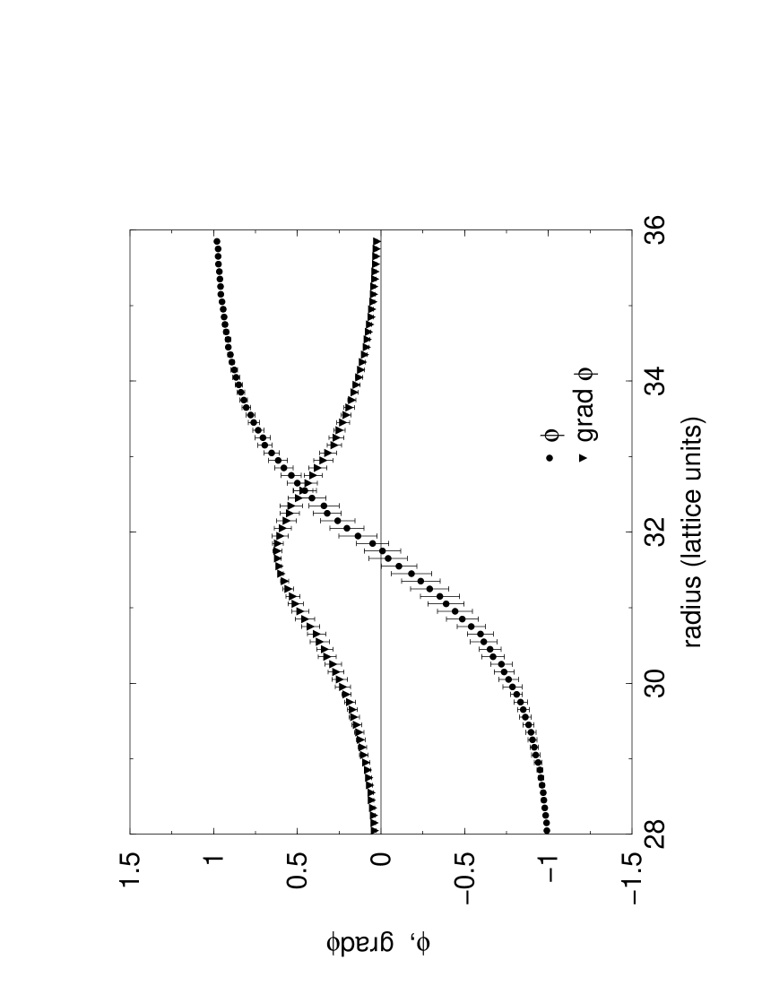
A closer look at the droplet shape (not shown) in each case reveals that the sphere has deformed slightly by squeezing along the Cartesian lattice directions and expanding along the diagonals. This deformation is about 3.5% for the narrower profile and about 1.5% for the wider profile. A similar test, done with a sphere of radius , confirmed that this deformation was not due to any tendency of the interface to lock onto specific lattice sites but purely from anisotropy of the tension.
If all else were equal, the wider interface would be chosen. However, the computational penalty for wider interfaces is severe. To maintain these in local equilibrium, the mobility must be high enough to allow diffusion across several on a timescale faster than fluid motion. For the wider interface () the resulting residual diffusion then contaminates much of the remaining range. It was thus found necessary to sacrifice some isotropy for efficiency, and the narrower profile with was used for the main runs in this work. The resulting anisotropies are marginally detectable by eye in visualisations of the interface for the spinodal system (e.g. figure 10 below). We estimate that they contribute systematic errors of a few percent to the growth rate , which is comparable to other sources of error.
The mean interfacial tension was measured for each parameter set by allowing an interface to come to equilibrium and numerically performing the integration in (11). Both terms were evaluated, and an average taken over various configurations. This gives values for the interfacial tension, shown in table 4, that are systematically about 10–15% smaller than the theoretical values. (The statistical error is a few percent.) The difference is due to the narrow interface leading to inaccuracies in the gradient calculations. But as far as the simulation is concerned, this systematic effect is removed by our using the measured value of the interfacial tension in subsequent calculations of and .
| theory | measured | ||||||||||
|---|---|---|---|---|---|---|---|---|---|---|---|
| 0 | .083 | 0 | .053 | 1 | .41 | 0 | .1 | 0 | .063 | 0 | .055 |
| 0 | .063 | 0 | .04 | 0 | .5 | 0 | .5 | 0 | .047 | 0 | .042 |
| 0 | .0063 | 0 | .004 | 0 | .025 | 4 | .0 | 0 | .0047 | 0 | .0042 |
| 0 | .0031 | 0 | .002 | 0 | .0014 | 8 | .0 | 0 | .0024 | 0 | .0021 |
| 0 | .0013 | 0 | .0008 | 0 | .0005 | 10 | .0 | 0 | .00094 | 0 | .00083 |
8.3 Local equilibrium and residual diffusion
Errors in the intereface-driven dynamics can arise if the interface is not maintained in local equilibrium. This was tested as follows. Since the bulk fluid is fully separated (), one expects where is the area per unit volume and angle brackets are a real-space (site) average. Within a given run, any departure from constancy of the product is thus an indicator that the interfaces are failing to keep up with the evolution of the surrounding fluid. (This product could have different asymptotic values in the viscous and inertial regimes, so the product need not be the same in different runs.) At the lowest values used for the mobility (deep in the viscous regime) there was measurable deviation from constancy, from which the nonequilibrium deviations in were estimated to be of order 5%. Any deviations in the inertial regime were, however, smaller than this.
Careful checks were made to exclude residual diffusive contributions to the coarsening process. This was done using comparator runs in which the viscosity was set to an extremely large value so that coarsening was purely diffusive. (Such runs are depicted in figure 7 below.) From this, the diffusive coarsening rate was found as a function of domain size. Then for the full run (with fluid motion reinstated) all data was excluded for which this diffusive coarsening rate exceeded 2% of the full rate. This whole procedure was repeated with a limit of 1% instead of 2% on the residual diffusion. The values of the fitted exponent as per (27) (given in the last column in table 5), did not change beyond the estimated errors so the limit of 2% diffusion was taken to provide sufficient accuracy.
The result of this choice was exclusion of data with (varying somewhat between runs). Had a wider interface been used (see § 8.2) then by the same criterion would be much larger giving very little usable data.
8.4 Compressibility and small scale structure
The Ludwig code will only work correctly at low Mach number. This requires where the sound speed is in lattice units. Since in our simulations is of order 0.01, we expect our the binary fluid mixture to remain incompressible (), at least at length scales larger than a few lattice sites; in Fourier space, we expect at all but high . figure 4 shows the rms ratio of the radial to the transverse velocity components in Fourier space as a function of wavenumber, and also the spherically averaged velocity structure factor, , for various runs. Also shown for comparison is single fluid turbulence444 The single fluid turbulence simulation method sets the radial component identically to zero thus guaranteeing perfect incompressibility., generated using pseudo-spectral direct numerical simulation (DNS) code by Young (1999), and a LB run with a single fluid (no interface) but otherwise the same parameters as Run031 (inertial region).


At low wavenumbers the sytem is incompressible. At higher wavenumbers, there is some compressibility, whose effect varies in the different growth regimes. In the viscous regime, the longitudinal/transverse ratio rises with , but the velocity structure factor shows that that all velocity components become small at high and contribute little to the overall dynamics. This is still true in the crossover region, where the compressibility ratio is highest; a peak in is found at a wavelengths around 3 lattice spacings. In the inertial region, this peak shrinks, and splits into two (at around 3.5 and 2.5 lattice spacings). The transverse velocity component is now larger although still an order of magnitude smaller than the velocity at the peak of .
Comparison with the single fluid turbulence, as simulated by both DNS and LB, shows that these peaks in are mainly due to the presence of the interface. Their presence only in the crossover and inertial runs suggests that perhaps capillary waves are forming on the interface giving structure the velocity field on scales of the order of the interface width. Subsequent visualisation work showed that underdamped wavelike motion of interface is undoubtedly present at large , Desplat et al. (2000b), but predominantly at wavelengths much larger than the interfacial width. Another argument against the capillary wave explanation is that no similar bumps are seen in the order parameter structure factor (figure 5).
The nature of the velocity fields close to the interface certainly deserves further investigation (see, for example, Theissen, Gompper & Kroll, 1998, for related work on a different system). Meanwhile, to have some compressibility on the length scale of the interface itself appears unavoidable within current LB. Specifically, in the immediate vicinity of the interface the various diagonal terms in the chemical contribution to the pressure tensor, (14), are individually large, although these should nearly cancel for a slowly moving, weakly curved interface. Any numerical error here will lead to local deviations in the fluid density , even if the bulk fluid motion is effectively incompressible everywhere else. On molecular physics grounds also, some coupling between density and order parameter can be expected at the interface between otherwise incompressible fluids. Such coupling is present in real physical systems, but care is needed with the current LB code where compressibility effects also bring violations of Galilean invariance (§ 6).
8.5 Finite size effects
Various estimates were made of when our (periodic) boundary conditions started to significantly influence the behaviour of . This included several comparisons of different sized runs with the same values for other simulation parameters. On this basis, the data for the and was pruned at before analysis, and the runs terminated at this point. This criterion is much more conservative than in some previous work (e.g. Jury et al., 1999b), and, given , limits the range of accessible in a single large run to about half a decade. To balance this, averaging over different runs with the same parameter values should not then be necessary, since one has in effect different (albeit correlated) samples being simulated within each run. Indeed, in the crossover and the inertial regime, we saw no sign of statistical fluctuations in the plots.
Interestingly, the same was not true for the extremely viscous runs, which showed somewhat erratic statistics (see § 9). One possible reason for this is the presence of correlations, in the velocity field, over much larger length scales than , causing the local coarsening rates in different parts of the simulation to fluctuate coherently. Long range velocity correlations are, in fact, clearly visible in the structure factor shown in figure 4. Specifically, for the most viscous run analysed (Run 027, ), shows no sign of saturating at low ; instead the data suggests a power law divergence, and is consistent with . (A theoretical argument leading to this result for the viscous regime is given in § 10.1.) In real space this translates into a long range, velocity correlation extending to either the system size (which is the likely case in any simulation) or some large physical length scale beyond which the purely viscous approximation (Stokes flow) breaks down.
If this is correct, it could be practically impossible to avoid finite size effects when simulating the viscous regime. The most benign outcome is if the main effect is to correlate (rather than alter) local coarsening rates; this could be countered by averaging over a number of different runs (Jury et al., 1999b; Laradji et al., 1996). However, this would have to be done for several system sizes before concluding that no other finite size effects were present.
9 Order parameter results
We now present our results for the time evolution of the interfacial structure. These results can be extracted directly from knowledge of the order parameter using well-established procedures (see Jury et al., 1999b; Appert et al., 1995; Laradji et al., 1996; Bastea & Lebowitz, 1997). We defer to § 10 our explicit analysis of the fluid velocity field.
9.1 Structure factor scaling
The first step in the analysis of the order parameter data was calculation of the structure factor. The field saved from the simulation runs was processed through numerical Fourier transform routines, and the structure factor calculated as:
| (59) |
where is the Fourier transform of the order parameter, and is the (actual) number of lattice sites in a shell of radius and thickness in Fourier space (compare (20)).
Dynamical scaling requires that, in reduced physical units, not only the characteristic length but also the statistical distribution of different interfacial structures should be the same for each . In either the viscous or the inertial regime, therefore, the structure factor should asymptotically collapse onto a single plot when appropriately scaled, so that in simulation units
| (60) |
with a different function in each of the two limits. (More generally, dynamical scaling allows , so that the viscous and inertial asymptotes are and respectively.) figure 5 shows plots of scaled in this way for Run028 and Run032, representative of the viscous and inertial regimes respectively.


The collapse of the structure factor data within each run is good (figure 5) for length scales larger than about twice the interface width. (The latter is marked as on the graphs, with .) With our definition of , the peak occurs at just less than one. To the right of the peak there is a shoulder, followed by a reasonable approximation to a Porod tail. (The Porod tail represents scattering from a weakly curved interface and should be found in the region , see Bray (1994); but between and there is barely room to observe it cleanly.) The ragged sections of in the low region corresponds to the first two -shells which have few points and so poor statistics. The filled symbols are the same data corrected to allow for the fact that the average value of in such a shell differs from the nominal shell radius; the corrected result suggests no deviation from scaling even at low , although the data there is less reliable than in the high wavenumber region.
The collapse between different runs (not shown) is also good, so long as one compares runs chosen within either the viscous or the inertial regime. However, as is visible from figure 5, the shape of does evolve significantly between one regime and the other. In particular, the shoulder to the right of the peak is lower in the viscous regime than the inertial regime. This implies that the domains are a subtly different shape in real space, perhaps more evenly rounded in the linear regime since the peak is effectively a little sharper. This may be linked to an increased number of relatively narrow necks in the inertial runs (large ), as first suggested by Jury (1999) and recently confirmed by direct visualisation of LB data, Desplat et al. (2000b). Our structure factor results, taken piecewise, are compatible with those of Jury et al. (1999a), Appert et al. (1995), and several other authors (see Appendix B). However, our study is the first to cover a wide enough parameter range to show a clear distinction, in the shape of , between the viscous and inertial regime.
Runs in the crossover region also show reasonable data collapse within each run, with a shape intermediate between the two shown in figure 5, and very similar to that found by Jury et al. (1999a) in the same region of the curve. Note that a good collapse, within or between runs, cannot be expected a priori in the crossover region. It arises because the -dependent scaling function in fact evolves so slowly with that any data spanning less than a decade or two in is insensitive to the dependence. This is a consequence of the extreme breadth of the crossover region (quantified below).
9.2 Evolution of the characteristic length scale
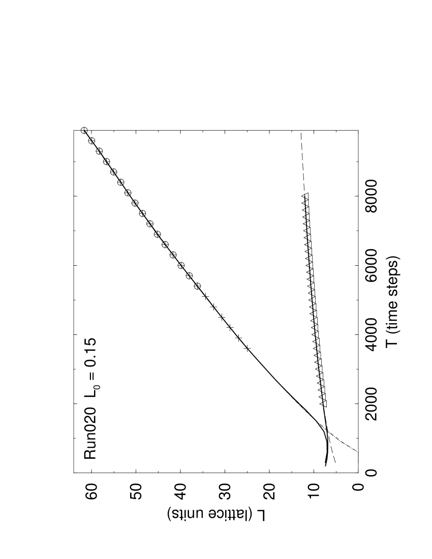
The characteristic length scale , defined via (19), has been calculated for the eight runs in table 2. The order parameter data was coarse-grained to before analysis, but comparison with smaller runs confirmed that there was no effect of this on within the ‘good data’ range. The latter is defined as , with fixed by our criterion on residual diffusion (§ 8.3) and as required to exclude finite size effects (§ 8.5). Figure 6 illustrates how the fitting was done.
To parameterize the time dependence of , the ‘good data’ was fitted, for each run separately, to the following form
| (61) |
(equivalent to (27)) where , and are fitting parameters.

A nonlinear curve-fitting utility was used to create the fits, which all fell within a specified tolerance of 1%. However, some trade-off is possible between the three fit parameters and a realistic uncertainty estimate for the exponent, , is around 10% for the first three runs in table 2, and 5% for the rest. The fits are shown in figures 7 and 8, which also shows the diffusion-only data used to determine as described in § 8.3. The fitted results are summarised in table 5.


| fits at 2% diffusion | fit | at diffusion | fit 1% | ||||||||||||
| Run | 2% | 1% | |||||||||||||
| Run028 | 36 | 0 | .88 | 0 | .0096 | 1948 | 0 | .41 | 20 | .0 | 28 | .5 | 0 | .81 | |
| linear fit | 1 | .0 | 0 | .00028 | 516 | ||||||||||
| Run022 | 5 | .9 | 0 | .86 | 0 | .023 | 304 | 0 | .64 | 26 | .0 | 38 | .0 | 0 | .88 |
| linear fit | 1 | .0 | 0 | .00605 | |||||||||||
| Run033 | 5 | .9 | 1 | .16 | 0 | .0012 | 442 | 0 | .48 | 17 | .5 | 24 | .9 | 1 | .12 |
| linear fit | 1 | .0 | 0 | .0060 | 1445 | ||||||||||
| Run029 | 0 | .95 | 0 | .95 | 0 | .0175 | 1020 | 0 | .54 | 15 | .3 | 21 | .7 | 0 | .92 |
| Run020 | 0 | .15 | 0 | .80 | 0 | .0418 | 603 | 0 | .60 | 23 | .4 | 34 | .9 | 0 | .80 |
| Run030 | 0 | .01 | 0 | .75 | 0 | .0747 | 1362 | 0 | .51 | 14 | .8 | 22 | .4 | 0 | .76 |
| Run019 | 0 | .00095 | 0 | .67 | 0 | .134 | 1008 | 0 | .60 | 21 | .5 | 33 | .8 | 0 | .66 |
| Run032 | 0 | .0003 | 0 | .69 | 0 | .0833 | 1855 | 0 | .48 | 19 | .0 | 29 | .8 | 0 | .69 |
The data show values ranging from 1.12 to 0.66 with a decreasing trend as is decreased. Certainly, an increasingly negative curvature of the plots with decreasing is apparent from figures 7, 8. However, the resulting fit parameters were relatively erratic for the three runs of largest (expected to lie in the viscous regime). Indeed, we found and for two runs with the same nominal . This was partly due to a relatively ill-conditioned fit as can be appreciated from figure 7. (A second possible cause of the erratic fits is the presence of long-range velocity fluctuations; see § 8.5.)
Therefore it was decided to refit the data for the three most viscous runs, imposing , the anticipated value. This yielded much better consistency among the fitted values of , which with viscous scaling should obey , where is universal; with the forced linear fits this was indeed the case with extracted as for the three runs under discussion. Subject to this, we obtain a range of values of from 1.0 (Run028, Run022 and Run033) to 0.67 (Run019), with intermediate exponents 0.95 (Run029), 0.80 (Run020) and 0.75 (Run030) at intermediate . This suggests that the simulations have indeed covered the viscous, crossover and inertial regions. However, the ultimate test of this is to convert to reduced physical units and construct the curve explicitly.
9.3 Universal scaling plot for
Our method for combining the data from different simulation runs to give the curve follows Jury et al. (1999b). As apparent from definitions (1), the only fit parameter that is actually needed when converting data to reduced physical units () is the intercept, . Then one uses the known density and viscosity, and the measured interfacial tension, to complete the conversion.
Figure 9 shows the data from all the runs in table 2 combined on a single log-log plot. Note that for the two runs of the resulting data collapse is much improved by the forced linear fit (giving two very different values of the nonuniversal offset instead of two disparate values of ). With the former, the two datasets overlie on the plot but with the latter they do not; this helps to vindicate our choice of fit. Apart from a similar reservation about force fitting for the most viscous run (), the curve is free of adjustable parameters. Although we did not have resources to cover the entire curve with data, there is no evidence for any breakdown of universality: the various runs do appear to lie on a smooth underlying curve. (In particular, the two most inertial runs virtually join up.)

The apparently universal curve shows scaling that is first linear (, with ), then passes through a broad crossover region before reaching (with ) at large , . The positions of the crossover and inertial runs on the graph are in keeping with the trend for the scaling exponent, , fitted directly from each run. This confirms that the exponents determined from our fitting procedure do accurately reflect what is going on in these simulations. The extreme breadth of the crossover regime, , justifies the use of a single exponent to fit each run (27), (61) even in the crossover: no single run is long enough to see a change in exponent from beginning to end beyond the estimated errors. There is no hint that the exponent is reducing still further to , as predicted by Grant & Elder (1999), although a further crossover beyond the range of reached in these simulations cannot be ruled out.
Recall that intersection of asymptotes on the plot defines , the characteristic crossover time from viscous to inertial behaviour. As mentioned previously (§ 4), scaling theory says only that is ‘of order unity’. The measured value is close to , a value that should raise no eyebrows in the turbulence community but may do so among workers in phase separation kinetics. Since is very close to , the largeness of can be traced to the smallness of and to the relatively minor change in exponent on crossing from viscous to inertial scaling: for by its definition, where subscripts signify viscous and inertial values.
Note too, the huge range of scales covered by the combination of eight simulation runs: five decades of length and seven decades of time. This achievement is only possible by fully exploiting the expected scaling. This means that, although our work is capable of falsifying the scaling hypothesis (our plot might not have joined up, and might yet not do so when more data is added), its non-falsification in our work may not represent persuasive proof that the scaling is true.
For, as mentioned previously (§ 7), to navigate the curve we are forced to correlate the simulation parameters in a systematic way. Hence if the coarsening rate was in fact dependent on , say (for example by being pinchoff-limited, Jury et al. (1999b)), this would not necessarily show up as bad data collapse in figure 9, since is strongly correlated with and/or . In principle, however, our parameter steering has no effect on data within a run, so that any ‘steering-induced’ data collapse could in principle be detected because curves would not quite line up with their neighbours on the plot, although their midpoints would lie on a smooth curve (Jury et al., 1999b). Although we believe this is not happening for our data, we do not have enough results to entirely rule it out, especially as something similar does occur in our own velocity derivative data (§ 11).
Our results for the evolution of the interfacial structure are compared with those of previous authors in Appendix B.
10 Results for the fluid velocity
Due to data storage limitations for the largest () runs, our velocity analysis also made extensive use the runs listed in table 3. The velocity field was analysed as a single, continuous field, filling the whole simulation; there is no explicit information about the location of the interface between the two fluid phases. However, visualisation of the velocity field was done using the AVS package and examples (one viscous, one inertial) are shown in figure 10, where the flow patterns can be compared with the domain structure defined by the interface.
viscous interface viscous velocity
inertial interface inertial velocity
vorticity + interface turbulence velocity
There are almost no prior data on fluid mixtures with which to compare these results. A simulation using a pseudospectral method written by Young (1999) was therefore used to generate a velocity field for single fluid, freely decaying turbulence with a similar Reynolds number to those of the spinodal system in the inertial regime. A velocity map for this single fluid turbulence is also pictured in figure 10.
A trend from locally laminar flow to more chaotic motion is apparent in passing from the viscous to the inertial regime. The vorticity map in the latter case is comparable to the one for the turbulent single fluid (not shown). However, the comparison is hindered by the fact that the interfacial motion at length scale introduces a ‘whorly’ velocity pattern even in the purely viscous flow regime. A better discriminator between the two regimes, pursued elsewhere, comes from watching the time evolution of the interfacial structure itself, which is clearly underdamped in the inertial case, Desplat et al. (2000b).
10.1 Velocity structure factor
The velocity structure factor was introduced in § 8.4. For numerical purposes we define it (following (59)) as
| (62) |
The results were shown already in figure 4, where is depicted for three of the runs in table 3, alongside two calculations (LB and spectral) for single fluid turbulence. These structure factors are in unscaled units but in each case correspond to a point during the run where the domain size is around 30 lattice units.
The bumps on the curves at high were discussed in § 8.4. But even apart from these, the velocity structure factors have very different shapes in the viscous (Run027), crossover (Run018), and inertial (Run031) regimes; these differences are much larger than for the order parameter structure factor (figure 5). In other words, the geometry of the fluid flow is changing much more significantly, as one moves along the curve, than the geometry of the interface.
We return to this in § 10.2, but first address an issue raised in § 8.5, which is the apparent divergence in at low in the viscous regime. This can be qualitatively explained as follows. In a purely viscous approximation (Stokes flow) the NSE (17) becomes in Fourier space
| (63) |
Here contains the chemical term which is mainly localised on the interface between the two fluids. We now argue that this term is strongly correlated at length scales up to the domain size but not larger ones: this means that, for the purposes of low wavenumbers () it is a random variable with short range correlation. Ignoring for simplicity all tensor indices, one thus has , a constant, as . From (63) we find immediately
| (64) |
Thus the long range, Stokesian hydrodynamic propagation converts short range fluctuations in into long range fluctuations in the fluid velocity. As mentioned in § 8.5, the resulting divergence could lead to erratic coarsening rates and/or problems with finite size effects, throughout the viscous regime. This appears not to have been noticed by previous authors.
There is a somewhat related anomaly that arises in colloidal suspensions under gravity, although in that case the short range fluctuations are in the density, which is effectively a random body force, rather than in a random stress: Segrè, Herbolzheimer & Chaikin (1997).
10.2 Length scales from the velocity field
The velocity structure factor, , can be used to calculate a velocity length scale, analagous to (compare (19)):
| (65) |
This length measure was found to be insensitive to coarse-graining in nearly all cases. Data collected for from the runs was converted to reduced physical units, using the values of already obtained from the fits and given in table 5. (Hence no further fitting was involved.) The resulting scaling plot is shown, alongside the data presented earlier, in figure 11 (left).

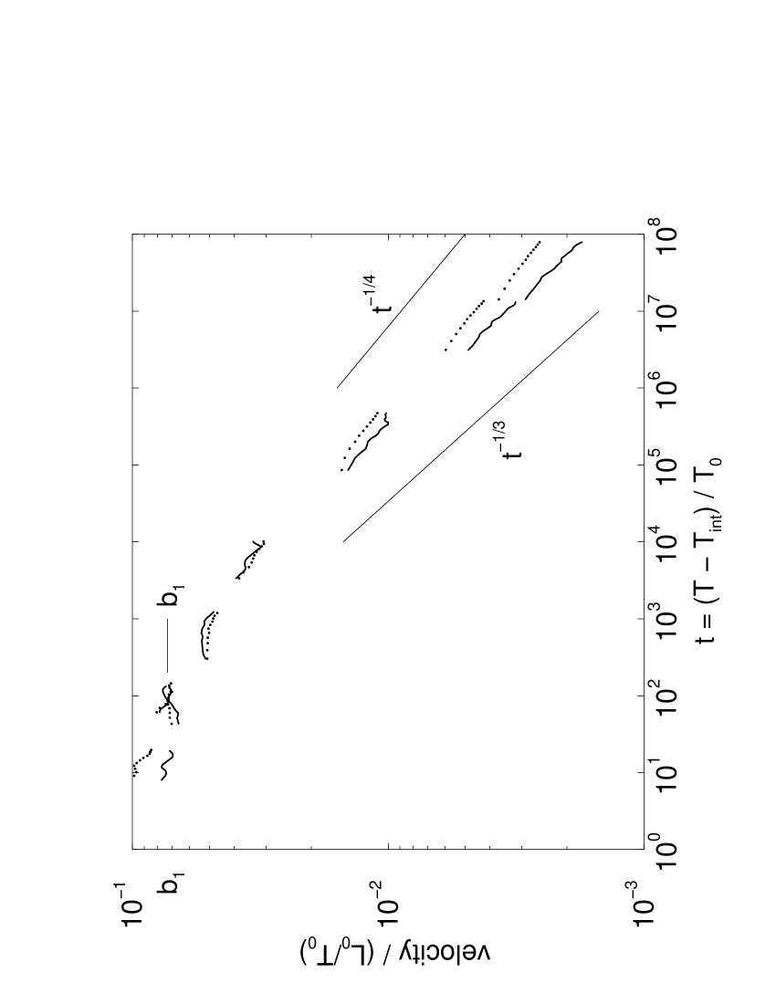
The results in the inertial regime show a strong convergence between and : the velocity length shows the same scaling as , with a similar prefactor. This is not obvious a priori, since, as mentioned above, the shapes of and are very different.
More surprisingly, we find that to a fairly good numerical approximation, shows a growth throughout the crossover region, and that this even extends far into the viscous regime, within which exceeds the domain scale by a significant factor. However, as the viscosity is increased to access the bottom left corner of the plot, the data are increasingly affected by finite size effects, since then is comparable to the system size . These are especially pronounced for the most viscous run (with almost constant during that run). Allowing for these effects, the data is consistent with at all times; however we have no reason to expect this result in the viscous regime, where both the simple and the extended scaling analyses (§ 4, 5) predict instead . Note, though, that the velocity length measure chosen (65) is sensitive to the low divergence found above in , which would give a contribution of order from the lower limits of integration. It is possible that for the parameters and system sizes used here, this size-limited contribution combines with those from higher wavevector to give an apparent power in the viscous regime.
Alternative length measures may be had by taking the ratio of two other successive moments of , to replace (65). Adding one extra power of to the top and bottom integrand gives a length measure that lies between and throughout the viscous regime, reducing the exponent discrepancy there, but without attaining the linear scaling of itself. For more than two extra powers of the scaling gets worse, not better, as the integral in the denominator becomes dominated by high contributions.
10.3 Average velocities
The rms fluid velocities (spatially averaged) were calculated for all the runs in table 2 and are plotted in reduced physical units in figure 11 (right), alongside the reduced interface velocity derived from the order parameter.
In the most viscous run, Run028, the rms fluid velocity is larger than the interface velocity. Both velocities are fluctuating quite far from the expected constant behaviour in the linear region, and the fluctuations are more or less in step. This may in part be a facet of the erratic, finite-size limited behaviour seen in the far viscous regime (§ 8.5).
Otherwise we observe that the rms fluid velocity matches the interface velocity in the viscous and early crossover region, but grows larger than it in the inertial region, by about 40% at the largest . The two most inertial runs (Run019 and Run032) appear to have the rms velocity scaling with a slightly different exponent than the interface velocity (approximately as rather than ), though this may not be significant. Such a deviation is foreseen by neither the simple nor the extended scaling theory, both of which have velocities scaling as at all times. It would imply a buildup of kinetic energy in the fluid beyond that predicted by either scaling analysis. The excess may be caused by our approaching the limits of numerical accuracy in resolving velocity gradients with a consequent breakdown in energy conservation (see § 11.5, 11.8 below). A similar breakdown, caused instead by having too high a viscosity in lattice units (as indicated in § 7), may likewise contribute to the excess rms velocity seen in the most viscous run.
10.4 Velocity distributions
The pdf of the velocity components in a homogeneous, isotropic turbulent fluid is known to be almost Gaussian, and uncorrelated over large distances in both space and time. Non-Gaussian behaviour is found only in velocity increments and derivatives, (e.g. Monin & Yaglom, 1975).
The spinodal system is crucially different: it has a structural length scale , and correlations and inhomogeneity can be expected at this scale. Hence the velocity components themselves can show non-Gaussian pdfs. The departures are expected to show up through the fourth moment, since there is no preferred direction in space that would allow one to create a scalar from a third moment of velocity. (The third moment was checked and found to be close to zero.) The fourth moment is characterised by the flatness, , with a Cartesian index; this vanishes for a Gaussian distribution.


Figure 12 (left) shows the flatness for runs in table 3 as a function of time; a distinction is drawn between viscous runs (those with ) and crossover/inertial runs (with ). It can be seen that the flatness is quite variable, but as a general trend it grows slightly with time through each run, and also grows with decreasing (increasing inertia). The velocity pdfs show correspondingly wider tails and narrower peaks than for a Gaussian; an example for Run032 is shown in figure 12 (right). The shape is close to that found in the transverse velocity derivatives in the same system (shown dashed for comparison). These non-Gaussian effects are much more pronounced in the inertial than in the viscous regime.
11 Velocity derivatives
We now turn to the analysis of spatial derivatives of the velocity field. Velocity derivatives come in two types, longitudinal, e.g., , and transverse, e.g., or . Representative velocity derivatives (in fact, , , and ) were calculated. The differentiation was done by calculating etc., and Fourier transforming back to real space. The derivatives are unambigous so long as the gradients of velocity are small on the scale of the lattice spacing, but otherwise the resulting gradient is not the same as taking a lattice derivative (which we define via (55) with replacing ). In practice we have found signigicant () discrepancies the two methods; these were investigated in the context of energy conservation and are discussed further in § 11.5. For many purposes there is no particular reason to prefer the lattice to the Fourier definition and we retain the latter for simplicity.
11.1 Skewness of velocity distribution
In fully-developed turbulence the skewness of the longitudinal velocity derivatives approaches , (e.g., Monin & Yaglom, 1975). (The skewness of a variable is .) The transverse derivatives have zero skewness, by symmetry, but positive flatness.
Figure 13 (left) shows the skewness of the longitudinal velocity derivatives against time for the three most inertial runs in table 3. Also shown for comparison is the skewness from the freely decaying turbulence simulation.


In the two most inertial LB simulation runs, the skewness of the longitudinal velocity derivative reaches around . A plausible interpretation of this result is that patches of turbulence arise, but do not fill the whole system; if the patches have skewness , the overall value is less. From visualizations (see figure 10) we know that the interface remains smooth so that any turbulent regions should be in the middle of the fluid domains.
To test this idea further, a run with the same parameters was done, and at timestep 5000 (when the domain size was about 21, after residual diffusion had decayed to an acceptable level) the interface was suddenly removed by setting the order parameter to 1 throughout the system. This converted it into a single fluid with the same velocity field, which was then allowed to evolve. The longitudinal velocity derivative skewness for this run is shown in figure 13 (right), with Run031 and the single fluid turbulence data repeated for comparison. Once the interface was removed, the skewness quickly jumped to around from , providing strong support for the ‘turbulence in patches’ hypothesis; it appears that on removal of the interface, the turbulence rapidly infects the whole system. (Fairly soon after this, the system became numerically unstable causing the skewness to rise rapidly back toward zero as spuriously large velocities were generated; this is visible in figure 13, but was not investigated further.)
11.2 Reynolds numbers
In this work we choose to regard all Reynolds numbers as estimates of the rms ratio, , of the nonlinear term to the viscous term in the NSE (17), as defined in (29).
In practice, Reynolds numbers are usually constructed (via ) from a characteristic length () and a characteristic velocity (). In a homogeneously turbulent single fluid, the usual choice of velocity scale is . Also, the length measure must itself be constructed from the velocity field; various choices then arise. One is the integral scale, defined (to within prefactor conventions) as where is the total kinetic energy. (This a close relative of our , (65.)) A second is the Taylor microscale, , defined in Eq. (34). A third length is the Kolmogorov microscale, , (35), but this is not normally used to form a Reynolds number. In practice, most isotropic homogeneous turbulence simulation studies use as Reynolds number . This should give a reasonable estimate of the ratio , because as noted in § 5, is the length scale associated with the operator in . But note that, according to the extended scaling analysis (table 1), it is still not an accurate estimate asymptotically at late times: there one has the prediction that while .
In the spinodal system an obvious alternative to arises from choosing , the domain size, as the length scale; either or the interface velocity can then be used for the velocity scale. However, the resultings Reynolds numbers, , and (see (31)) are not directly comparable with , which is always much smaller.
All three quantities are shown as functions of the reduced time in figure 14 (left).


There is little difference between and ; both show reasonable scaling, with the deviations in the most extreme runs stemming from those discussed already in § 10.3. The large asymptote for in the inertial region is approximately as predicted by both the simple and the extended scaling analysis (but questioned by Grant & Elder, 1999). Our simulations extend from , and the crossover region occupies the range . Thus in terms of (rather than ) the crossover is not, after all, quite so broad.
In contrast to and , the data for does not show good scaling behaviour. The overall trend is of linear scaling in the viscous region and slower growth at around in the inertial region; both are broadly consistent with the extended scaling theory (see table 1). However, the individual runs do not line up onto a single curve. This non-scaling behaviour of can be traced to that of itself, which is examined in more detail in § 11.8.
11.3 Ratios of terms in the NSE
Shown in figure 14 (right) are the actual rms ratios and defined in (28) and (29) respectively. (Recall that the latter is the ratio of nonlinear to viscous terms in the NSE, which is what we believe a Reynolds number should estimate.) In order to form these ratios, one must first evaluate (rms values of) the three relevant NSE terms, , and , which are vector quantities at each point in space. An rms value is calculated as, , where , , and are the Cartesian components of the vector (for example), and the average is taken over the whole system. The first and second order spatial derivates of the velocity were found from -space data (as in § 11.1) on and runs; a further complication is that to evaluate , velocity data from consecutive time steps is required. Due to data storage constraints, this was only collected for a set of runs. This is large enough to obtain values for a domain size just larger than , but not to determine its time dependence accurately within any particular run; checks were made for consistency by comparing other quantities with data.
The values of and shown in figure 14 (right) lie between and but are closer to the latter. The two ratios remain the same order of magnitude as each other throughout, but vary by three orders of magnitude, from at the viscous end (indicating the viscous term is dominant by two orders of magnitude) to at the inertial end (indicating that the inertial terms are dominant by one order of magnitude). Though we cannot calculate it directly, is presumably somewhat higher (about 20) towards the end of our most inertial run. This confirms the claim made in § 9 that our simulations have reached a regime where the inertial terms are dominant in the dynamics.
Looking more closely at the behaviour of relative to , there is a significant difference in the crossover region, by around a factor of two (). Then, in the inertial regime, becomes less than by about 50% and appears to be heading for a lower growth rate. This deviation suggests that the asymptotic behaviour of these two ratios is perhaps going to be different. That would be consistent with the extended scaling predictions which are (table 1) that while constant; but if so neither curve is close to its final asymptote yet.
That the LB simulations are still far from the final asymptotic behaviour in our most inertial runs, even though inertial terms are clearly dominant there, is not unreasonable. The largest ratio actually achieved in our simulations is, by turbulence standards, still a fairly low Reynolds number. If the extended scaling theory of Kendon (2000) is correct, the final asymptotes for quantities relating to fluid velocity cannot be attained until an appreciable ‘inertial range’ has developed between the interfacial driving scale , and the smaller scales (, ) where energy dissipation is taking place. However, to observe scaling of for the structural (as opposed to velocity) data, it may not be necessary that the inertial cascade is fully established; one might only require that a reasonable degree of decoupling between interfacial motion and viscous dissipation has taken place. Our results for suggest that this has already happened by the time .
11.4 Structure factors of the NSE terms
Further information on the behaviour of the NSE terms can be obtained by calculating the structure factor for each term. (These are where or .) Results for one viscous and one inertial run are shown in figure 15.


Looking first at the viscous run, the structure factor of the viscous term takes the form of a broad peak stretching from a small bump at wavelengths around 12 lattice units (which is around half the domain size, ), down to the interface width, . Thus the dissipation is taking place over the smaller length scales in the system. (The small bump is a manifestation of the domain size in the dynamics; it is present at around throughout the run.)
In the inertial regime, the viscous term is, as expected, smaller than the inertial terms. The viscous term is similar in shape to that in the viscous regime, with the addition of two large peaks at high that presumably arise from the presence of the interface (compare § 8.4) and/or lattice effects. This suggests perhaps that the largest dissipative forces, and therefore most dissipation, are happening close to the interface (or at least on that length scale). The acceleration term has a broad peak in the structure factor at wavelengths around , and tails off quite sharply below 10 lattice units. The nonlinear term has a structure factor with a broad peak centred around 15 lattice units, intermediate between the length scale of the interface, , and the dissipation length scales.
The overall picture, though not quantitative (in view of the numerous sources of uncertainty, especially in the velocity derivatives) is qualitatively consistent with the extended scaling picture, in which the nonlinear term transports energy from large to small scales, where it is then dissipated. But in these runs there is still considerable overlap between the length scales for each term, as expected at relatively low Reynolds number.
11.5 Energy conservation, dissipation rate
The dissipation rate is crucial to the energy balance in the simulation. The LB algorithm is isothermal, and therefore does not strictly conserve energy, in that the energy dissipated as heat by the viscous stresses is taken out of the system locally rather than having to diffuse thermally to the boundaries. Nonetheless, the simulation should faithfully recreate the energetics of the isothermal Navier–Stokes equation, driven by interfacial motion (as in (17)), which makes precisely the same assumption. In the inertial regime, the interfacial energy should first be transformed into kinetic energy of the fluid; the observation of (see § 9.3) shows that this is happening at roughly the expected rate. To complete the energy balance, energy must also be removed from the simulation at the correct rate through viscous dissipation. This requires accurate modelling of the smaller length scales () at which such dissipation is taking place.
The dissipation rate can be calculated directly from the velocity data as
| (66) |
where the angle brackets are spatial averages and both the incompressibility () and homogeneity () of the binary fluid system have been exploited. The second expression is tantamount to using the Fourier definition of spatial derivatives, and as mentioned previously, this need not coincide with lattice derivatives when gradients are not small. Therefore the dissipation rates were calculated first using the Fourier space expression in (66) and then, for some but not all runs, using the real space expression with the lattice gradient operator as defined in Eq. (55).
The two estimates (Fourier and lattice) of the dissipation rate were compared with the rate of decrease of the sum of the interfacial energy and the fluid kinetic energy in the system: these should balance, once the interfaces are well formed and residual diffusion has become negligible. (Note that diffusion introduces its own contribution to the dissipation, not accounted for in the NSE, which may dominate early in each run.) We found that the lattice derivatives gave better agreement than Fourier ones in this comparison. However, even with these, the results were never more than satisfactory; best in the crossover region (within 25% of the expected value) but giving dissipation rates well above those required by energy conservation in the viscous regime, somewhat below in the inertial. At the viscous extreme the discrepancies were a factor three or more. Even in the crossover region, there was a tendency for the computed dissipation rate to drift below that required for energy conservation. Examples are shown in figure 16.
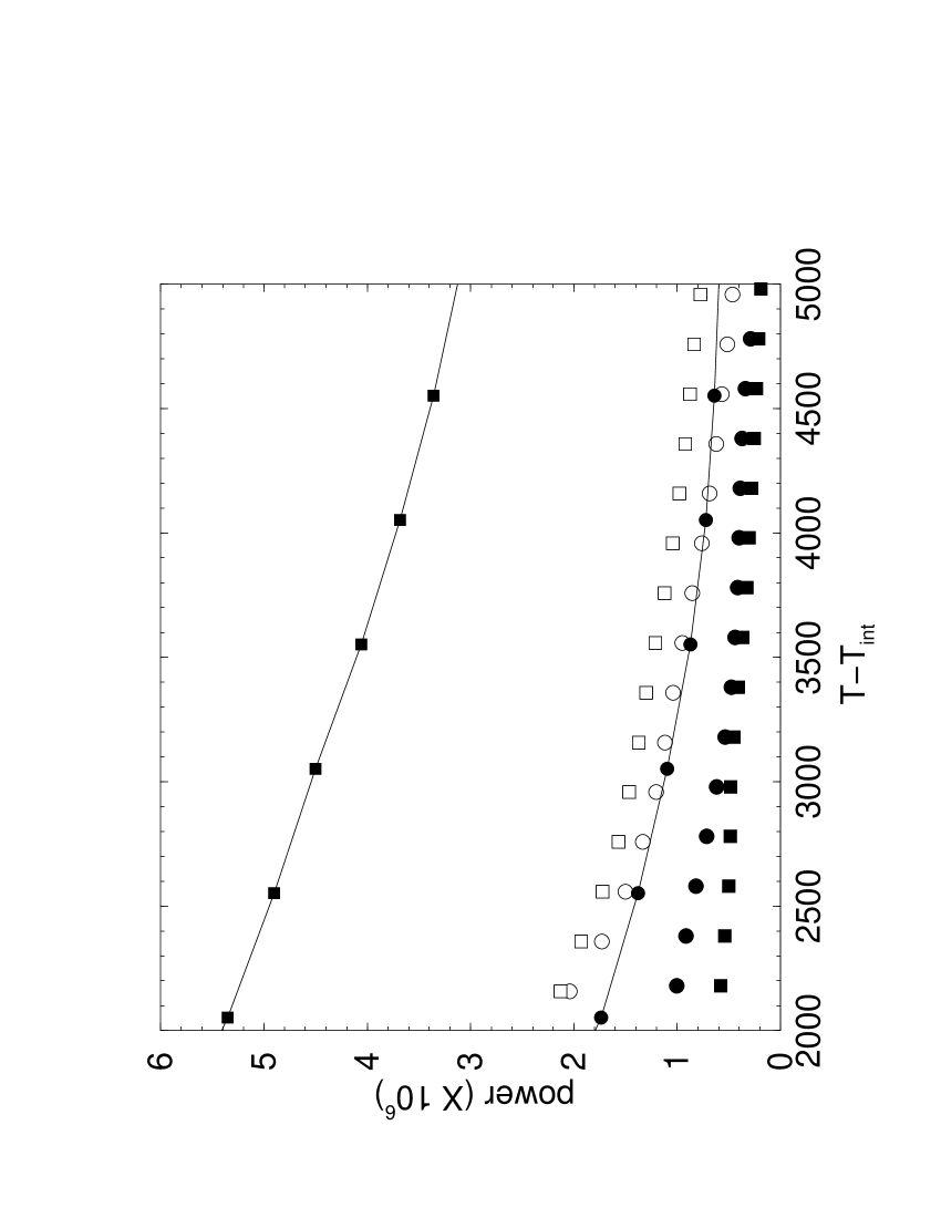
Use of Fourier derivatives to estimate the dissipation rate instead gave values that were consistently too high, through all regimes, by a factor 2 or so for runs in the crossover and inertial regimes and much more than this in the viscous regime.
A check was made to ensure that these discrepancies in the dissipation rate did not arise from compressibility effects, by computing the full expression for , without assuming fluid incompressibility as was done in (66). (See Landau & Lifshitz (1959) for the relevant expression.) This check was done with lattice derivatives; the results did not differ appreciably from the lattice version of Eq. (66), so that compressibility is not responsible here.
The fact that the two methods of finding derivatives differ, shows that dissipation is primarily taking place at short scales (of order a few lattice spacings). The results do not imply that LB is failing to conserve energy, but do show that the viscous dissipation actually generated by the algorithm is not accurately estimated from the Fourier derivatives; the lattice difference estimates for are better, but still not accurate. In principle even these need not give the true dissipation since the LB algorithm actually dissipates energy by relaxing the velocity distribution functions (41), and not by calculating lattice gradients. Note, in any case, that for qualitiative comparisons between runs (requiring log-log plots covering many decades) the factor two difference between Fourier and lattice derivatives is barely detectable, and we ignore it, for those purposes, below.
For the dissipation rate itself, simple scaling theory predicts that will always scale as . Kendon (2000) predicts the scaling to be in the viscous region, but in the inertial region (table 1). A scaling plot of the (Fourier) dissipation rate (in reduced physical units, as usual) is shown in figure 17 (left).


To the accuracy we are working, these data barely discriminate between the two scaling predictions though the upward curvature may slightly favour that of Kendon (2000). There is some sign in the viscous regime that the rate increases too fast; this might be connected with the velocity anomalies discused previously (§ 10.1).
11.6 Taylor and Kolmogorov microscales
The Taylor and Kolmogorov scales were defined in (34) and (35) respectively. Figure 17 (right) shows in simulation units for each run in table 2 and table 3. Values are evaluated mid-run at time such that the domain size , but plotted against the reduced physical time. The curves thus have the same shape as a scaling plot of and (since is here fixed in simulation units) but also allows the values to be compared with the lattice spacing (unity) and the linear system size (128 or 256). Given the expected effects of coarse-graining on the data at short length scales, the agreement between the two lattice sizes is satisfactory but only the data is discussed in what follows.
As can be seen in figure 17 (right), does not vary by much between runs, although it is roughly a factor of two larger in the crossover region than in the viscous and inertial extremes. The extended scaling analysis (table 1) predicts that in the inertial region, and the data is broadly consistent with this; an asymptotically constant ratio, predicted by simple scaling, is marginally less plausible though not ruled out. Likewise, is not far from the prediction of the new scaling theory (), and perhaps somewhat further from that of simple scaling (). For the viscous regime, however, does not appear to scale as , nor does approach a constant, as predicted by both scaling theories. Once again the low velocity anomaly (§ 10.1) in the viscous regime could be to blame for this, but so could inaccuracies in the estimated dissipation rate (§ 11.5).
11.7 Resolution of the energy cascade
The Kolmogorov microscale has a further significance for any attempt at numerical simulation in inertial fluids. In a fully turbulent fluid, is expected to be smaller than , and to mark the smallest length scale relevant for dissipation. This should, if the results are to be relied upon, be ‘resolved’, that is, should lie above the discretization scale set by the lattice. There is some debate over exactly how small can be in relation to the lattice spacing, but a factor of 1.0 to 1.6 has been put forward; see for example, Eswaran & Pope (1988); Yeung & Brasseur (1991). Our best estimate for in the most inertial () run is around lattice units; values are higher in all other runs. However, in view of the quantitative uncertainty in our velocity derivative estimates (see § 11.5), this estimate is good to only a factor of 2 or so. Therefore, the most inertial of our runs is certainly close to the resolution limit, and we would not wish to proceed to higher without a larger system size. Note that only in that run is appreciably smaller than as expected asymptotically in a turbulent flow; but the Taylor scale is well-resolved, by the same criterion, in all runs.
However, estimates of how well the cascade is resolved using these two lengths could be misleading, in that they assume local as well as global homogeneity. So if, for example, most of the dissipation were to occur in a thin layer around the interfaces in the system, the globally averaged might suggest that the dissipation was fully resolved whereas in fact it was not. This would be consistent with our findings (§ 11.5) that the actual dissipation rate in LB is poorly estimated from the Fourier velocity derivatives, and imperfectly even from lattice ones.
On balance, we believe that the energy cascade is adequately resolved in most of our LB simulations, at least for the purposes of getting the correct evolution of the structural length scale . (As noted in § 11.3, a fully resolved cascade might not be needed for this, so long as there is sufficient decoupling of interfacial motion and viscous dissipation.) However, the most inertial runs may well be marginal in terms of resolution; in common with several other aspects of the simulations (such as the residial diffusion, and anisotropy), these runs are at the limit of what is possible using this simulation method with current computational resources.
11.8 Apparent scaling violations
In our various analyses of the velocity derivatives, we focused mainly on scaling plots made by taking a representative ‘mid-run’ data point from each LB simulation run (e.g. figure 17, left). These plausibly connect to form a smooth curve. However, one test of scaling is whether the full datasets (rather than a representative point) from different runs appear to join up smoothly when plotted in reduced physical units; this was satisfactorily the case for the structural data (figure 9) and reasonable also (though not by any means perfect) for the velocity data (figure 11, left), and (figure 14, left).
However, the expected scaling within runs failed completely for (also in figure 14, left). This quantity differs from the others just mentioned in that its definition involves , which in turn involves the dissipation rate (see (34)) and therefore depends on velocity derivatives. More generally, we find similar ‘scaling violations’ in all the quantities we have looked at that involve calculating velocity derivatives. Figure 18 shows this for (left) the various rms terms in the NSE and (right) the Taylor and Kolmogorov scales. The dissipation rate (not shown) shows similar features.


Apart from the failure of the runs to join up, the data for the NSE terms is in reasonable accord with the scaling predictions (table 1) for the viscous term of in the linear region and or in the inertial region, and for the inertial terms of or in the inertial region. Even the scaling of for the nonlinear term in the viscous region is as predicted by the new scaling theory (Kendon, 2000). However, within each run the quantities are falling more slowly than all these predictions. Similarly and do not scale within single runs in the same way as they scale between runs, except perhaps in the middle of the crossover region. (The same is true of , the dissipation rate, from which is derived.)
At present, we have no simple explanation of these apparent scaling violations. They could perhaps be a sign of subtle nonuniversalities of the type suggested by Jury et al. (1999b), though it would certainly be premature to conclude this without similar (though perhaps less severe) effects being detected in . Another possibility, noted previously (§ 11.5, 11.7) is that the we are not able, using LB with these system sizes, to fully resolve the velocity gradients that arise.
On the other hand, our velocity derivatives do not appear to be completely lattice controlled, since for example, in (66) one could then set . This would give , giving in the inertial regime within each run (which is about right) but in the viscous regime , and also throughout both regimes, neither of which is plausible for our data (see figure 18, right). We have made various further attempts to explain the data by assuming ‘composite’ scalings, based for example on the idea that dissipation occurs mainly near the interface where velocity gradients might be anomalously large ()555We note that in a very recent analysis, Solis & de la Cruz (2000) developed an heuristic alternative to that of Kendon (2000) in which dissipation takes place in an (asymptotically) thin layer around the interface rather than in the bulk. They argue that coarsening is limited by the damping rate of capillary waves of wavelength , and that this damping rate is unaffected by nonlinearity; this gives . We find no evidence for this in our data. Using the oscillation frequency instead of the linear damping rate recovers .. In that case, one would have , where the factor is the volume fraction of interface. Although none of these attempts was successful, an explanation along these lines is not completely ruled out.
One further complicating factor is that, within LB, the fluid viscosity is frequency dependent: the Navier Stokes limit requires that velocities are not only small (in lattice units) but also evolving sufficiently slowly. For very low viscosities, approaches which means that the distribution function is over-relaxed (nearly reversing sign at each time step), see Equation 42. (In effect, the ‘natural’ viscosity scale in LB is of order unity and the over-relaxation is used to create an unnaturally small value.) This works successfully if accelerations are small but could result in a higher dissipation rate than would be the case for a purely newtonian fluid, especially in the most inertial runs.
12 Conclusions
Our LB results for symmetric binary fluids, undergoing spinodal decomposition after a deep quench, appear to confirm the dynamical scaling hypothesis, which requires a universal time dependence of the structural length scale when expressed in reduced physical units as a function of time, (figure 9). We found no signs of nonuniversality here, although some weak breakdown of it, as suggested by Jury et al. (1999b), cannot be entirely ruled out. By exploitation of the expected scaling, and careful parameter steering and validation tests to eliminate residual diffusion and other unwanted effects, we achieved an curve spanning seven decades of reduced time and five of reduced length . The curve asymptotes to at (the viscous regime), with , and at (the inertial regime), with . On our reading of Guenoun et al. (1987), is within 10% of the most careful experimental measurements (albeit not for a deep quench) although others (Laradji et al., 1996) extract an estimate about twice as large from the same experimental results.
The crossover time, in reduced physical units, as defined by the interception of the viscous and inertial asymptotes, is surprisingly large (). So is the width of the crossover region (four decades). This may explain why the region has never yet been confirmed in laboratory experiments. The default assumption that is ‘of order unity’ would mean that for fluid pairs typically studied (short chain alcohols and water for example), the inertial regime could be accessed at length scales of a few microns, easily studied by light scattering. But in fact, to exit the crossover region (at ) one needs which for typical fluids gives of order centimetres (and larger still for the near-critical quenches often used, see Guenoun et al. (1987)). This requires direct visualisation experiments, not light scattering, and more importantly requires rigorous exclusion of thermal convection and gravitational effects. The latter is likely to be possible only with extremely careful density matching, or in microgravity, Cambon et al. (1997).
Our findings are less extreme when translated into Reynolds numbers. The conventional definition of the Reynolds numbers for the spinodal problem is ; the crossover regime then spans and the Reynolds number range we actually achieved was . (Note that we see no sign of a saturating as predicted by Grant & Elder (1999), but cannot rule this out, at some value well above 350. )
These figures are reduced further if the actual ratio of nonlinear to viscous terms is used as the Reynolds number; our results span . At the upper end of this range, we have described in detail the first unambiguous simulations of a regime in which the inertial terms in the Navier–Stokes equation are actually large compared to the viscous ones; here we observed . However these simulations may still be far from the asymptotic regime addressed by the scaling analysis of Kendon (2000), in which ultimately one expects for the Kolmogorov, Taylor and structural length scales. But in fact, although is only slightly smaller than even for our most inertial run, our data for the inertial regime is already somewhat more consistent with Kendon’s analysis than with the simpler (single length scale) scaling predictions of Furukawa (1985).
In the viscous regime, we recovered the expected () scaling though this is somewhat erratic and accompanied by an unexpected behaviour of the velocity correlation length (figure 11, left) and possibly also the dissipation rate (figure 17, left). The first of these, at least, may be related to the presence of anomalous long-range correlations of the velocity over length scales much larger than the domain size . These were detected numerically in our most viscous runs, and can be explained simply by assuming that the interfaces contribute a random stress with local correlations on scale (see § 10.1). It is quite possible that such effects have arisen undetected in previous simulations of the viscous regime; in principle they could lead to finite size problems arising long before the domain size approaches the size of the simulation cell. Fortunately, the same does not appear to happen in the inertial regime.
As well as through their differing domain growth laws ( or ) the viscous and inertial regimes can be distinguished by rather subtle changes in interface geometry (evident through the structure factor and by visualisation, with more thin necks in the inertial case) and by much larger changes in the velocity statistics. For example, the velocity pdf is significantly flatter for inertial than for viscous runs and also there is significant skewness for longitudinal velocity derivatives in the inertial regime. In that regime, we achieve results that show some of the characteristics of a turbulent fluid, although non-Gaussian features are seen directly in the velocity distribution as well in that of derivatives. This reflects the presence of microstructure (interfaces), as well as some turbulence, in the fluid mixture.
The scaling of quantities involving velocity derivatives was found to give reasonably continuous curves when mid-run values were plotted in reduced physical units (e.g. figure 17, left) but showed apparently systematic violations of the scaling behaviour which that would imply, when analysed in detail within each run. This could indicate some physical nonuniversality, or some shortcoming of the LB code; but equally it can be attributed to uncertainties over how to accurately estimate derivatives that are not small on a lattice scale. The LB code is implicitly aware of differences in the local velocity distributions but does not itself calculate velocity derivatives. Therefore, when these derivatives are not small, there can be discrepancies between their ‘effective’ values (as defined, e.g., through the actual dissipation rate generated by the algorithm) and any estimate based on Fourier, or lattice difference, data.
The fact that such ambiguities arise at all is an indication that our LB simulations are close to the limits of accuracy acceptable for the fluid motion, since ideally all gradients encountered in LB should be small, not large, on the lattice scale. It is interesting that they arise even when the Taylor and Kolmogorov microscales, and , are both significantly larger the lattice spacing; this perhaps suggests heterogeneity of the velocity field that is stronger than in single-fluid homogeneous turbulence. It may mean that, despite our best endeavours, we have not adequately resolved the fluid motion at short length scales. Fortunately, according to the analysis of Kendon (2000), the main requirement for observation of in the inertial regime is that the interface motion is decoupled (by fluid convection) from the dissipation scale, and not that the latter is modelled with complete accuracy. The reason is that, once the interface is decoupled, its motion is controlled by how fast it feeds kinetic energy into the fluid at large scales; the precise details of the dissipation further down the cascade has no further influence on the interfacial dynamics. If so, statistics based on the domain growth law may be much more robust than those for the fluid velocity and (especially) velocity derivatives, in the inertial regime.
Very similar accuracy limits were also reached in the thermodynamic sector, where we required narrow interfaces, with large composition gradients, to satisfy the conflicting requirements of rapid interfacial equilibration and low residual diffusion. (This gave interfacial tensions 10-15% different from nominal, with measurable lattice anisotropy.) We have taken unusual care to analyse (and maintain under reasonable control) the various sources of error. The reader has, we hope, enough information to decide for herself how much confidence to place in our various results.
It is interesting to ask how simulations might be taken further into the inertial regime. If the analysis of Kendon (2000) is any guide, the ultimate asymptotic state entails, computationally, resolution of the following scale hierarchy:
| (67) |
with the lattice spacing, or, more generally, the density of degrees of freedom in the simulation. A factor 3 between each of these length scales is roughly what we achieve at . But a worthwhile improvement to give, say, a factor 10 between each would require . For a three dimensional system, this lies beyond any foreseeable innovation in computational hardware if any current methodology is used. Possibly the way forward would be to couple a coarse-grained algorithm (such as large eddy simulation) for the turbulent fluid to a moving interface; we leave this to others to explore.
Acknowledgements.
We would like to thank Alan Bray, Anatoly Malevanets, Alexander Wagner, Patrick Warren, Julia Yeomans and Alistair Young for helpful discussions. Work funded in part under EPSRC GR/M56234.Appendix A Analysis of hydrodynamic modes
In this appendix we analyse the hydrodynamic modes for the LB hydrodynamic equations (57-58). We take as our reference state one in which the fluid is at rest with uniform concentration. In this case, to linear order in the perturbation of the hydrodynamic fields the Navier-Stokes equation is satisfied, and only the spurious terms in the balance equation for the order parameter remain. Specifically, the equations we are going to analyse are
| (68) |
where and are the kinematic shear and bulk viscosities, respectively. Using eq.(2.9), the last term in the third equation can be rewritten as
| (69) |
where is the speed of sound and the chemical potential. This expression shows that there is a spurious coupling between the order parameter and gradients of the density field. Such a coupling can only be relevant when the binary mixture exhibits compressibility. In terms of the deviations of the hydrodynamic fields with respect to their equilibrium values, , eqs.(68) become
| (70) |
where we have defined . In Fourier space, this set of equations can be expressed in matrix form, setting as
| (71) |
where . The hydrodynamic mode eigenvalues are correspondingly
| (72) | |||||
| (73) | |||||
| (74) |
The first mode corresponds to the propagation of shear waves, the subsequent two modes are related to the propagation and damping of compressible momentum waves, and the final mode is related to the diffusion of the order parameter. One can see that the presence of the spurious term in the convection-diffusion equation does not qualitatively modify the propagation of the order parameter: it remains diffusive. However, its eigenvalue depends on the compressibility of the the fluid, and for a compressible fluid there is then a reduction of diffusivity coming from the coupling to sound waves. Such a coupling also modifies the propagation and damping of longitudinal waves in the medium, so that these become a function of the order parameter.
To whatever extent the compressibility of the fluid can be neglected, the additional coupling between the order parameter and the density becomes irrelevant, and the expected diffusion coefficient for the convection-diffusion equation of the order parameter is recovered.
Appendix B Comparisons with other work
In order to compare our results with others’ published work, a similar scaling procedure must be applied to place their data onto the universal scaling plot in figure 9. This is only possible for work reported in sufficient detail to enable values for and to be calculated. Recent three-dimensional work where comparison is possible includes that of Bastea & Lebowitz (1997), Laradji et al. (1996), Appert et al. (1995), and Jury et al. (1999b). These four sets of results are shown along with the LB data in figure 19. Simulations of three-dimensional spinodal decomposition with hydrodynamics for which quantitative comparisons were not possible include, Koga & Kawasaki (1991), Puri & Dünweg (1992), and Alexander et al. (1993), all of whom claimed to have simulated the linear regime; Shinozaki & Oono (1991), Ma et al. (1992), Lookman et al. (1996). The last two claimed to have simulated the inertial regime but offered no evidence beyond their fitted exponent values for definitely having inertial rather than diffusive effects.

The four studies for which detailed numerical comparisons are possible will now be considered in turn.
B.1 Bastea & Lebowitz (1997)
Bastea & Lebowitz (1997) carried out a three-dimensional simulation containing about particles whose motion was described mesoscopically by Boltzmann-Vlasov equations. They combined direct simulation Monte Carlo methods for the short range interaction with particle-in-cell methods for long range interactions. The fluid system is relatively low-density; they describe it as a gas-gas phase separation. The necessary fitting and scaling for the results reported by Bastea & Lebowitz was done by Jury et al. (1999b).
On the universal scaling plot, figure 19, the supposedly viscous-regime portion of the data from Bastea & Lebowitz is shown as circles. It lies in the correct (lower left) region of the graph, but well to the left of any of the LB results. The scaled value of the fit parameter, , from the refitting by Jury et al. is . This compares with the considerably smaller values from the LB results in the linear region. The dynamical scaling hypothesis requires however that should be universal to all systems in the viscous regime. The high reported leads us to suspect residual diffusion. Bastea & Lebowitz do not report the diffusion rate in their system in a form that can be used to apply the analysis of § 8.3, but test LB runs have been done with high diffusion rates that produce LB data sets very similar to those of Bastea & Lebowitz. Two such test runs, Run024 and Run010, are shown in figure 20.


On the left, Run024 is compared with Run028, one of the runs in table 2. Run024 has the same parameters as Run028 except for the mobility, which is eight times higher. Run024 fits a free exponent of , which is similar to Run022 (also in the linear region). However, the lack of an initial flat diffusive region (also absent in Bastea & Lebowitz (1997)) strongly suggests the diffusion is too strong for uncontaminated linear growth to be observed within the attainable system size. A linear fit to the upper part of the data produces a scaled value of , compared with 0.073 for Run028.
On the right, Run010 has a value of , larger than for any of the runs finally used by us, see table 3. This should put it even further into the linear region than the rest of the runs. However, a fit with a free exponent produces . A linear fit to the upper part of the data produces a value for the scaled fit parameter of , i.e. about the same as the data from Bastea & Lebowitz, which this curve resembles. It seems likely, therefore, that the data from Bastea & Lebowitz (1997) has strong residual diffusion, and the results they present are a mixture of linear and diffusive growth.
B.2 Laradji, Toxvaerd & Mouritsen (1996)
Laradji et al. (1996) used a large-scale molecular dynamics simulation of a Lennard-Jones model with 343000 particles with a deep quench. The necessary fitting and scaling for the data of Laradji et al. was done by Jury et al. (1999b). The results are shown on figure 19 as triangles lying, like those of Bastea & Lebowitz (1997), to the left of the LB data towards the lower left corner, again in the viscous regime according to the LB analysis. Laradji et al. claimed their results confirmed the linear scaling, but their value of the scaled fit parameter, , is again higher than ours. However, it is in well within the range of values spanned by the the over-diffusive LB runs shown in figure 20 (). The shape of their curve matches that of Run024 in figure 20 (left), i.e. there is no initial diffusive plateau before domain growth begins. In LB data this was always a sign that the run had too high a mobility and significant contamination by residual diffusion.
B.3 Appert, Olson, Rothman & Zaleski (1995)
Appert et al. (1995) used a three-dimensional lattice gas simulation to simulate spinodal decomposition. Their largest system size was and they also used to test for finite size effects; they rejected data with , whereas we saw significant finite size effects by this stage (and applied the stricter condition, ). They claimed a fitted exponent of , which, if correct, would put their results in the inertial regime. Taking the relevant interval of their data, refitting it by our method (giving an exponent ) and converting into reduced physical units gives the dataset (squares) on figure 19. This shows that, if our LB data is correct, the data of Appert et al. is actually in the crossover region. It appears to be asymptoting onto the LB data from above, which again suggests significant residual diffusion, giving too low a value for the fitted exponent. As with the data of Bastea & Lebowitz (1997) and Laradji et al. (1996), the plot is lacking the initial diffusive plateau, an absence that we found was invariably associated with strong residual diffusion within LB.
B.4 Jury, Bladon, Krishna & Cates (1999b)
Jury et al. (1999b) carried out a series of simulations of a symmetric, binary fluid mixture using the DPD (dissipative particle dynamics) method with particles and a deep quench. (The DPD algorithm combines soft interparticle repulsions with pairwise damping of interparticle velocities and pairwise random forces.) In terms of the range of domain scales that can be probed, as a multiple of the interfacial width, these are roughly equivalent to our runs using LB. These authors found that each data set was well fitted by a linear scaling, , but with a systematic increase of upon moving from upper right to lower left in the universal scaling plot, see figure 19 (inset). These seven data sets have a range of values, , which places them all firmly in the crossover region found in the LB results, between Run029 () and Run030 ().
Jury et al. suggested two alternative interpretations of their own data and that of Laradji et al. (1996) and Bastea & Lebowitz (1997), to explain the observed linear scaling within each run, but lack of consistency in the prefactor, . The first was a possible nonuniversality arising from the physics of pinchoff. The second was that all data sets formed part of an extremely broad crossover region. This explains the observed trend , but not the linear scaling within each run. However, Jury et al. noted the possibility of ‘dangerous’ finite size effects within their data, which was truncated at . Our LB results support the latter explanation for the DPD data, with a separate or additional reason (residual diffusion) for rejecting the other datasets. Unlike these, all the data sets of Jury et al. do lie very close to the LB results, see figure 19 (inset). Moreover, the DPD show a diffusive plateau prior to the onset of the apparent linear regime, consistent with low residual diffusion levels.
Since the DPD simulation method is very different from LB, the correspondence of the two sets of results lends broad support to the idea of a universal scaling, although the fact that each DPD run is best fit by a locally linear growth law is not consistent with this. Based on our LB results, we are inclined attribute the latter to finite size effects, which would certainly be large enough to spoil our nearest equivalent runs ( with ). However, we cannot rule out other explanations as offered by Jury et al.. Larger DPD runs, and/or a series of LB runs, giving strongly overlapping datasets in a narrow window of the like the DPD results (figure 19, inset), might shed light on this.
References
- Alexander et al. (1993) Alexander, F. J., Chen, S. & Grunau, D. W. 1993 Hydrodynamic spinodal decomposition: growth kinetics and scaling functions. Phys. Rev. B Rapid Comm. 48 (1), 634–637.
- Allen & Tildesley (1987) Allen, M. P. & Tildesley, D. J. 1987 Computer simulation of liquids. Clarendon Press, Oxford.
- Appert et al. (1995) Appert, C., Olson, J. F., Rothman, D. H. & Zaleski, S. 1995 Phase separation in a three-dimensional, two-phase, hydrodynamic lattice gas. J. Stat. Phys. 81 (1/2), 181–197.
- Bastea & Lebowitz (1997) Bastea, S. & Lebowitz, J. L. 1997 Spinodal decomposition in binary gases. Phys. Rev. Lett. 78 (18), 3499–3502.
- Bray (1994) Bray, A. J. 1994 Theory of phase-ordering kinetics. Adv. Phys. 43, 357–459.
- Brenner et al. (1997) Brenner, M. P., Eggers, J., Joseph, K., Nagel, S. R. & Shi, X. D. 1997 Breakdown of scaling in droplet fission at high Reynolds number. Phys. Fluids 9, 1573–1590.
- Cambon et al. (1997) Cambon, G., Zappoli, B., Marcout, R., Garrabos, Y., Cansell, F., Beysens, D., Billia, B. & Jamgotchian, H. 1997 DECLIC: A facility to investigate critical fluids behavior, chemical reactivity in supercritical water and directional solidification in transparent media. Acta Astron. 41, 447–457.
- Cates et al. (1999) Cates, M. E., Kendon, V. M., Bladon, P. & Desplat, J.-C. 1999 Inertia, demixing and fluid flow in binary mixtures. Faraday Disc. Roy. Chem. Soc. 112 (1), 1–11.
- Chen et al. (1993) Chen, S. H., Lombardo, D., Mallamace, F., Micali, N., Trusso, S. & Vasi, C. 1993 Prog. Coll. Polymer Sci. 93, 331.
- Desplat et al. (2000a) Desplat, J.-C., Pagonabarraga, I. & Bladon, P. 2000a Ludwig – a parallel Lattice-Boltzmann code for complex fluids. Submitted to Comp. Phys. Comm.
- Desplat et al. (2000b) Desplat, J.-C., Pagonabarraga, I., Wagner, A. & Cates, M. E. 2000b In preparation.
- Eswaran & Pope (1988) Eswaran, V. & Pope, S. B. 1988 An examination of forcing in direct numerical simulations of turbulence. Comp. and Fluids 16 (3), 257–278.
- Frisch (1995) Frisch, U. 1995 Turbulence: The Legacy of A N Kolmogorov. CUP.
- Furukawa (1985) Furukawa, H. 1985 Effect of inertia on droplet growth in a fluid. Phys. Rev. A 31 (2), 1103–1108.
- G Gonnella & Yeomans (1999) G Gonnella, E. O. & Yeomans, J. M. 1999 Phase separation in two-dimensional fluids: The role of noise. Phys. Rev. E 59 (5), R4741–R4744.
- Grant & Elder (1999) Grant, M. & Elder, K. R. 1999 Spinodal decomposition in fluids. Phys. Rev. Lett. 81 (1), 14–16.
- Guenoun et al. (1987) Guenoun, P., Gastaud, R., Perrot, F. & Beysens, D. 1987 Spinodal decomposition in an isodensity critical binary fluid: Direct-visualisation and light-scattering analyses. Phys. Rev. A 36, 4876–4890.
- Hagen et al. (1997) Hagen, M. H. J., Pagonabarraga, I., Lowe, C. P. & Frenkel, D. 1997 Algebraic decay of velocity fluctuations in a confined fluid. Phys. Rev. Lett. 78 (19), 3785–3788.
- Hashimoto et al. (1994) Hashimoto, T., Jinnai, H., Hasegawa, H. & Han, C. C. 1994 Late-stage spinodal decomposition in binary critical fluids – scaling function obtained over a wide q-space of 4 orders of magnitude. Physica A 204 (1-4), 261–276.
- Higuera et al. (1989) Higuera, F. J., Succi, S. & Benzi, R. 1989 Lattice gas-dynamics with enhanced collisions. Europhys. Lett. 9 (4), 345–349.
- Holdych et al. (1998) Holdych, D. J., Rovas, D., Georgiadis, J. G. & Buckius, R. O. 1998 An improved hydrodynamics formulation for multiphase flow lattice-Boltzmann models. Int. J. Mod. Phys. C 9 (8), 1393–1404.
- Jury (1999) Jury, S. I. 1999 Computer simulation of complex fluids using dissipative particle dynamics. PhD thesis, Edinburgh University.
- Jury et al. (1999a) Jury, S. I., Bladon, P., Krishna, S. & Cates, M. E. 1999a Spinodal decomposition in the viscous hydrodynamic regime. Proc. 4th Indo-UK Forum in Mat. Sci. and Eng., M Lal, R A Mashelkar, B D Kulkarni and V M Naik, Eds., Imperial College Press, London.
- Jury et al. (1999b) Jury, S. I., Bladon, P., Krishna, S. & Cates, M. E. 1999b Tests of dynamical scaling in 3-D spinodal decomposition. Phys. Rev. E Rap. Comm. 59 (3 PtA), R2535–2538.
- Kendon (2000) Kendon, V. M. 2000 Scaling theory of three–dimensional spinodal turbulence. Phys. Rev. E 61 (6).
- Kendon et al. (1999) Kendon, V. M., Desplat, J.-C., Bladon, P. & Cates, M. E. 1999 3D spinodal decomposition in the inertial regime. Phys. Rev. Lett. 83 (3), 576–579.
- Koga & Kawasaki (1991) Koga, T. & Kawasaki, K. 1991 Spinodal decomposition in binary fluids – effects of hydrodynamic interactions. Phys. Rev. A 44 (2), R817–R820.
- Kolmogorov (1941) Kolmogorov, A. N. 1941 Local structure of turbulence in an incompressible fluid at very high Reynolds numbers. Dokl. Akad. Nauk. SSSR 30, 299.
- Kubota et al. (1992) Kubota, K., Kuwahara, N., Eda, H. & Sakazume, M. 1992 Spinodal decomposition in a critical isobutyric acid and water mixture. Phys. Rev. A 45 (6), R3377–R3379.
- Ladd (1994) Ladd, A. J. 1994 Numerical simulations of particulate suspensions via a discretized Boltzmann equation. Part 1. Theoretical foundation. J. Fluid Mech. 271, 285–309.
- Landau & Lifshitz (1959) Landau, L. D. & Lifshitz, E. M. 1959 Fluid Mechanics. Pergamon, Oxford.
- Laradji et al. (1996) Laradji, M., Toxvaerd, S. & Mouritsen, O. G. 1996 Molecular dynamics simulations of spinodal decomposition in three-dimensional binary fluids. Phys. Rev. Lett. 77 (11), 2253–2256.
- Lookman et al. (1996) Lookman, T., Wu, Y., Alexander, F. J. & Chen, S. 1996 Spinodal decomposition in fluids: diffusive, viscous and inertial regimes. Phys. Rev. E 53 (5), 5513–5516.
- Ma et al. (1992) Ma, W., Maritan, A., Banavar, J. R. & Koplik, J. 1992 Dynamics of phase-separation of binary fluids. Phys. Rev. A 45 (8), R5347–R5350.
- Monin & Yaglom (1975) Monin, A. S. & Yaglom, A. M. 1975 Statistical Fluid Mechanics vol 2. MIT.
- Puri & Dünweg (1992) Puri, S. & Dünweg, B. 1992 Temporally linear domain growth in the segregation of binary fluids. Phys. Rev. A 45 (10), R6977–R6980.
- Segrè et al. (1997) Segrè, P. N., Herbolzheimer, E. & Chaikin, P. M. 1997 Long-range correlations in sedimentation. Phys. Rev. Lett. 79, 2574–2578.
- Shinozaki & Oono (1991) Shinozaki, A. & Oono, Y. 1991 Asymptotic form-factor for spinodal decomposition in 3-space. Phys. Rev. Lett. 66 (2), 173–176.
- Siggia (1979) Siggia, E. D. 1979 Late stages of spinodal decomposition in binary mixtures. Phys. Rev. A 20 (2), 595–605.
- Solis & de la Cruz (2000) Solis, F. J. & de la Cruz, M. O. 2000 Hydrodynamic coarsening of binary fluids. Phys. Rev. Lett. 84 (15), 3350–3353.
- Swift et al. (1996) Swift, M. R., Orlandini, E., Osborn, W. R. & Yeomans, J. 1996 Lattice Boltzmann simulations of liquid-gas and binary fluid systems. Phys. Rev. E 54, 5041–5052.
- Theissen et al. (1998) Theissen, O., Gompper, G. & Kroll, D. M. 1998 Lattice-Boltzmann model of amphiphilic systems. Europhys. Lett. 42 (4), 419–424.
- Yeung & Brasseur (1991) Yeung & Brasseur 1991 The response of isotropic turbulence to isotropic and anisotropic forcing at the large scales. Phys. Fluids. A 3 (5 pt1), 884–897.
- Young (1999) Young, A. J. 1999 Investigation of renormalization group methods for the numerical simulation of isotropic turbulence. PhD thesis, Edinburgh University.