Atom loss and the formation of a molecular Bose-Einstein condensate by Feshbach resonance

Abstract

In experiments conducted recently at MIT on Na Bose-Einstein condensates [S. Inouye et al, Nature 392, 151 (1998); J. Stenger et al, Phys. Rev. Lett. 82, 2422 (1999)], large loss rates were observed when a time-varying magnetic field was used to tune a molecular Feshbach resonance state near the state of a pair of atoms in the condensate. A collisional deactivation mechanism affecting a temporarily formed molecular condensate [see V. A. Yurovsky, A. Ben-Reuven, P. S. Julienne and C. J. Williams, Phys. Rev. A 60, R765 (1999)], studied here in more detail, accounts for the results of the slow-sweep experiments. A best fit to the MIT data yields a rate coefficient for deactivating atom-molecule collisions of $1.6\times 10^{-10}$ cm${}^{3}/$s. In the case of the fast sweep experiment, a study is carried out of the combined effect of two competing mechanisms, the three-atom (atom-molecule) or four-atom (molecule-molecule) collisional deactivation vs. a process of two-atom trap-state excitation by curve crossing [F. H. Mies, P. S. Julienne, and E. Tiesinga, Phys. Rev. A 61, 022721 (2000)]. It is shown that both mechanisms contribute to the loss comparably and nonadditively.

03.75.Fi, 32.80.Pj, 32.60.+i, 34.50.Ez

I Introduction

Most properties of a Bose-Einstein condensate (BEC) are determined by interatomic interactions (see Refs. [1, 2]). These interactions are responsible for the characteristic nonlinear term in the equations of motion of the condensate, whose magnitude depends on the collisional elastic scattering length. Recent experiments [3, 4] on optically-trapped BECs drew attention to the effects of Feshbach resonances on the properties of the condensate, as scattering lengths are strongly modified by the presence of a resonance. More particularly, these experiments sought to modify these effects by application of a magnetic field (see Refs. [5, 6]). One of the rather astonishing results observed was a dramatic loss of condensate population as the magnetic field was varied so that the ensuing Zeeman shift made the system pass through a resonance, or approach it closely.

A Feshbach resonance may exist when the energy of a pair of atoms in the condensate is close to that of a metastable molecular state Na${}_{2}\left(m\right)$. Then the scattering length varies strongly as a function of the energy mismatch between the two states. This mismatch can be controlled by applying a varying magnetic field. The energies of the two states can be brought closer to each other, as the two states have different Zeeman shifts. The MIT experiment [3, 4] strived to study the effect of the Zeeman shift by applying a time-varying magnetic field in two distinct procedures: (a) a fast sweep through the resonance, using a fast ramp speed of the magnetic field, and (b) a slow sweep, using much lower speeds, in which the ramp is stopped short of crossing the resonance. The latter procedure is then repeated by using different values of the stopping value of the magnetic field, and is carried out on both sides of the resonance. Both types of experiment resulted in a large condensate population loss.

This work is devoted to the study of possible mechanisms leading to this loss. Preliminary results were presented in Refs. [7, 8], suggesting the mechanism of collisional deactivation. Another mechanism, involving trap excitation by a two-step curve-crossing process, was suggested in Refs. [9, 10]. We study below in more detail the combined effect of both mechanisms. As the MIT experiments [3, 4] were conducted with Na atoms, we shall refer here for definiteness to Na only, though this study may be extended to similar systems.

Given a stationary Zeeman shift, a population of molecules can be formed as a temporary stage in the elastic process

$$\text{Na}(\text{BEC})+\text{Na}(\text{BEC})\rightarrow\text{Na}_{2}\left(m\right)$$ (1)

$$\rightarrow\text{Na(BEC)}+\text{Na}(\text{BEC}).$$ (2)

However, in the absence of other intervening interactions, or of a time-varying field, this molecular population cannot persist, and no loss would occur.

The first loss mechanism considered here involves the deactivation of the resonance state, which is usually a highly excited vibrational level in a given spin state of the pair, by an exoergic collision with a third atom of the condensate [6, 8, 9],

$$\text{Na}_{2}(m)+\text{Na}(\text{BEC})\rightarrow\text{Na}_{2}(d)+\text{Na}(\text{hot}),$$ (3)

bringing the molecule down to a stable state $d$, and releasing kinetic energy to the relative motion of the reaction products. Although the collision occurs with a vanishingly small kinetic energy, rates of such inelastic processes remain finite at near-zero energies [11]. This process naturally depends on the initial density in the condensate. A variant of this process, involving deactivation by collisions with another molecule (rather than an atom), of the type

$$\text{Na}_{2}\left(m\right)+\text{Na}_{2}\left(m\right)\rightarrow\text{Na}_{2}\left(d\right)+\text{Na}_{2}\left(u\right).$$ (4)

would require a significant molecular density. The two molecules emerge in two states $d$ and $u$, where $u$ can be a stable molecular state above $d$, or a continuum state of a dissociating molecule. The reaction can take place as long as the corresponding internal energies obey the inequality $E_{d}+E_{u}\leq 0$, where the internal energy of $m$ serves as the zero reference point on the energy scale. A particularly effective reaction of type (4) would occur in the near-resonant case, in which $0<E_{u}<|E_{d}|$. A typical example, common in VV-relaxation, is that of $v+v\rightarrow\left(v+1\right)+\left(v-1\right)$ (where $v$ is the vibrational quantum number of the state $m$). In this example, the kinetic energy is provided by the vibrational anharmonicity.

Both reactions (3) and (4) are thus exoergic, providing products with sufficient kinetic energy to escape the trap, as the characteristic transition energies exceed the trap depth. The kinetic energy may even be sufficient to produce an additional loss mechanism — secondary collisions of the reaction products with condensate atoms (see Ref. [8]). The loss mechanism described here can be enhanced by bringing close to each other the energies of the two states involved in reaction (2) — the BEC state of an atom pair and the resonant molecular state $m$ — by the application of a time-varying Zeeman shift. It is not necessary that the energies of these states should cross. An actual crossing of the two states can cause an irreversible transfer of population from the condensate to the molecular states (see Refs. [8, 9, 10]). This crossing is also necessary, as the first step, in the other mechanism referred to earlier — that of excitation of the trap states by a two-step crossing. The first crossing between the condensate and molecular states can occur in two directions, either by letting the molecular state move upwards in its energy, with respect to the condensate atom-pair state, or by letting it move downwards. In both cases the loss of the molecules can proceed via the deactivation mechanism. But only the upwards move alone can initiate the excitation mechanism. The second crossing, at a higher energy, then causes transfer of population to higher atomic states — bound and continuum trap states in a condensate imbedded in an optical trap [10], or continuum states in a free condensate [9]. This process is accompanied by an increase in energy

$$\text{Na}(\text{BEC})+\text{Na}(\text{BEC})\rightarrow\text{Na}_{2}\left(m\right)\rightarrow\text{Na}(\text{hot})+\text{Na}(\text{hot}).$$ (5)

(To be more precise, two-step excitation can in principle occur also in a downward move by the so-called “counterintuitive” process in which the second crossing precedes the first one along the time axis in a $Z$-shaped formation [12]. However, this effect is negligibly small in the present case.)

It should be made clear that both crossing directions have been taken into account in Ref. [10]. However, that work does not specify what happens to the molecular population in the downward move. In principle, once the Zeeman shift undergoes the first crossing, the formation of a molecular population in the resonant state can be considered as a valid loss channel, no matter whether there are deactivating collisions or not. In that case, the loss rate should be independent of the deactivation rate. Our analysis here shows that this is generally not the case. In the case of the fast-sweep experiment, the loss would become independent of the deactivation rate only under certain conditions (referred to in Sec. II C 2 below as the “asymptotic” conditions).

It is now understood [8, 9] that in the slow-sweep experiment the loss is produced almost exclusively by deactivating collisions, such as the atom-molecular collisions described by (3). We study here also the added effect of molecule-molecule collisions described by (4). In the case of the fast-sweep experiment, it has been claimed [9, 10] that the main cause of loss is due to the excitation processes of the kind described by (5), but it was shown [8] that deactivating collisions cannot be discounted as a contributing mechanism.

This paper therefore aims to study the effect of combining the two kinds of mechanisms (condensate excitation vs. deactivating collisions) together. One of the major conclusions (discussed in Sec. IV below) is that the two processes may actually compete nonadditively with each other, rather then contribute additively to the loss process.

The paper begins, in Sec. II, by an expansion of the theoretical analysis used in [8] to describe the effect of deactivating collisions. We show, among other things, how the coupled equations of the Gross-Pitaevskii type for the atomic and molecular condensates, introduced and studied earlier by Timmermans et al. [6], can be derived by an elimination of the product states of the deactivation process (the so-called “dump” states). The equations are then extended to include molecule-molecule collisions of type (4). In Sec. III we add to the deactivation model an effect representing the outcome of the excitation process. The results are presented and discussed in Sec. IV, in comparison with the MIT experiments.

II The deactivation model

A Hamiltonian and variational procedure

Let us consider an optically-trapped BEC exposed to an external homogeneous time-dependent magnetic field $B\left(t\right)$ used to tune a vibrationally excited molecular state $m$ to a Feshbach resonance with the state of a pair of unbound condensate atoms. In order to write down an hamiltonian for such a system, including the molecular dump states, we must introduce field annihilation operators of the atoms $\hat{\psi}\left({\bf r}\right)$, of the molecular resonant state $\hat{\psi}^{+}_{m}\left({\bf r}_{m}\right)$, and of the lower and upper dump states, $\hat{\psi}^{+}_{d}\left({\bf r}_{m}\right)$ and $\hat{\psi}^{+}_{u}\left({\bf r}_{m}\right)$, respectively [see discussion following Eq. (4)]. The hamiltonian can then be written as

$$\hat{H}= \int d^{3}r\hat{\psi}^{+}\left({\bf r}\right)\hat{H}_{a}\hat{\psi}\left({\bf r}\right)+\hat{V}_{el}$$ (8)

$$+\int d^{3}r_{m}\sum\limits_{\alpha=m,u,d}\hat{\psi}^{+}_{\alpha}\left({\bf r}_{m}\right)\hat{H}_{\alpha}\hat{\psi}_{\alpha}\left({\bf r}_{m}\right)$$

$$+\hat{V}_{h}+\hat{V}^{+}_{h}+\sum\limits_{d}\left(\hat{V}_{d}+\hat{V}^{+}_{d}\right)+\sum\limits_{ud}\left(\hat{V}_{ud}+\hat{V}^{+}_{ud}\right).$$

The terms

$$\hat{H}_{a}={1\over 2m}\hat{{\bf p}}^{2}+V_{a}\left({\bf r}\right)-\mu_{a}B\left(t\right),$$ (9)

(10)

$$\hat{H}_{\alpha}={1\over 4m}\hat{{\bf p}}^{2}_{m}+V_{\alpha}\left({\bf r}_{m}\right)-\mu_{\alpha}B\left(t\right),$$ (11)

(where $\alpha=m,u$, or $d$, includes the resonant state) are the hamiltonians for the noninteracting atoms and molecules. Here $V_{a}\left({\bf r}\right)$ and $V_{\alpha}\left({\bf r}_{m}\right)$ are the corresponding atomic and molecular energies as functions of the position ${\bf r}$ of the atomic (or ${\bf r}_{m}$ of the molecular) center of mass, whose values include the optical trap potentials and the position-independent differences of internal energies in the absence of the trap. Also, $\mu_{a}$and $\mu_{\alpha}$ are the corresponding magnetic moments.

Since the atoms and molecules are treated here as independent particles, the interaction responsible for the atom-molecule coupling [reaction (2)] can be written in the general form

$$\hat{V}_{h}=\int d^{3}rd^{3}r^{\prime}V_{h}\left({\bf r}-{\bf r}^{\prime}\right)\hat{\psi}^{+}_{m}\left({{\bf r}+{\bf r}^{\prime}\over 2}\right)\hat{\psi}\left({\bf r}\right)\hat{\psi}\left({\bf r}^{\prime}\right),$$ (13)

in which the molecule, created as an independent particle preserves the position of the center of mass. However, considering that the interaction is localized within a range of atomic size, negligibly small compared to the condensate size and the relevant de Broglie wavelengths, one can use the approximation of zero-range interaction $V_{h}\left({\bf r}-{\bf r}^{\prime}\right)=g\delta\left({\bf r}-{\bf r}^{\prime}\right)$, and represent the interaction in the simpler form

$$\hat{V}_{h}=g\int d^{3}r\hat{\psi}^{+}_{m}\left({\bf r}\right)\hat{\psi}\left({\bf r}\right)\hat{\psi}\left({\bf r}\right).$$ (14)

The same arguments are applicable to the terms in Eq. (8) representing the deactivating collisions $\hat{V}_{d}$ and $\hat{V}_{ud}$ [reactions (3) and (4), respectively]. However, the use of a zero-range interaction would lead to a divergence in the ensuing calculations [see discussion following Eq. (40) below]. Therefore we keep these interactions as finite-range functions of the distance between the reaction products, writing

$$\hat{V}_{d}=\int d^{3}rd^{3}r_{m} d_{d}\left(|{\bf r}-{\bf r}_{m}|\right)\hat{\psi}^{+}\left({\bf r}\right)\hat{\psi}^{+}_{d}\left({\bf r}_{m}\right)$$ (16)

$$\times\hat{\psi}\left({{\bf r}+2{\bf r}{}_{m}\over 3}\right)\hat{\psi}_{m}\left({{\bf r}+2{\bf r}{}_{m}\over 3}\right)$$

$$\hat{V}_{ud}=\int d^{3}r_{1}d^{3}r_{2} d_{ud}\left(|{\bf r}_{1}-{\bf r}_{2}|\right)\hat{\psi}^{+}_{u}\left({\bf r}_{1}\right)\hat{\psi}^{+}_{d}\left({\bf r}_{2}\right)$$ (18)

$$\times\hat{\psi}_{m}\left({{\bf r}_{1}+{\bf r}{}_{2}\over 2}\right)\hat{\psi}_{m}\left({{\bf r}_{1}+{\bf r}{}_{2}\over 2}\right).$$

Here, as in (13) the position of the center of mass is preserved, but the finite-range nature of the interactions is retained in the functions $d_{d}\left(\rho\right)$ and $d_{ud}\left(\rho\right)$, whose actual shape will be discussed further down.

Finally, the part of the hamiltonian associated with elastic collisions (see Ref. [6]),

$$\hat{V}_{el}=\int d^{3}r\biggl{[} {U{}_{a}\over 2}\hat{\psi}^{+}\left({\bf r}\right)\hat{\psi}^{+}\left({\bf r}\right)\hat{\psi}\left({\bf r}\right)\hat{\psi}\left({\bf r}\right)$$ (21)

$$+{U{}_{m}\over 2}\sum\limits_{\alpha,\alpha^{\prime}}\hat{\psi}^{+}_{\alpha}\left({\bf r}\right)\hat{\psi}^{+}_{\alpha^{\prime}}\left({\bf r}\right)\hat{\psi}_{\alpha^{\prime}}\left({\bf r}\right)\hat{\psi}_{\alpha}\left({\bf r}\right)$$

$$+U_{am}\sum\limits_{\alpha}\hat{\psi}^{+}\left({\bf r}\right)\hat{\psi}^{+}_{\alpha}\left({\bf r}\right)\hat{\psi}_{\alpha}\left({\bf r}\right)\hat{\psi}\left({\bf r}\right)\biggr{]},$$

includes terms proportional to the zero-momentum atom-atom, molecule-molecule, and atom-molecule interactions,

$$U_{a}={4\pi\hbar{}^{2}\over m}a_{a},\quad U_{m}={2\pi\hbar{}^{2}\over m}a_{m},\quad U_{am}={3\pi\hbar{}^{2}\over m}a_{am},$$ (22)

where $a_{a}$, $a_{m}$, and $a_{am}$ are the corresponding elastic scattering lengths, and the different numerical factors in the numerators reflect the different reduced masses.

We outline here the derivation of mean-field equations, involving $c$-number fields, that represent all the actively participating states listed above. This is accomplished by an extension of a well-known variational method (see Refs. [13, 14]). Let us introduce the trial wavefunction

$$|\Phi\rangle= \Bigl{[}1+\int d^{3}rd^{3}r_{m}\sum\limits_{d}\varphi_{d}\left({\bf r},{\bf r}_{m},t\right)\hat{\psi}^{+}\left({\bf r}\right)\hat{\psi}^{+}_{d}\left({\bf r}_{m}\right)$$ (24)

$$+\int d^{3}r_{1}d^{3}r_{2}\sum\limits_{ud}\varphi_{ud}\left({\bf r}_{1},{\bf r}_{2},t\right)\hat{\psi}^{+}_{u}\left({\bf r}_{1}\right)\hat{\psi}^{+}_{d}\left({\bf r}_{2}\right)\Bigr{]}$$

$$\times |\varphi_{0},\varphi_{m}\rangle.$$ (25)

The factor

$$|\varphi_{0},\varphi_{m}\rangle=\exp\Bigl{\{}\int d^{3}r\bigl{[} \varphi_{0}\left({\bf r},t\right)\hat{\psi}^{+}\left({\bf r}\right)$$ (27)

$$+\varphi_{m}\left({\bf r},t\right)\hat{\psi}^{+}_{m}\left({\bf r}\right)\bigr{]}\Bigr{\}}|0\rangle$$

is a coherent state, formed by a product of exponential operators, involving atomic ($\varphi_{0}$) and molecular ($\varphi_{m}$) condensate states, and operating on the vacuum state $|0\rangle$. The linear factor preceding it in Eq. (25) includes the fields $\varphi_{d}\left({\bf r},{\bf r}_{2},t\right)$ and $\varphi_{ud}\left({\bf r}_{1},{\bf r}_{2},t\right)$ which are the correlated states of the products in reactions (3) and (4), respectively.

The linear form of the latter factor forces the trial wavefunction (25) to take into account only one-particle occupation of the non-resonant molecular states $u$ and $d$, as a constraint. This approximation is based on the assumption of fast removal of “hot” particles from the trap. In contrast, the occupation of the resonant state ($m$) is allowed to reach the order of magnitude of the condensate-state occupation (as our calculations verify). Therefore $\varphi_{m}$ describes a coherent molecular condensate.

Another constraint, that follows from the large energy difference between the dump states and the resonant state, is the condition

$$\int d^{3}r\varphi^{*}_{0}\left({\bf r},t\right)\varphi_{d}\left({\bf r},{\bf r}_{m},t\right)=0$$ (28)

[see discussion following Eq. (40) for justification]. The trial wavefunction (25) can now be substituted into a variational functional (see Refs. [13, 14])

$$\int\limits^{\infty}_{-\infty}dt{\langle\Phi|i\hbar{\partial\over\partial t}-\hat{H}|\Phi\rangle\over\langle\Phi|\Phi\rangle}.$$ (29)

Neglecting terms of the order of $\varphi^{3}_{d}$ and $\varphi^{3}_{u}$, and taking (28) into account, the use of a standard variational procedure (see Ref. [14]) then leads to a set of coupled equations for the atomic ($\varphi_{0}$) and molecular ($\varphi_{m}$) condensate fields (or “wavefunctions”), as well as for the dump states ($\varphi_{d}$ and $\varphi_{ud}$):

$$i\hbar\dot{\varphi}_{0}\left({\bf r},t\right)= \left(\hat{H}_{a}+U_{a}|\varphi_{0}\left({\bf r},t\right)|^{2}+U_{am}|\varphi_{m}\left({\bf r},t\right)|^{2}\right)\varphi_{0}\left({\bf r},t\right)+2g^{*}\varphi^{*}_{0}\left({\bf r},t\right)\varphi_{m}\left({\bf r},t\right)+Q\left({\bf r},t\right)\varphi^{*}_{m}\left({\bf r},t\right)$$ (31)

$$i\hbar\dot{\varphi}_{m}\left({\bf r},t\right)= \left(\hat{H}_{m}+U_{am}|\varphi_{0}\left({\bf r},t\right)|^{2}+U_{m}|\varphi_{m}\left({\bf r},t\right)|^{2}\right)\varphi_{m}\left({\bf r},t\right)+g\varphi^{2}_{0}\left({\bf r},t\right)$$ (33)

$$+Q\left({\bf r},t\right)\varphi^{*}_{0}\left({\bf r},t\right)+Q_{m}\left({\bf r},t\right)\varphi^{*}_{m}\left({\bf r},t\right)$$

$$i\hbar\dot{\varphi}_{d}\left({\bf r}_{1},{\bf r}_{2},t\right)= \left({1\over 2m}\hat{p}^{2}_{1}+{1\over 4m}\hat{p}^{2}_{2}-E_{d}\right)\varphi_{d}\left({\bf r}_{1},{\bf r}_{2},t\right)+d_{d}\left(|{\bf r}_{1}-{\bf r}_{2}|\right)\varphi_{0}\left({{\bf r}_{1}+2{\bf r}{}_{2}\over 3},t\right)\varphi_{m}\left({{\bf r}_{1}+2{\bf r}{}_{2}\over 3},t\right)$$ (34)

$$i\hbar\dot{\varphi}_{ud}\left({\bf r}_{1},{\bf r}_{2},t\right)= \left({1\over 4m}\hat{p}^{2}_{1}+{1\over 4m}\hat{p}^{2}_{2}-E_{u}-E_{d}\right)\varphi_{ud}\left({\bf r}_{1},{\bf r}_{2},t\right)+d_{ud}\left(|{\bf r}_{1}-{\bf r}_{2}|\right)\varphi^{2}_{m}\left({{\bf r}_{1}+{\bf r}{}_{2}\over 2},t\right),$$ (35)

where

$$Q\left({\bf r},t\right)=\int d^{3}r_{1}d^{3}r_{2}\sum\limits_{d}d^{*}_{d}\left(|{\bf r}_{1}-{\bf r}_{2}|\right)\varphi_{d}\left({\bf r}_{1},{\bf r}_{2},t\right)\delta\left({\bf r}-{{\bf r}_{1}+2{\bf r}{}_{2}\over 3}\right)$$ (36)

$$Q_{m}\left({\bf r},t\right)=2\int d^{3}r_{1}d^{3}r_{2}\sum\limits_{ud}d^{*}_{ud}\left(|{\bf r}_{1}-{\bf r}_{2}|\right)\varphi^{*}_{m}\left({\bf r},t\right)\varphi_{ud}\left({\bf r}_{1},{\bf r}_{2},t\right)\delta\left({\bf r}-{{\bf r}_{1}+{\bf r}{}_{2}\over 2}\right).$$ (37)

The terms corresponding to elastic collisions, dependent on $|\varphi_{d}|^{2}$ and $|\varphi_{ud}|^{2}$, which should appear in Eqs. (31) and (33), are omitted since they are negligible compared to the terms including $\varphi_{0}$ and $\varphi_{m}$. In Eqs. (34) and (35) the terms corresponding to elastic collisions, Zeeman shifts, and trap potentials are neglected compared to the position-independent internal energies, denoted here $E_{d}$ and $E_{u}$.

B Dump state elimination

The procedure used to eliminate the dump states is similar to the Weisskopf-Wigner method of the theory of spontaneous emission (see Ref. [15]). Equation (34) is of the form of a Schrödinger equation for two free particles with a source (the last term in the right-hand side). Such an equation can be solved by applying the Green’s function method for free particles, with the result

$$\varphi_{d}\left({\bf r}_{1},{\bf r}_{2},t\right)= -{i\over\left(2\pi\right)^{6}\hbar}\int\limits^{t}_{-\infty}dt^{\prime}\int d^{3}Kd^{3}k\exp\left[-i\left({\hbar K{}^{2}\over 6m}+{3\hbar k{}^{2}\over 4m}-{E{}_{d}\over\hbar}-i0\right)\left(t-t^{\prime}\right)\right]$$ (39)

$$\times\exp\left[i{\bf K}{{\bf r}_{1}+2{\bf r}{}_{2}\over 3}+i{\bf k}\left({\bf r}_{1}-{\bf r}_{2}\right)\right]\int d^{3}\rho d_{d}\left(\rho\right)e^{-i{\bf k}\mathchoice{{\hbox{\boldmath$\displaystyle\rho$}}}{{\hbox{\boldmath$\textstyle\rho$}}}{{\hbox{\boldmath$\scriptstyle\rho$}}}{{\hbox{\boldmath$\scriptscriptstyle\rho$}}}}\int d^{3}Re^{-i{\bf K}{\bf R}}\varphi_{m}\left({\bf R},t^{\prime}\right)\varphi_{0}\left({\bf R},t^{\prime}\right).$$

[

Here ${\bf R}$ is the center-of-mass position of the three-atom system, $\textstyle\rho$ is the radius vector of the reaction products, and ${\bf K}$, ${\bf k}$ are the corresponding wavevectors. Since $\varphi_{m}\left({\bf R},t\right)$ and $\varphi_{0}\left({\bf R},t\right)$ are condensate wavefunctions, the Fourier transform of their product [the integral over ${\bf R}$ in Eq. (39)]vanishes if $K>1/b$, where $b$ is a characteristic size of the condensate. Therefore $\hbar^{2}K^{2}/\left(6m\right)<\hbar\omega_{\text{trap}}$ is negligible compared to $E_{d}\gg\hbar\omega_{\text{trap}}$, where $\omega_{\text{trap}}$ is the trap frequency. This fact allows us also to neglect the time dependence of $\varphi_{m}\left({\bf R},t\right)$ and $\varphi_{0}\left({\bf R},t\right)$ in the integration over $t^{\prime}$, and thus obtain the simplified expression

$$\varphi_{d}\left({\bf r}_{1},{\bf r}_{2},t\right)=-{1\over\left(2\pi\right){}^{3}}\varphi_{0}\left({{\bf r}_{1}+2{\bf r}{}_{2}\over 3},t\right)\varphi_{m}\left({{\bf r}_{1}+2{\bf r}{}_{2}\over 3},t\right)\int d^{3}kd^{3}\rho{d_{d}\left(\rho\right)\exp\left[i{\bf k}\left({\bf r}_{2}-{\bf r}_{1}-\mathchoice{{\hbox{\boldmath$\displaystyle\rho$}}}{{\hbox{\boldmath$\textstyle\rho$}}}{{\hbox{\boldmath$\scriptstyle\rho$}}}{{\hbox{\boldmath$\scriptscriptstyle\rho$}}}\right)\right]\over 3\hbar^{2}k^{2}/\left(4m\right)-E_{d}-i0}.$$ (40)

]

The atom-molecule pair is thus formed with a momentum $\hbar k_{d}=\sqrt{4mE_{d}/3}$ of relative motion. The function $\varphi_{d}\left({\bf r}_{1},{\bf r}_{2},t\right)$ is a rapidly oscillating function of the coordinates, and therefore condition (28) is justified.

Substituting Eq. (40) into Eqs. (36), and (37) and introducing a Fourier transform of the function $d_{d}\left(\rho\right)$

$$\tilde{d}_{d}\left(k\right)=\int d^{3}\rho d_{d}\left(\rho\right)\exp\left(-i{\bf k}\mathchoice{{\hbox{\boldmath$\displaystyle\rho$}}}{{\hbox{\boldmath$\textstyle\rho$}}}{{\hbox{\boldmath$\scriptstyle\rho$}}}{{\hbox{\boldmath$\scriptscriptstyle\rho$}}}\right),$$ (41)

one obtains

$$Q\left({\bf r},t\right)=-\left(\delta+i\hbar\gamma\right)\varphi_{0}\left({\bf r},t\right)\varphi_{m}\left({\bf r},t\right),$$ (42)

where

$$\delta+i\hbar\gamma={1\over\left(2\pi\right){}^{3}}\sum\limits_{d}\int d^{3}k{|\tilde{d}_{d}\left(k\right)|{}^{2}\over 3\hbar^{2}k^{2}/\left(4m\right)-E_{d}-i0}.$$ (43)

Using the well-known identity $\left(x-i0\right)^{-1}={\cal P}x^{-1}+i\pi\delta\left(x\right)$, where ${\cal P}$ denotes the Cauchy principal part of the integral, allows us to obtain explicit expressions for $\gamma$ and $\delta$:

$$\gamma ={m\over 3\pi\hbar{}^{3}}\sum\limits_{d}k_{d}\left|\tilde{d}_{d}\left(k_{d}\right)\right|^{2}$$ (44)

$$\delta ={2m\over 3\pi^{2}\hbar{}^{2}}\sum\limits_{d}{\cal P}\int\limits^{\infty}_{0}dk{k^{2}|\tilde{d}_{d}\left(k\right)|{}^{2}\over k^{2}-k{}^{2}_{d}}.$$ (45)

A similar analysis, starting from Eq. (35), gives

$$Q_{m}\left({\bf r},t\right)=-\left(\delta_{m}+i\hbar\gamma_{m}\right)\varphi^{2}_{m}\left({\bf r},t\right),$$ (46)

where

$$\gamma_{m}= {m\over\pi\hbar{}^{3}}\sum\limits_{u,d}k_{ud}\left|\tilde{d}_{ud}\left(k_{ud}\right)\right|^{2}$$ (47)

$$\delta_{m}= {2m\over\pi^{2}\hbar{}^{2}}\sum\limits_{u,d}{\cal P}\int\limits^{\infty}_{0}dk{k^{2}|\tilde{d}_{ud}\left(k\right)|{}^{2}\over k^{2}-k{}^{2}_{ud}}.$$ (48)

and $k_{ud}=\sqrt{2m\left(E_{u}+E_{d}\right)}/\hbar$. Substituting Eqs. (42) and (46) into Eqs. (31) and (33) one finally obtains a pair of coupled Gross-Pitaevskii equations (see Ref. [16])

$$i\hbar\dot{\varphi}_{0} =\left(\hat{H}_{a}+U_{a}|\varphi_{0}|^{2}+U_{am}|\varphi_{m}|^{2}\right)\varphi_{0}+2g^{*}\varphi^{*}_{0}\varphi_{m}$$ (51)

$$-\left(\delta+i\hbar\gamma\right)|\varphi_{m}|^{2}\varphi_{0}$$

$$i\hbar\dot{\varphi}_{m} =\left(\hat{H}_{m}+U_{am}|\varphi_{0}|^{2}+U_{m}|\varphi_{m}|^{2}\right)\varphi_{m}+g\varphi^{2}_{0}$$ (53)

$$-\left[\left(\delta+i\hbar\gamma\right)|\varphi_{0}|^{2}+\left(\delta_{m}+i\hbar\gamma_{m}\right)|\varphi_{m}|^{2}\right]\varphi_{m}.$$

The parameters $\delta$, $\gamma$, $\delta_{m}$, and $\gamma_{m}$, which are expressed in terms of $d_{d}$ and $d_{ud}$ [see Eqs. (44), (45), (47), and (48)], describe the shift and the width of the resonance due to the deactivating collisions with atoms and molecules, respectively. The parameters $\gamma$ and $\gamma_{m}$ are one half of the corresponding rate constants. Since the strengths of the deactivating interactions are unknown, the parameter $\gamma$ will be extracted below from the experimental data, and $\gamma_{m}$ will be used below as an adjustable parameter. The shifts $\delta$ and $\delta_{m}$ can be incorporated in the interactions $U_{am}$ and $U_{m}$, respectively.

Equations (II B) are similar to those presented recently by Timmermans et al. [6]. Among other things, Ref. [6] shows that in the case of a time-independent magnetic field and large resonant detuning, neglecting the decay described by the imaginary terms, Eqs. (II B) can be reduced to a single Gross-Pitaevskii equation with an effective scattering length $a_{a}\left[1-\Delta/\left(B-B_{0}\right)\right]$, where the parameter $\Delta$ is related to the atom-molecule coupling constant $g$ of Eq. (14) as

$$|g|^{2}=2\pi\hbar^{2}|a_{a}|\mu\Delta/m.$$ (54)

Values of $\Delta$ for Na were calculated in Refs. [10, 9], or extracted from the experimental data in Refs. [3, 4].

C Density equations and approximate solutions

Let us introduce the new real variables

$$n\left({\bf r},t\right)=|\varphi_{0}\left({\bf r},t\right)|^{2},\quad n_{m}\left({\bf r},t\right)=|\varphi_{m}\left({\bf r},t\right)|^{2},$$ (55)

$$u\left({\bf r},t\right)=2\text{Re}\left(g\varphi^{2}_{0}\left({\bf r},t\right)\varphi^{*}_{m}\left({\bf r},t\right)\right)/\hbar,$$ (56)

$$v\left({\bf r},t\right)=-2\text{Im}\left(g\varphi^{2}_{0}\left({\bf r},t\right)\varphi^{*}_{m}\left({\bf r},t\right)\right)/\hbar.$$ (57)

The time evolution of these variables can be described by a set of real equations, similar to the optical Bloch equations where $n$ and $n_{m}$ act like “populations” and $u$ and $v$ like “coherences”. When the kinetic energy terms are neglected, in accordance with the Thomas-Fermi approximation (see Refs. [1, 2]), one obtains from Eqs. (II B)

$$\dot{n}=2v-2\Gamma_{a}n$$ (59)

$$\dot{n}_{m}=-v-2\Gamma_{m}n_{m}$$ (60)

$$\dot{v}=Du-\left(2\Gamma_{a}+\Gamma_{m}\right)v+2|g|^{2}n\left(4n_{m}-n\right)/\hbar^{2}$$ (61)

$$\dot{u}=-Dv-\left(2\Gamma_{a}+\Gamma_{m}\right)u.$$ (62)

Here

$$D\left({\bf r},t\right)=\{V\left({\bf r}\right)-\mu B\left(t\right)$$ (63)

$$+2\left[U_{a}n\left({\bf r},t\right)+\left(U_{am}-\delta\right)n_{m}\left({\bf r},t\right)\right]$$ (64)

$$-\left[\left(U_{am}-\delta\right)n\left({\bf r},t\right)+\left(U_{m}-\delta_{m}\right)n_{m}\left({\bf r},t\right)\right]\}/\hbar,$$ (65)

$$V\left({\bf r}\right)=2V_{a}\left({\bf r}\right)-V_{m}\left({\bf r}\right),\quad\mu=2\mu_{a}-\mu_{m},$$ (66)

and

$$\Gamma_{a}\left({\bf r},t\right)=\gamma n_{m}\left({\bf r},t\right),$$ (67)

(68)

$$\Gamma_{m}\left({\bf r},t\right)=\gamma n\left({\bf r},t\right)+\gamma_{m}n_{m}\left({\bf r},t\right).$$ (69)

In the Thomas-Fermi approximation the functions $n\left({\bf r},t\right)$, $n_{m}\left({\bf r},t\right)$, $v\left({\bf r},t\right)$, and $u\left({\bf r},t\right)$ depend on ${\bf r}$ only parametrically. The set of four real equations (II C) can then be solved numerically using as initial conditions either an ${\bf r}$-dependent (for example, a steady-state Thomas-Fermi) distribution, or an ${\bf r}$-independent (homogeneous) distribution equal to the mean trap density.

Nevertheless, certain properties of the solutions can be derived analytically from Eqs. (II C), without recourse to numerical solutions, whenever the following “fast decay” conditions hold:

$$\mu\dot{B}\ll\hbar\Gamma_{m}\left(D+\Gamma^{2}_{m}/D\right),\quad\Gamma_{m}\gg\Gamma_{a}$$ (71)

$$D^{2}+\Gamma^{2}_{m}\gg 6|g|^{2}n/\hbar^{2}.$$ (72)

These conditions mean that the relaxation of $n_{m}$, $v$, and $u$ is much faster compared to that of $n$ and to the rate of change of the energy, caused by the magnetic field with a sweep rate $\dot{B}$. Therefore the values of the fast variables can be related to a given $n$ value, using a quasi-stationary approximation, by

$$u\sim-{D\over\Gamma{}_{m}}v,\qquad v\sim-{2|g|^{2}n^{2}\Gamma{}_{m}\over\hbar^{2}\left(D^{2}+\Gamma^{2}_{m}\right)},$$ (73)

(74)

$$n_{m}\sim{|g|^{2}n{}^{2}\over\hbar^{2}\left(D^{2}+\Gamma^{2}_{m}\right)},$$ (75)

and the condition (72) leads to $n_{m}\ll n$. As a result, a single non-linear rate equation for the atomic density can be extracted. When terms proportional to the atomic and molecular densities in $D$ [see Eq. (65)] are neglected, the resulting rate equation is

$$\dot{n}\left({\bf r},t\right)=-{6|g|^{2}\gamma n^{3}\left({\bf r},t\right)\over\left[V\left({\bf r}\right)-\mu B\left(t\right)\right]^{2}+\left[\hbar\gamma n\left({\bf r},t\right)\right]{}^{2}}.$$ (76)

(The neglected terms in $D$ effectively add an extra shift to the resonance, but its contribution is hardly noticed in the present problem.)

Equation (76) has a form analogous to the Breit-Wigner expression for resonant scattering in the limit of zero-momentum collisions (see Ref. [10]). In the Breit-Wigner sense one can interpret $2\hbar\gamma n$ as the width of the decay channel, while the width of the input channel is proportional to $|g|^{2}$. This observation establishes a link between the macroscopic approach used here and microscopic approaches that treat the loss rate as a collision process. However, Eq. (76) differs from the usual Breit-Wigner expression by a factor ${3\over 2}$, associated with the loss of a third condensate atom in the reaction (3).

1 Approaching the resonance

Very close to resonance (e.g., for conditions prevailing in the experiment [4], where $B\left(t\right)$ is within $1\mu$T of resonance) the behavior of Eq. (76) effectively attains a 1-body form linear in $n$. But as long as we stay out of this narrow region, by obeying the “off-resonance” condition (which holds in the slow-sweep experiment [3, 4]),

$$\hbar\gamma n\left({\bf r},t\right)\ll|V\left({\bf r}\right)-\mu B\left(t\right)|,$$ (77)

we can write Eq. (76) (to a very good approximation) in the 3-body form $\dot{n}=-K_{3}\left({\bf r},t\right)n^{3}$, where

$$K_{3}={12\pi\hbar^{2}|a_{a}|\gamma\Delta\over m\mu\left[B\left(t\right)-V\left({\bf r}\right)/\mu\right]{}^{2}}.$$ (78)

The dependence of Eq. (78) on the scattering length $a_{a}$ follows from Eq. (54). A similar expression has been obtained in Ref. [6], but the loss of the third condensate atom in the deactivating reaction (3), described by the term proportional to $\Gamma_{a}$ in Eq. (59), was neglected. In the fast-decay approximation, in which $\dot{n}_{m}$ is diminishingly small, this neglected term is equal to $-v$. Added to the $-2v$, this makes $K_{3}$ of Eq. (78) larger by a factor ${3\over 2}$ than the corresponding expression in Ref. [6]. This omission has been corrected in Refs. [8, 9].

When the magnetic field ramp is assumed to vary linearly in time, starting at $t_{0}$ and ending at $t$, and Eq. (77) applies throughout the ramp motion (i.e., by avoiding passage through the resonance), the rate equation can be solved analytically. Using Eq. (78) one then gets

$$n\left({\bf r},t\right)=n\left({\bf r},t_{0}\right)\biggl{[}1+24\pi\hbar^{2}|a_{a}|\Delta\gamma n^{2}\left({\bf r},t_{0}\right)$$ (79)

$$\times\left(t-t_{0}\right)/\left(m\mu\dot{B}^{2}tt_{0}\right)\biggr{]}^{-1/2},$$ (80)

where $\dot{B}$ is the magnetic-field ramp speed and the extrapolated time of reaching exact resonance is chosen to be $t=0$, so that both $t$ and $t_{0}$ have the same sign. We shall refer to the combination of Eqs. (II C) and (77), that leads to conditions (78), as the “three-body” approximation.

2 Passing through the resonance

The three-body approximation of Eqs. (77) and (78) does not hold very close to resonance, and is therefore inapplicable to the description of the fast-sweep experiment, in which the Zeeman shift is swept rapidly through the resonance, causing dramatic losses (see Refs. [3, 4]). Nevertheless, the fast decay approximation (II C) may still be valid. A simple analytical expression can then be derived for the condensate loss on passage though the resonance if, in addition, the magnetic field variation lasts long enough to reach the “asymptotic” condition

$$\mu\delta B\gg\hbar\gamma n,$$ (81)

where $\delta B$ is the total change in $B$ accumulated over the sweep. This condition allows the extension of the ramp starting and stopping times to $\mp\infty$.

The asymptotic behavior of $n\left(t\right)$ and $\dot{n}\left(t\right)$ in the complex $t$ plane, as $|t|\rightarrow\infty$, is constrained by consistency requirements. Consider the four possible asymptotic relations between $n$ and $t$ shown in the first column of Table I. Equation (76) forces $\dot{n}$ to attain the form in the second column, from which it follows that $n$ should attain the form in the third column. Obviously, cases (c) (for $\text{Re}t>0$) and (d) (at all $t$ values) are not self-consistent. Therefore, the asymptotic solution may attain only one of the forms complying with cases (a), (b), or (c) (the latter for $\text{Re}t<0$ only).

One can now evaluate the variation of $n\left({\bf r},t\right)$ in the infinite time interval $\left(-\infty,\infty\right)$. Let us rewrite Eq. (76) in the form

$${dn\over n{}^{2}}=-{6\gamma n|g|{}^{2}\over\left(\mu\dot{B}t\right)^{2}+\left(\hbar\gamma n\right){}^{2}}dt,$$ (82)

where $V\left({\bf r}\right)$ is removed by our choice of the origin on the time scale. We then integrate the left-hand side with respect to $n$ from $n\left({\bf r},-\infty\right)$ to $n\left({\bf r},\infty\right)$ and the right-hand side with respect to $t$ from $-\infty$ to $\infty$, considering $n$ as a well-defined function of $t$. The latter integral may be evaluated by using the residue theorem, closing the integration contour by an arc of infinite radius in the upper half-plane. The integral along this arc vanishes according to the asymptotic behavior of $n$ considered in all self-consistent cases of Table I.

The final result does not depend on $\gamma$, and on the self -consistent case studied, and has the form (valid for all positions ${\bf r}$)

$$n\left({\bf r},\infty\right)={n\left({\bf r},-\infty\right)\over 1+sn\left({\bf r},-\infty\right)},$$ (83)

(84)

$$s={6\pi|g|{}^{2}\over\hbar\mu|\dot{B}|}={12\pi^{2}\hbar|a_{a}|\over m}{\Delta\over|\dot{B}|}.$$ (85)

The product $sn$ in Eq. (84) would be proportional to the Landau-Zener exponent for the transition between the condensate and the resonant molecular states whose energies cross due to the time variation of the magnetic field, if one could keep the coupling strength $g\varphi_{0}$ constant. However, for the non-linear curve crossing problem represented by Eq. (II B), the Landau-Zener formula is replaced by Eq. (84), which predicts a lower crossing probability, since the coupling strength $g\varphi_{0}$ decreases, along with the decrease of the condensate density during the process.

The asymptotic result (84) describes the decay of the condensate density. Assuming a homogeneous initial density within the trap, Eq. (84) applies also to the loss of the total population $N\left(t\right)=\int n\left({\bf r},t\right)d^{3}r$.

An asymptotic expression for the total population can also be found when the homogeneous distribution is replaced by the Thomas-Fermi one (see Ref. [17]). In this case, given $n_{0}$ is the maximum initial density in the center of the trap, one obtains

$${N\left(\infty\right)\over N\left(-\infty\right)}={15\over 2sn{}_{0}}\biggl{\{}{1\over 3}+{1\over sn{}_{0}}-{1\over 2sn{}_{0}}\sqrt{1+{1\over sn{}_{0}}}$$ (86)

$$\times\ln\biggl{[}\left(\sqrt{1+{1\over sn{}_{0}}}+1\right)/\left(\sqrt{1+{1\over sn{}_{0}}}-1\right)\biggr{]}\biggr{\}}.$$ (87)

III Inclusion of loss by excitation

The other mechanism of molecular condensate loss, considered in Ref. [10], involves the decay of the resonant molecular state by transferring atoms to excited (discrete) trap states or to higher-lying non-trapped (continuum) states. This decay is possible when the potential energy of the resonant state $V_{m}-\mu_{m}B\left(t\right)$ exceeds the energy of the atom pair formed. A simpler version of this mechanism has been studied in Ref. [9].

Let us consider, for a moment, the decay of the molecule as a “half collision”, ignoring the finite size of the trap. The excess energy $E$ of the released pair, where $E=E\left(t\right)=\mu B\left(t\right)-V$ at the time of release, determines a “half-width” of the Feshbach resonance. According to Eq. (27) of Ref. [10] this energy-dependent half-width is given by

$$\Gamma_{\text{cr}}\left(E\right)={|a_{a}|\mu\Delta\over\hbar{}^{2}}\sqrt{mE}.$$ (88)

It should be recalled that here always $E>0$. The coupling of the resonant molecular state with an excited state $v$ of an atom pair in the trap can be described by a coefficient $g_{v}$. This coefficient can be related to $\Gamma_{\text{cr}}$ through (see Ref. [10])

$$g^{2}_{v}={\hbar\over\pi}\Gamma_{\text{cr}}\left(\epsilon_{v}\right){\partial\epsilon{}_{v}\over\partial v},$$ (89)

where $\epsilon_{v}$ is the pair excited-state energy measured from the ground trap state and $\partial\epsilon_{v}/\partial v$ measures the distance between the trap states in the vicinity of $v$ (i. e., the inverse density of states).

As the magnetic field $B\left(t\right)=B_{0}+\dot{B}t$ rises above the resonant value $B_{0}$, a crossing starts to occur between the resonant molecular state and the excited trap levels. Neglecting molecular collisions and motion, the resonant-state wavefunction $\varphi_{m}\left(t\right)$ is propagated from $\varphi_{m}\left(t_{0}\right)$ according to the rule (see Ref. [18])

$$\varphi_{m}\left(t\right)=\varphi_{m}\left(t_{0}\right)\exp\left(-{\pi\over\hbar\mu\dot{B}}\sum\limits_{v}|g_{v}|^{2}\right).$$ (90)

Although $g_{v}$, for a given $v$ state, is time-independent, the sum taken over all $v$ states, bounded by the interval $\mu\dot{B}t_{0}<\epsilon_{v}<\mu\dot{B}t$, is time-dependent. Whenever the amplitude of each crossing is small, i.e., when

$$|g_{v}|^{2}/\left(\hbar\mu\dot{B}\right)\ll 1,$$ (91)

the sum in Eq. (90) can be replaced by an integral, giving

$$\varphi_{m}\left(t\right)=\varphi_{m}\left(t_{0}\right)\exp\left(-{\pi\over\hbar\mu\dot{B}}\int\limits^{t}_{t{}_{0}}|g_{v}|^{2}{\mu\dot{B}\over\partial\epsilon_{v}/\partial v}dt\right),$$ (92)

where $\left(\partial\epsilon_{v}/\partial v\right)/\mu\dot{B}$ measures the time interval between sequential crossings. Differentiation of Eq. (92) with respect to $t$ gives the following expression

$${\partial\varphi{}_{m}\over\partial t}=-{\pi\over\hbar}|g_{v}|^{2}{\partial v\over\partial\epsilon{}_{v}}\varphi_{m}\equiv-\Gamma_{\text{cr}}\left(\epsilon_{v}\right)\varphi_{m}.$$ (93)

It should be kept in mind that this result is valid only in cases in which the energy gap between the atomic and molecular states increases rather fast; i.e., when $\mu\dot{B}>0$ and the condition (91) is obeyed. In the case of $\mu\dot{B}<0$, transitions from the ground trap state to excited ones are counterintuitive (see Ref. [12]), and become negligible when

$$\delta B\gg{g\sqrt{n}g{}_{v}\over\hbar\mu\omega{}_{\text{trap}}},$$ (94)

where $\delta B$ is the range of variation of $B$ extended over both sides of the resonance.

Thus, whenever the energy gap between the resonant molecular and condensate states is positive, it increases rather fast [following Eq. (91)], and Eq. (94) is obeyed, one can account for the decay of the resonant molecular state into excited trap states by adding a term $-i\hbar\Gamma_{\text{cr}}\left(\mu\dot{B}t\right)\varphi_{m}$ to the right hand side of Eq. (53) or by substituting $\Gamma_{m}=\gamma n+\gamma_{m}n_{m}+\Gamma_{\text{cr}}\left(\mu\dot{B}t\right)$ in Eqs. (II C). In this way, the two mechanisms can be combined in a single formalism. Calculations made using this formalism are discussed in the following section.

IV Results and Discussion

Calculations have been carried out on the loss of atoms for the case of the Na BEC experiments [3, 4] using both analytical results [Eqs. (78), (80), (84), and (87)] and numerical solutions of Eq. (II C). The parameters used to describe the system, reported previously [10, 9], are $a_{a}$ = 3.4nm, $\mu=2\mu_{a}-\mu_{m}=3.65\mu_{B}$ (where $\mu_{B}=9.27\times 10^{-24}$J/T is the Bohr magneton), and $\Delta=$ 0.95$\mu$T and 98$\mu$T, respectively, for the two resonances observed at 85.3mT (853G) and 90.7mT (907G) [3, 4]. These values of $\Delta$ agree with the measured value for the 90.7mT resonance [4], and with the indirectly inferred order of magnitude for the 85.3mT resonance [4]. The scattering lengths $a_{m}$ and $a_{am}$ for molecule-molecule and atom-molecule collisions, respectively, are not known, but calculations show that the results of our analysis are practically insensitive to the variation of their values as long as they stay within the order of magnitude of $a_{a}$.

In the calculations one should make a clear distinction between the two types of experiments conducted at MIT — the slow-sweep and the fast-sweep experiments. In the first case, the values of the magnetic field at which the ramp stops short of resonance are such that the conditions needed for the excitation mechanism to occur do not exist, and only the collisional deactivation applies.

The graphs shown in Figs. 7 and 7 pertain to the slow-sweep MIT experiment for the strong 90.7 mT resonance. This resonance has been approached from below with two ramp speeds, and from above with one. Figure 7 shows the surviving atomic density $n$, and Fig. 7 shows $K_{3}$, both vs. the stopping value of the magnetic field $B$. The difference between Eqs. (78), (80) and the results of a direct numerical solution of Eqs. (II C) for all ramp speeds is so small that the corresponding plots are indistinguishable. The calculated plots were obtained using homogeneous-density initial conditions, starting from a $B$ value of 89.4mT on approach from below and 91.6mT from above. The corresponding initial mean densities were extracted from the experimental data [4]. A best fit of the parameter $\gamma$, using Eq. (80), to the MIT data gives $\gamma=0.8\times 10^{-10}$ cm${}^{3}/$s (see Fig. 7). But owing to the large scattering of the experimental data, and the associated uncertainty in the value of $\gamma$, we proceeded using the value of $10^{-10}$cm${}^{3}/$s in our calculations, following Ref. [8]. Given a density of about $10^{15}$cm^-3 this value of $\gamma$ implies a deactivation time of $\sim 10^{-5}$s. The molecule-molecule deactivating collisions are negligible compared to the atom-molecule collisions due to the small molecular density [see Eq. (74)] whenever the fast decay condition (II C) holds.

The rate of condensate loss due to atom-molecule deactivating collisions was also studied in Ref. [6]. As noted in the previous section, the expression for $K_{3}$ obtained there is smaller by a factor 1.5 from that of Eq. (78) [see discussion after this equation]. Without this factor one would not obtain the almost perfect match between the analytical and the numerical results mentioned in the discussion of Figs. 7 and 7 above. This omission has been corrected in Ref. [9] and the value they obtain for their $G_{\text{stab}}$(corresponding to our $2\gamma$), of $4\times 10^{-10}$ cm${}^{3}/$s, was estimated by best agreement with the experimental data [4]. This value is 2.5 times bigger than our estimate. This discrepancy may be due to the large scatter in the experimental data. The estimate of Ref. [9] is based only on the experimental $K_{3}$ plot (see Fig. 7) which is obtained by a differentiation of the experimental density data, and therefore shows a scatter of the data of up to an order of magnitude (see Fig. 7, as well as the corresponding figure in Ref. [4], that use a logarithmic scale). Equation (80) (presented in Ref. [8]) allows us to estimate the value of $\gamma$ directly from the experimental plot for the atomic density (see Fig. 7), that shows a much smaller ($\approx 20\%$) scatter of the data points. Anyhow, in both cases, the error bar should be comparable to the value of $\gamma$ itself.

An inelastic rate coefficient $2\gamma$ with a magnitude of the order of $10^{-10}$cm${}^{3}/$s appears to be reasonable. First, this value is two orders of magnitude smaller than the upper bound set by the unitarity constraint on the $S$-matrix [19]. In the limit of small momentum, unitarity provides $2\gamma\leq\hbar\lambda/m$, where $\lambda$ (the de Broglie wavelength) in the current situation is limited by the experimental trap dimensions. This constraint sets an upper bound of $2.5\times 10^{-8}$cm${}^{3}/$s to $2\gamma$. Second, our estimate of $10^{-10}$cm${}^{3}/$s for $\gamma$ is consistent with the order of magnitude of recently calculated [11] vibrational deactivation rate coefficients due to ultracold collisions of He with H₂ in highly excited vibrational levels.

The remaining figures (7 to 7) pertain to the fast-sweep MIT experiment. Figures 7 and 7 present the surviving part of the trap population after passing through each of the two resonances. Following the experimental conditions, the value of $10^{15}$ cm^-3 is used for the initial density, and the magnetic field starting and stopping values are shifted from resonance by 3 mT for the strong (90.7 mT) resonance and by 2 mT for the weak (85.3 mT) one.

The analytical results of Eq. (84), together with the direct numerical solutions of Eqs. (II C) for the homogeneous initial distribution, considering only the deactivating mechanism, are compared in Fig. 7 with the results of the fast-sweep experiment [3, 4]. Although Fig. 7 does not specify the direction of the Zeeman shift $\mu\dot{B}$, one should recall (see Secs. I and II C 2 above) that the excitation mechanism can be ignored when $\mu\dot{B}<0$. The asymptotic result (84) reproduces a characteristic dependence on the ramp speed, although it is independent of $\gamma$. The numerical solutions clearly show a dependence on $\gamma$, as assumptions (II C) and (81) underlying the asymptotic result (84) do not hold in this case. The loss reaches a maximum at a value of $\gamma$ dependent on the various parameters (e.g., $\gamma\approx 10^{-10}\text{cm}^{3}/\text{s}$ for the 90.7 mT resonance when $sn_{0}\approx 2$), as a result of the conflicting asymptotic and fast-decay conditions (II C) and (81). The calculated drop in the condensate loss on increase of the molecular dumping rate $\gamma_{m}$, which may seem paradoxical, can have the following explanation. Reaction (3) leads to the loss of three condensate atoms per each resonant molecule formed, while reaction (4) leads to the loss of only two condensate atoms. In the present case, the loss rate is limited by resonant molecule formation [reaction (2)]. Therefore, the increase of $\gamma_{m}$ transfers flow from channel (3) to channel (4), thus reducing the number of condensate atoms lost per each resonant molecule formed.

The results of the calculations, in which the effect of crossing to excited trap states is incorporated, are plotted in Fig. 7. The crossing rate was calculated with Eq. (88), using the values of $\Delta$, $a_{a}$, and $\mu$ given at the beginning of this Section. The results clearly show that the two mechanisms do not augment each other. Adding the two-body excitation mechanism to the more efficient three-body deactivation mechanism actually reduces the loss. A possible explanation of this paradoxical result is similar to the one used in explaining Fig. 7.

Our predicted losses are somewhat higher than the ones obtained in the experiments for the 85.3 mT resonance, but significantly lower for the 90.7 mT resonance. Actually, the closest we can get to the experimental results is by considering only the two-body excitation mechanism for the 85.3 mT resonance, and the three-body deactivation mechanism for the 90.7 mT resonance.

The results of Ref. [9], considering only the two-body mechanism, also show a better agreement for the 85.3 mT resonance. There are, however, significant differences between the theory used there and the one presented here and in Ref. [10]. In Ref. [9] the parameter $\gamma_{0}$ (analogous to our $\Gamma_{\text{cr}}$) is considered as a constant, independent of the released energy $E$ or time $t$, and prevailing all along the sweep, below and above the resonance. The time integral in their Eq. (4) should be smaller by a factor of 2 if the correct energy dependence of $\gamma_{0}$ is used. In our version, following Ref. [10], $\Gamma_{\text{cr}}$ is $t$ -dependent, exists only for $E>0$, and attains the correct Wigner limit when $E\rightarrow 0$. The final result of Ref. [9] is an expression similar to our Eq. (84), with the exception that our parameter $s$ is larger by a factor $3/2$ than the corresponding parameter in Ref. [9]. This difference reflects the fact that Eq. (84) was derived for the three-body deactivation process, while Ref. [9] deals exclusively with a two-body excitation process. As a matter of fact, their coefficient should be further reduced by a factor of 2 associated with the energy dependence discussed above. Therefore the mechanism of Ref. [9] requires a factor $s$ 3 times smaller than the one used in Eq. (84) for the deactivation mechanism.

Our results also differ from those of Ref. [10]. The present calculations take into account the decrease of the condensate density during the crossing [see discussion after Eq. (84)] and therefore produce a lower condensate loss than the one obtained in Ref. [10], in which the loss is described by a Landau-Zener formula. In the limit of a small loss, Eq. (84) may resemble a Landau-Zener expression in which $sn$ is substituted for the exponent. However, a study of the associated free-atom problem shows that, even when we retain the initial density $n\left({\bf r},-\infty\right)$ in the exponent, the latter would still be smaller than $sn$ by a factor of 3. This factor is directly related to the many-body character of the Gross-Pitaevskii equations.

At the first stage of the atomic condensate loss (2) a condensate of molecules in the resonant state is formed. This molecular condensate is unstable, due to the deactivation of the molecules by reactions (3) and (4), as well as their decay through the excitation mechanism. Figure 7 presents the calculated time dependence of the molecular condensate density, for various magnetic field ramp speeds, taking into account the various loss mechanisms. The oscillations of the molecular condensate density are connected to the intercondensate tunneling considered in Ref. [6]. Figure 7 shows that the excitation loss enhances the damping of the oscillations and the decay of the molecular density. Nevertheless, the molecular condensate persists at least a few tenths of a microsecond before decaying. This time is long enough to allow converting the population of the vibrationally-excited state $m$ to the ground molecular state by methods of coherent control [20, 21]. Various techniques exist today for transfering populations coherently to a preselected state [22]. The choice of technique would be dictated by properties of the process and of the target state (such as selection rules and stability).

The calculated peak values of the resonant molecular state density are presented in Figs. 7 and 7 for various rates of the deactivating collisions. Figure 7 refers only to the deactivation mechanism involving atom-molecule and molecule-molecule collisions, which take place for $\mu\dot{B}<0$, whereas Fig. 7 takes into consideration the combined effect of the two mechanisms (deactivation and excitation) which may take place for $\mu\dot{B}<0$. These figures show that from about 10% to 90% of the atomic density can be converted temporarily to a molecular condensate in the resonant state, in spite of losses due to the excitation mechanism and the molecule-molecule deactivation collisions. The calculated molecular condensate density is higher for the 90.7 mT resonance, or when the magnetic field ramp speed is not too large.

V Conclusions

This paper discusses the two types of loss experiments [3, 4] conducted at MIT on sodium BEC, using a time-varying magnetic field in the proximity of a Feshbach resonance. The various processes discussed here involve a temporary formation of a molecular condensate. In the slow-sweep experiment the dominant loss mechanism is three-body deactivation by atom-molecule inelastic collisions. A best fit of an analytical expression for the atomic density obtained here [Eq. (80)] to the MIT data yields a rate coefficient for deactivating atom-molecule collisions of $2\gamma=1.6\times 10^{-10}$ cm${}^{3}/$s. For the fast-sweep experiment an analytical expression, generalizing the Landau-Zener formula to a case of coupled nonlinear equations, is obtained. A different two-body mechanism, involving an excitation of the condensate by curve crossing, has been proposed previously [10]. The combined effect of the two mechanisms is studied here, including also molecule-molecule deactivating collisions. The analysis shows that both processes should be taken into account, that they do not contribute additively to the loss, and that the outcome of the competition between them varies from one Feshbach resonance to another. Our numerical results show that, under favorable conditions, a substantial fraction of the trap population is converted to an unstable molecular condensate. This condensate persists long enough to allow its coherent transfer to a more stable state.

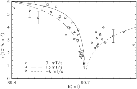
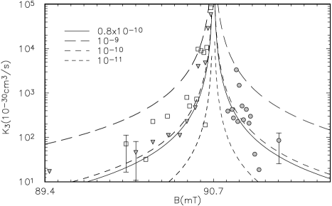
FIG. 1.: The surviving mean density vs. the stopping value of the magnetic field, calculated with the optimal value of the deactivation parameter $\gamma=0.8\times 10^{-11}$ cm${}^{3}/$s. The resonance was approached from below with two ramp speeds, 13 mT/s and 31 mT/s, or from above, with the ramp speed -6 mT/s. These are compared with the experimental results [4] (squares, triangles and circles) for several values of the ramp speed $dB/dt$ (in mT/s).

FIG. 2.: The 3-body rate coefficient ($K_{3}$) vs. the stopping value of the magnetic field, calculated with the optimal and other values of the deactivation parameter $\gamma$ (in units of cm³/s), on approaching the resonance from below or above. The calculated value of $K_{3}$ is independent of the ramp speed value. Other notations as in Fig. 1.

FIG. 3.: Ratio of surviving trap population $N$ to the initial one $N_{0}$ for the 85.3mT (853G) and 90.7mT (907G) resonances [parts (a) and (b), respectively] in the homogeneous-density approximation vs. $sn_{0}$ (where the parameter $s$ is defined by Eq. (84) and $n_{0}$ is the initial density). The curves show results of calculations carried out for different magnitudes of the parameters $\gamma$ and $\gamma_{m}$ (in units of cm³/s), without accounting for the excitation mechanism. The asymptotic analytical result Eq. (84) is given by the dotted line. The results of the MIT fast-sweep experiment (Ref. [4]) are shown for comparison.

FIG. 4.: Same as Fig. 7 but accounting for the excitation mechanism. The results of calculations without accounting for the excitation mechanism are given for comparison by the dotted line. In the part (b) the plot calculated for $\gamma=10^{-10}$cm${}^{3}/$s and different magnitudes of $\gamma_{m}$ are practically indistinguishable.

FIG. 5.: Time-dependence of the molecular condensate density in cm^-3 during fast passage through the 85.3mT (853G) and 90.7mT (907G) resonances [parts (a) and (b), respectively], calculated using the value of $\gamma=10^{-10}$cm${}^{3}/$s. The dashed and solid lines are calculated accounting for the combined effect of the two mechanisms (deactivation and excitation) for $sn_{0}=1$ and 5, respectively, and $\gamma_{m}=10^{-9}$cm${}^{3}/$s. The dotted and dash-dotted lines refer only to the deactivation mechanisms for $\gamma_{m}=0$ and $10^{-9}$cm${}^{3}/$s, respectively, and $sn_{0}=1$. The oscillations of the molecular density are faster for the lower value of $sn_{0}$.

FIG. 6.: Peak values of the molecular condensate density in cm^-3 attained during fast passage through the 85.3mT (853G) and 90.7mT (907G) resonances [parts (a) and (b), respectively] vs. $sn_{0}$ for various magnitudes of the parameter$s\gamma$ and $\gamma_{m}$ (see Caption of Fig. 7), calculated without accounting for the excitation mechanism.

FIG. 7.: Same as Fig. 7 but accounting for the excitation mechanism. The results of calculations without accounting for the excitation mechanism are given for comparison by the dotted line. In the part (b) the plot calculated for $\gamma=10^{-10}$cm${}^{3}/$s with $\gamma_{m}=0$ and $10^{-10}$ cm${}^{3}/$s are practically indistinguishable.

TABLE I.: Asymptotic conditions as consistency tests on solutions of Eq. (76)

	case	$\dot{n}$	$n$
a	$n\rightarrow$const	$\dot{n}\rightarrow 0$	$n\rightarrow$const
b	$n/t\rightarrow 0$	$\dot{n}\sim-6|g|^{2}\gamma n^{3}/\left(\mu\dot{B}t\right)^{2}$	$n\rightarrow\text{const}$
c	$n/t\rightarrow\infty$	$\dot{n}\sim-6|g|^{2}n/\left(\hbar^{2}\gamma\right)$	$n\sim\exp\left[-6|g|^{2}t/\left(\hbar^{2}\gamma\right)\right]$
d	$n/t\rightarrow$const	$\dot{n}\sim t$	$n\sim t^{2}$

REFERENCES

- [1] A. S. Parkins and D. F. Walls, Phys. Rep. 303, 1 (1998).
- [2] F. Dalfovo, S. Giorgini, L. P. Pitaevskii, and S. Stringari, Rev. Mod. Phys. 71, 463 (1999).
- [3] S. Inouye, M. R. Andrews, J. Stenger, H.-J. Miesner, D. M. Stamper-Kurn, and W. Ketterle, Nature 392, 151 (1998).
- [4] J. Stenger, S. Inouye, M. R. Andrews, H.-J. Miesner, D. M. Stamper-Kurn, and W. Ketterle, Phys. Rev. Lett. 82, 4569 (1999).
- [5] E. Tiesinga, B.J. Verhaar, and H.T.C. Stoof,Phys. Rev. A47, 4114 (1993); E. Tiesinga, A.J. Moerdijk, B.J. Verhaar, and H.T.C. Stoof, Phys. Rev. A46, R1167 (1992).
- [6] E. Timmermans, P. Tommasini,M. Hussein, and A. Kerman, Phys. Rep., 315, 199 (1999).
- [7] V. A. Yurovsky, A. Ben-Reuven, P. S. Julienne and C. J. Williams, in Cold atomic collisions: formation of cold molecules (Centre of Physics, Les Houches, France, 1999).
- [8] V. A. Yurovsky, A. Ben-Reuven, P. S. Julienne and C. J. Williams, Phys. Rev. A 60, R765 (1999).
- [9] F. A. van Abeelen, and B. J. Verhaar, Phys. Rev. Lett. 83, 1550 (1999).
- [10] F. H. Mies, P. S. Julienne, and E. Tiesinga, Phys. Rev. A 61, 022721 (2000).
- [11] R. C. Forrey, V. Kharchenko, N. Balakrishnan and A. Dalgarno, Phys. Rev. A 59, 2146 (1999).
- [12] V. A. Yurovsky, A. Ben-Reuven, P. S. Julienne, and Y. B. Band, J. Phys. B 32, 1845 (1999).
- [13] J.-P. Blaizot and G. Ripka, Quantum Theory of Finite Systems (MIT Press,Cambridge, MA, 1986).
- [14] M. Edwards, R. J. Dodd, C. W. Clark, and K. Burnett, J. Res. Natl. Inst. Stand. Technol. 101, 553 (1996).
- [15] G. S. Agarwal, Quantum statistical theories of spontaneous emission (Springer, Berlin, 1974).
- [16] L. P. Pitaevsky, Zh. Exp. Teor. Fiz. 40, 646 (1961) [Sov. Phys.-JETP 13, 451 (1961)]; E. P. Gross, Nuovo Simento 20, 454 (1961).
- [17] M.-O. Mewes, M. R. Andrews, N. J. van Druten, D. M. Kurn, D. S. Durfee, and W. Ketterle, Phys. Rev. Lett. 77, 416 (1996).
- [18] V. A. Yurovsky and A. Ben-Reuven, J. Phys. B 31,1 (1998).
- [19] P. S. Julienne and F. H. Mies, J. Opt. Soc. Am. B 6, 2257 (1989); P. S. Julienne, A. M. Smith, and K. Burnett, Adv. At. Mol. Opt. Phys. 30, 141 (1993).
- [20] M. Shapiro and P. Brumer, J. Chem. Soc., Faraday Trans. 93, 1263 (1997).
- [21] R. J. Gordon and S. A. Rice, Annu. Rev. Phys. Chem. 48, 601 (1997).
- [22] K. Bergmann, H. Theuer, and B. W. Shore, Rev. Mod. Phys. 70, 1003 (1998).