Abstract

A model of a strongly correlated electron liquid based on the fermion condensation (FC) is extended to high-temperature superconductors. Within our model, the appearance of FC presents a boundary separating the region of a strongly interacting electron liquid from the region of a strongly correlated electron liquid. We study the superconductivity of a strongly correlated liquid and show that under certain conditions, the superconductivity vanishes at temperatures $T>T_{c}\simeq T_{node}$, with the superconducting gap being smoothly transformed into a pseudogap. As the result, the pseudogap occupies only a part of the Fermi surface. The gapped area shrinks with increasing the temperature and vanishes at $T=T^{*}$. The single-particle excitation width is also studied. The quasiparticle dispersion in systems with FC can be represented by two straight lines characterized by the respective effective masses $M^{*}_{FC}$ and $M^{*}_{L}$, and intersecting near the binding energy that is of the order of the superconducting gap. It is argued that this strong change of the quasiparticle dispersion at the binding can be enhanced in underdoped samples because of strengthening the FC influence. The FC phase transition in the presence of the superconductivity is examined, and it is shown that this phase transition can be considered as kinetic energy driven.

PACS numbers: 71.27.+a, 74.20.Fg, 74.25.Jb

1 Introduction

Unusual properties of the normal state of high-temperature superconductors have been attracting attention for a long time. In describing these properties, which are well beyond the standard Fermi liquid theory, the notion of a strongly correlated liquid has emerged (see e.g. [1, 2]). Later on, angle-resolved photoemission studies revealed unusual properties observed in underdoped samples, with the leading edge gap discovered up to the temperature $T^{*}>T_{c}$. This behavior is interpreted as coming from the pseudogap formation; it was observed in a number of underdoped compounds such as YBa₂Cu₃O_6+x, Bi₂Sr₂CaCu₂O_8+δ, etc. As $T$ increases above $T^{*}$, the pseudogap closes, leading to a large Fermi surface and an extremely flat dispersion in electronic spectra, which is called the extended Van Hove singularity $[3-7]$. Thereupon recent discovery of a new energy scale for quasiparticle dispersion in Bi₂Sr₂CaCu₂O_8+δ in the superconducting and in normal states [8, 9] have brought new insight to the physics of high temperature superconductors (HTS), imposing serious constraints upon the theory of HTS. The newly discovered additional energy scale manifests itself as a break in the quasiparticle dispersion near $(50-70)\,$meV, which results in a drastic change of the quasiparticle velocity [8, 9, 10]. Such a behavior is definitely different from what one could expect in a normal Fermi liquid.

A correlated liquid can be described in conventional terms, assuming that the correlated regime is related with the noninteracting Fermi gas by adiabatic continuity. This is done in the well-known Landau theory of the normal Fermi liquid, but the question arising at this point is whether this is possible. Most likely, the answer is negative. To tackle the above-mentioned problems, we consider a model where a strongly correlated liquid is separated from the conventional Fermi liquid by a phase transition related to the onset of the FC [11, 12]. The purpose of our paper is to show that without any adjustable parameters, a number of fundamental problems of strongly correlated systems are naturally explained within the model. The paper is organized as follows. In Sec. 2, we consider the general features of Fermi systems with the FC. In Sec. 3, we show that the pseudogap behavior can be understood within the standard BCS superconductivity mechanism provided the appearance of FC is taken into account. In Sec. 4, we analyze the condensation energy that is liberated when the system in question undergoes the superconducting phase transition superimposing on the FC phase transition. In Sec. 5, we describe the quasiparticle dispersion and lineshape. Finally, in Sec. 6, we summarize our main results.

2 The main features of liquids with FC

We first consider the key points of the FC theory. The FC is related to a new class of solutions of the Fermi liquid theory equation [13]

$$\frac{\delta(F-\mu N)}{\delta n(p,T)}=\varepsilon(p,T)-\mu(T)-T\ln\frac{1-n(p,T)}{n(p,T)}=0$$ (1)

for the quasiparticle distribution function $n(p,T)$ depending on the momentum $p$ and the temperature $T$. Here $F$ is the free energy, $\mu$ is the chemical potential, and $\varepsilon(p,T)=\delta E/\delta n(p,T)$ is the quasiparticle energy, which is a functional of $n(p,T)$ just like the energy $E$ and the other thermodynamic functions. Equation (1) is usually represented as the Fermi-Dirac distribution

$$n(p,T)=\left\{1+\exp\left[\frac{(\varepsilon(p,T)-\mu)}{T}\right]\right\}^{-1}.$$ (2)

In a homogeneous matter and at $T=0$, one obtains from Eq. (2) the standard solution $n_{F}(p,T=0)=\theta(p_{F}-p)$, with $\varepsilon(p\simeq p_{F})-\mu=p_{F}(p-p_{F})/M^{*}_{L}$, where $p_{F}$ is the Fermi momentum and $M^{*}_{L}$ is the commonly used effective mass [13],

$$\frac{1}{M^{*}_{L}}=\frac{1}{p}\frac{d\varepsilon(p,T=0)}{dp}|_{p=p_{F}}.$$ (3)

It is assumed to be positive and finite at the Fermi momentum $p_{F}$. This implies the $T$-dependent corrections to $M^{*}_{L}$, the quasiparticle energy $\varepsilon(p)$, and the other quantities start with $T^{2}$-terms.

But this solution of Eq. (1) is not the only one possible. There exist “anomalous” solutions of Eq. (1) associated with the so-called fermion condensation [11, 14, 15]. Being continuous and satisfying the inequality $0<n(p)<1$ within some region in $p$, such a solution $n(p)$ admits a finite limit for the logarithm in Eq. (1) as $T\rightarrow 0$, yielding

$$\varepsilon(p)=\frac{\delta E[n(p)]}{\delta n(p)}=\mu,\>p_{i}\leq p\leq p_{f}.$$ (4)

Equation (4) is used in searching the minimum value of $E$ as a functional of $n(p)$ under the assumption that a strong rearrangement of the single-particle spectrum can occur. We see from Eq. (4) that the occupation numbers $n(p)$ become variational parameters: the solution $n(p)$ exists if the energy $E$ is decreased by alteration of the occupation numbers. Thus, within the region $p_{i}<p<p_{f}$, the solution $n(p)$ deviates from the Fermi step function $n_{F}(p)$ such that the energy $\varepsilon(p)$ stays constant, while $n(p)$ coincides with $n_{F}(p)$ outside this region. As a result, the standard Kohn — Sham scheme for the single-particle equations is no longer valid beyond the FC phase transition point [16]. This behavior of systems with the FC is clearly different from what one expects from the well known local density calculations; therefore, these calculations are not applicable to systems with the FC. On the other hand, the quasiparticle formalism is applicable to this problem, because as we see in what follows, the damping of single-particle excitations is not large compared to their energy [15]. It is also seen from Eq. (4) that a system with the FC has a well-defined Fermi surface.

It follows from Eq. (1) that at low $T$, new solutions within the interval occupied by the fermion condensate have the spectrum $\varepsilon(p,T)$ that is linear in T [15, 17],

$$\varepsilon(p,T)-\mu(T)\simeq\frac{(p-p_{F})p_{F}}{M^{*}_{FC}}\simeq T(1-2n(p))\ll T_{f}.$$ (5)

Here $T_{f}$ is the quasi-FC phase transition temperature above which FC effects become insignificant [15],

$$\frac{T_{f}}{\varepsilon_{F}}\sim\frac{p_{f}^{2}-p_{i}^{2}}{2M\varepsilon_{F}}\sim\frac{\Omega_{FC}}{\Omega_{F}},$$ (6)

where $M$ is the bare electron mass, $\Omega_{FC}$ is the condensate volume, $\varepsilon_{F}$ is the Fermi energy, and $\Omega_{F}$ is the volume of the Fermi sphere. One can imagine that the dispersionless plateau $\varepsilon(p)=\mu$ given by Eq. (4) is slightly tilted counter-clockwise about $\mu$ and rounded off at the end points. If $T\ll T_{f}$, it follows from Eqs. (1) and (5) that the effective mass $M^{*}_{FC}$ related to the FC is temperature dependent

$$\frac{M^{*}_{FC}}{M}\sim\frac{N(0)}{N_{0}(0)}\sim\frac{T_{f}}{T},$$ (7)

where $N_{0}(0)$ is the density of states of the noninteracting electron gas, and $N(0)$ is the density of states at the Fermi level. We note that outside the FC region, the single-particle spectrum is not distinctly affected by temperature, being determined by the effective mass $M^{*}_{L}$ given by Eq. (3), which is now evaluated at $p\leq p_{i}$. Thus, we are led to the conclusion that systems with a FC must be characterized by two effective masses: $M^{*}_{FC}$ related to the single particle spectrum of a low-energy scale and $M^{*}_{L}$ related to the spectrum of a higher energy scale. The existence of these two effective masses can be observed as a break in the quasiparticle dispersion. This break is observed at temperatures $T\ll T_{f}$, and also when the superconducting state is superimposed on the FC state. In the former case, the occupation numbers over the area occupied by the fermion condensate are slightly disturbed by the pairing correlations such that the effective mass $M^{*}_{FC}$ becomes large but finite. We remark that at comparatively low temperatures, the FC and superconductivity go together because of the remarkable peculiarities of the FC phase transition. This transition is related to a spontaneous gauge symmetry breaking: the superconductivity order parameter $\kappa(p)=\sqrt{n(p)[1-n(p)]}$ has a nonzero value over the region occupied by the fermion condensate, while the gap $\Delta$ can vanish [15, 16].

It is seen from Eq. (4) that at the FC phase transition point $p_{f}\to p_{i}\to p_{F}$, while the effective mass and the density of states tend to the infinity as follows from Eqs. (4) and (7). One can conclude that the beginning of the FC phase transition is related to the absolute growth of $M^{*}_{FC}$. The onset of the charge density-wave instability in an electron system, which occurs as soon as the effective electron-electron interaction constant $r_{s}$ reaches its critical value $r_{cdw}$, must be preceded by the unbounded growth of the effective mass [18]. For a simple electron liquid, the effective constant is proportional to the dimensionless average distance $r_{s}\sim r_{0}/a_{B}$ between particles of the system in question, with $r_{0}$ being the average distance and $a_{B}$ the Bohr radius. The physical reason for this growth is the contribution of the virtual charge density fluctuations to the effective mass. The excitation energy of these fluctuations becomes very small if $r_{s}\simeq r_{cdw}$. Thus, a FC can occur when $r_{s}\sim r_{cdw}$. The standard Fermi liquid behavior can therefore be broken by strong charge fluctuations when the insulator regime is approached in a continuous fashion. We recall that the charge-density wave instability occurs in three-dimensional [19] and two-dimensional (2D) electron liquids [20] at a sufficiently high $r_{s}$. As soon as $r_{s}$ reaches its critical value $r_{FC}<r_{cdw}$, the FC phase transition occurs. Thereafter, the condensate volume is proportional to $r_{s}-r_{FC}$ and also $T_{f}/\varepsilon_{F}\sim r_{s}-r_{FC}$ [15, 18]. In fact, the effective coupling constant $r_{s}$ increases with decreasing doping. It is assumed that both $T_{f}$ and condensate volume $\Omega_{FC}$ build up with decreasing doping. The FC then serves as a stimulating source of new phase transitions lifting the degeneracy of the spectrum. The FC can produce, for instance, the spin density wave (SDW) phase transition or the antiferromagnetic one, thereby promoting a variety of the system properties. We note that the SDW phase transition, the antiferromagnetic transition, and the charge density one also depend on $r_{s}$ and occur at a sufficiently large value of $r_{s}$ even if the FC is absent. The superconducting phase transition is also aided by the FC. We analyze the situation where the superconductivity wins the competition with the other phase transitions up to a temperature $T_{c}$. Above the temperature $T^{*}\ll T_{f}$ the system under consideration is in its anomalous normal state, Eq. (7) is valid, and one can observe smooth non-dispersive segments of the spectra at the Fermi surface [6].

3 Superconductivity in the presence of FC

We focus our attention on investigating the pseudogap that is formed above $T_{c}$ in underdoped (UD) high-temperature superconductors $[4-8]$. As we see in what follows, the existence of the pseudogap is closely allied with the presence of the FC characterized by a sufficiently high temperature $T_{f}$ given by Eq. (6). Thus, the pseudogap is peculiar to UD samples, while optimally doped (OP) and overdoped (OD) samples may not exhibit this feature. We consider a 2D liquid on a simple square lattice that has a superconducting state with the d-wave symmetry of the order parameter $\kappa$. We assume that the long-range component $V_{lr}({\bf q})$ of the particle-particle interaction $V_{pp}({\bf q})$ is repulsive and has the radius $q_{lr}$ in the momentum space such that $p_{F}/q_{lr}\leq 1$. The short-range component $V_{sr}({\bf q})$ is relatively large and attractive, with its radius $p_{F}/q_{sr}\gg 1$. In agreement with the d-symmetry requirements the low temperature gap $\Delta$ is then given by the expression [21, 22, 23]

$$\Delta(\phi)=2\kappa(\phi)E(\phi)\simeq\Delta_{1}\cos 2\phi=\Delta_{1}(x^{2}-y^{2}),$$

where $E(\phi)=\sqrt{\varepsilon^{2}(\phi)+\Delta^{2}(\phi)}$ and $\Delta_{1}$ is the maximal gap. At finite temperatures, the equation for the gap can be written as

$$\Delta(p,\phi)=-\int_{0}^{2\pi}\int V_{pp}(p,\phi,p_{1},\phi_{1})\kappa(p_{1},\phi_{1})\tanh{E(p_{1},\phi_{1})\over 2T}\frac{p_{1}dp_{1}d\phi_{1}}{4\pi^{2}},$$ (8)

where $p$ is the absolute value of the momentum and $\phi$ is the angle. It is also assumed that the FC arises near the van Hove singularities, leading to a large density of states at these points in accordance with Eq. (7). We note that the different FC areas overlap only slightly [17]. $\Delta(\phi)$ obeys the following equation that is determined by the chosen interaction $V_{pp}$

$$\Delta({\pi\over 4}+\phi)=-\Delta({\pi\over 4}-\phi).$$ (9)

It vanishes at $\pi/4$ and can therefore be expanded in the Taylor series around $\pi/4$, with $p\approx p_{F}$:

$$\Delta(p,\theta)=\theta a-\theta^{3}b+...,$$ (10)

where $\theta=\phi-{\pi\over 4}$. Hereafter, we consider solutions of Eq. (8) on the interval $0<\theta<\pi/4$. We transform Eq. (8) by setting $p\approx p_{F}$ and separating the contribution $I_{lr}$ coming from $V_{lr}$, with the contribution related to $V_{sr}$ denoted by $I_{sr}$. At small angles, $I_{lr}$ can be approximated in accordance with (10) by $I_{lr}=\theta A+\theta^{3}B$, with the parameters $A$ and $B$ independent of $T$ if $T\leq T^{*}\ll T_{f}$, because they are defined by the integral over the regions occupied by the FC. This theoretical observation is consistent with the experimental results showing that $\Delta_{1}$ is essentially $T$-independent at the temperatures $T<T^{*}$ [6]. The coefficients of the expansion of $I_{sr}$ in powers of $\theta$ depend on $T$. It is therefore more convenient to use the integral representation for $I_{sr}$ following from (8). We, thus, have

$$\Delta(\theta)=I_{sr}+I_{lr}=-\int_{0}^{2\pi}\int V_{sr}(\theta,p_{1},\phi_{1})\kappa(p_{1},\phi_{1})\tanh{E(p_{1},\phi_{1})\over 2T}\frac{p_{1}dp_{1}d\phi_{1}}{4\pi^{2}}+\theta A+\theta^{3}B.$$ (11)

In Eq. (11), the variable $p$ was omitted since $p\approx p_{F}$. It is seen from this equation that the FC produces the free term $\theta A+\theta^{3}B$. In what follows, we show that at $T\geq T_{node}$, the solution of Eq. (11) has the second node at $\theta_{c}(T)$ in the vicinity of the first node at $\pi/4$. We also demonstrate that the temperature $T_{node}$ has the meaning of the temperature $T_{c}$ at which the superconductivity vanishes. To show this, we simplify Eq. (11) to an algebraic equation. We have $I_{sr}\sim(V_{0}/T)\theta$ because $\tanh(E/2T)\approx E/2T$ for $E\ll T$ and $T\approx T_{node}$, as is the case in the vicinity of the gap node at $\theta=0$. The integration in Eq. (11) runs over a small area located at the gap node because of the small radius of $V_{sr}$. Dividing both parts of Eq. (11) by $\kappa(\theta)$, we obtain

$$E(\theta)=-({V_{0}\over T}-A_{1}-\theta^{2}B_{1})|\theta|,$$ (12)

where $A_{1}$ and $B_{1}$ are new constants and $V_{0}\sim V_{sr}(0)$ is a constant. Imposing the condition that Eq. (8) has the only solution $\Delta\equiv 0$ when $V_{sr}=0$, we see that $A_{1}$ is negative and $B_{1}$ is positive. The factor in the brackets on the right-hand side of Eq. (12) changes its sign at some temperature $T_{node}\approx V_{0}/A_{1}$; on the other hand, the excitation energy must be $E(\theta)>0$. Therefore, we have two possibilities [24, 25]. The first follows from the assumption that $\Delta(\theta)\equiv 0$ if $\theta$ belongs to the interval $\Omega_{n}$ $[0<\theta<\theta_{c}]$. In this case, for $T>T_{node}$ we must solve Eq. (8) with the condition

$$\Delta(\theta)\equiv 0,\,\,\,{\rm if:}\,\,0<\theta<\theta_{c};\,\,\,T_{node}<T.$$

This resembles Eq. (4) with the parameter $\mu$ being equal to zero. The similarity is not coincidental, because we are searching for new solutions in both cases. Such solutions do exist because the points $\theta=0$ and $\theta=\theta_{c}$ represent the branching points of the solutions. The second possibility can occur if the above solution does not lead to a minimum value of the free energy. Because the excitation energy must be positive for a stable state, the sign of $\Delta$ must be reversed at the point $\theta=\theta_{c}$. Then the gap $\Delta(\theta)$ has the same sign within the interval $\Omega_{n}$ and changes its sign once more at the point $\theta=0$, with $\Delta(\theta_{c})=\Delta(0)=0$. Thus, we conclude that the gap $\Delta$ possesses new nodes at $T>T_{node}$ [25], see Fig. 1. It can be seen from Eq. (12) that the angle $\theta_{c}$ is related to $T>T_{node}$ by

$$T\approx\frac{V_{0}}{(A_{1}+B_{1}\theta_{c}^{2})}.$$ (13)

It follows from the above consideration and Eq. (12) that even below $T_{node}$, the order parameter $\Delta$ cannot be approximated by a simple d-wave form; a more sophisticated expression must be used to fit the flattening of the gap $\Delta$ around the node. The following expression can be used for this purpose,

$$\Delta(\phi)=\Delta_{1}[B\cos(2\phi)+(1-B)\cos(6\phi)].$$ (14)

Here $0<B<1$ in accordance with the experimental results [7] and the term involving $\cos(6\phi)$ is the next compatible with the d-symmetry of the gap. It also follows from Eq. (12) that the parameter $B$ is a decreasing function of the temperature. At the temperatures $T>T_{node}$, the value of $(1-B)$ is sufficiently large to produce new nodes of $\Delta$ given by Eq. (14).

As an example of the solutions of Eqs. (8) and (11), we show, in Fig. 1 the gap $\Delta(\phi)$ calculated at three different temperatures $0.9\,T_{node}$, $T_{node}$, and $1.2\,T_{node}$. An important difference between curves (b) and (a) is the flattening of curve (b) at the nodes localized within the region $\Omega_{n}$ containing the interval $-\theta_{c}\leq\theta\leq\theta_{c}.$ As seen from Fig. 1, the flattening occurs as the result of the new nodes restricting the area $\Omega_{n}$. It is also seen from Fig. 1 that the gap $\Delta$ is extremely small over the range $\Omega_{n}$.

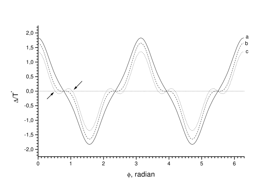
Figure 1: The gap $\Delta$ as a function of $\phi$ calculated at three different temperatures expressed in terms of $T_{node}\simeq T_{c}$, while $\Delta$ is presented in terms of $T^{*}$. Curve (a), solid line, shows the gap calculated at temperature $0.9T_{node}$. In curve (b), dashed line, the gap is given at $T_{node}$. Note the important difference in curve (b) compared with curve (a) due to a flattening of the curve (b) over the region $\Omega_{n}$. Calculated $\Delta(\phi)$ at $1.2T_{node}$ is shown by curve (c), dotted line. The arrows indicate the two nodes restricting area $\Omega_{n}$ and emerged at $T_{node}$.

It was recently shown in a number of papers (see, e.g., [26, 27]) that there exists an interplay between the magnetism and the superconductivity order parameters, leading to the damping of the magnetism order parameter below $T_{c}$. Conversely, one can anticipate the damping of the superconductivity order parameter by magnetism. Thus, we conclude that the gap in the range $\Omega_{n}$ can be destroyed by strong antiferromagnetic correlations (or by spin density waves) existing in underdoped superconductors [28, 29]. It is believed that impurities can easily destroy $\Delta$ in the considered area. As a result, one is led to the conclusion that $T_{c}\simeq T_{node}$, with the exact value of $T_{c}$ defined by the competition between the antiferromagnetic correlations (or spin density waves) and the superconducting correlations over the range $\Omega_{n}$.

We now consider the possibility for two quite different properties, the superconductivity and static spin density wave (SDW), to coexist. We start by briefly outlining the main features of the SDW [30]. A simple example is given by the linear SDW, with the net spin polarization ${\bf P}(\bf r)$

$${\bf P}({\bf r})=P_{0}{\bf e}\cos(\hat{Qx}),$$ (15)

where $\hat{Qx}$ is the angle between the vectors ${\bf Q}$ and ${\bf x}$. For convenience, the direction of the SDW is taken along the ${\bf x}$ axis, and ${\bf e}$ is the unit polarization vector, which in general can have any orientation with respect to ${\bf Q}$. In contrast to the superconductivity, SDW can occupy only a part of the Fermi sphere with the volume $\delta S\simeq p_{F}\delta\phi\delta k$, where $\delta\phi$ is the Fermi surface angle and $\delta k$ is the “penetration depth” of the SDW into the Fermi sphere. At $T=0$, the energy gain $\delta W$ due to the onset of SDW is given by

$$\delta W\simeq g^{2}N(0)\delta\phi,$$ (16)

where $g$ is the SDW gap determined by the formula [30]

$$g\simeq\frac{p_{F}\delta k}{N(0)}\exp(-\frac{4}{N(0)\gamma_{0}\delta\phi}),$$ (17)

where $\gamma_{0}$ is the coupling constant. As seen from Eq. (8), the variation of the gap within some area produces a variation of the gap over the entire occupied area with the same order of magnitude. Therefore, elimination of $\Delta$ over a segment $\delta\phi$ requires the energy $\delta E_{1}\sim N(0)\Delta^{2}(\phi)$. We conclude that at $T<T_{node}$, the destruction of the gap on the interval $\delta\phi$ eliminates $\Delta$ over the entire region, because $\delta E_{1}$ is comparable with the gain $\delta E$ due to the superconducting state. A different situation occurs at the temperatures $T>T_{node}$, when $\Delta$ is extremely small in $\Omega_{n}$ and the corresponding destruction energy satisfies inequality $\delta E_{1}\ll\delta E$. Equations (16) and (17) are very similar to the corresponding BCS equations and this similarity also remains at finite temperatures [30]. Thus, the gain $\delta W$ and the gap $g$ vary with the temperature similarly to the superconducting gain $\delta E$ and the gap $\Delta$. We also assume that the SDW transition temperature $T_{n}$ is sufficiently high, namely, $T_{n}\geq T_{c}$. We then come to the conclusion that $\delta E_{1}<\delta W$, and the region $\Omega_{n}$ is therefore occupied by the SDW at temperatures $T\geq T_{node}$, resulting in the destruction of the superconductivity [24, 25]. We note that the Fermi surface angle $\delta\phi$ must be sufficiently large, because the gap $g$ depends exponentially on $\delta\phi$ in accordance with Eq. (17). On the other hand, because we are dealing with SDW, we have $\delta\phi/\pi\sim 10^{-2}$ [30]. We thus conclude that a strong variation of the superconductivity characteristics may be observed in the vicinity of $T_{node}$.

It follows from the above considerations that $\Delta(\theta)$ can be destroyed only locally within the region $\Omega_{n}$ because of the different reasons. It also follows that $T_{node}$ is the temperature at which the superconductivity vanishes, that is, $T_{c}\simeq T_{node}$. As to the gap at $T>T_{c}$, or more precisely, the pseudogap, it persists outside the $\Omega_{n}$ region. In accordance with [4, 7], we see that the superconducting gap $\Delta(\theta)$ smoothly transforms into the pseudogap at $T>T_{c}$. We can therefore expect a dramatic reduction in the difference between the free energy of the normal and the superconducting state at $T=T_{c}$ (the so-called condensation energy, which we consider in some detail in the next section). It can then be concluded that the temperature $T^{*}$ has the physical meaning of the BCS transition temperature between the state with the order parameter $\kappa\neq 0$ and the normal state. Because $T_{c}\simeq V_{0}/A_{1}$, we find from Eq. (13) that $\theta_{c}\sim\sqrt{(T-T_{c})/T_{c}}$. This result is in harmony with our calculations of the function $\theta_{c}([T-T_{c}]/T_{c})$ plotted in Fig. 2. Thus, we conclude that the pseudogap “dies out” in UD samples as the temperature $T^{*}$ is approached. Quite naturally, one has to recognize that $\Delta_{1}$ must scale with $T^{*}$.

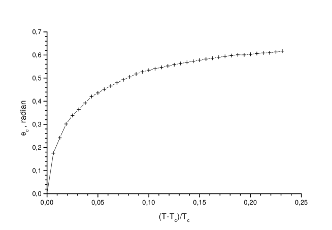
Figure 2: Calculated angle $\theta_{c}$, pulling apart the two nodes, as a function of $(T-T_{c})/T_{c}$.

A few remarks are in order at this point. On the basis of the previous consideration, we conclude that the BCS approach is fruitful in considering OD, OP, and UD samples in the weak coupling regime. With more underdoping, the antiferromagnetic correlations become stronger, breaking down the gap over the range $\Omega_{n}$ at lower temperatures. Thus, one observes the decrease of $T_{c}$ with the decrease of doping. On the other hand, the condensate volume $\Omega_{FC}$ becomes larger with the decrease of doping, leading to increase of the gap $\Delta_{1}$ which is proportional to the volume and interaction $V_{pp}$ [11]. Consequently, the temperature $T^{*}$ becomes higher with decreasing doping. All these results are in agreement with the experimental findings [4, 7]. A peak was observed at 41 meV$\simeq 2\Delta_{1}$ in inelastic neutron scattering from single crystals of the OD, OP, and UD samples YBa₂Cu₃O_6+x and Bi₂Sr₂CaCu₂O_8+δ at temperatures below $T_{c}$, while a broad maximum above $T_{c}$ exists in underdoped samples only [31, 32]. The explanation of this peak given in [33] was based on the ideas of the BCS theory. From the above discussion, it appears that the same explanation holds for the broad maximum in underdoped samples above $T_{c}$ because the physics of the process is essentially the same.

4 Condensation energy

We now consider the energy gain or condensation energy $E_{cond}$ liberated when the system in question undergoes the superconducting phase transition involved in the FC phase transition. We set $T=0$ for simplicity. The energy $E_{cond}$ can be schematically broken into two parts related to the kinetic and the potential energy. The condensation energy was considered in [34], where it was argued that the main contribution to the condensation energy comes from the kinetic energy, i.e., the superconducting phase transition of high-temperature superconductors is kinetic energy driven. Here, we give a possible interpretation of the situation. It is known [35] that in the superconducting phase transition, the positive contribution comes from the potential energy, while the gain in the kinetic energy is negative. In the other words, the superconducting phase transition is driven by the gain in the potential energy. This result is rather obvious because the ground state energy $E_{gs}$ is given by

$$E_{gs}[\kappa({\bf p})]=E[n({\bf p})]+E_{sc}[\kappa({\bf p})],$$ (18)

with the occupation numbers $n({\bf p})$ determined by $\kappa({\bf p})=\sqrt{n({\bf p})[1-n({\bf p})]}$. The second term $E_{sc}[\kappa({\bf p})]$ on the right-hand side of Eq. (18) is defined by the superconducting contribution, which in the simplest case is of the form

$$E_{sc}[\kappa({\bf p})]=g_{2}\int V_{pp}({\bf p}_{1},{\bf p}_{2})\kappa({\bf p}_{1})\kappa({\bf p}_{2})\frac{d{\bf p}_{1}d{\bf p}_{2}}{(2\pi)^{4}}.$$ (19)

The first term $E[n({\bf p})]$ can be taken as

$$E[n({\bf p})]=\int\frac{p^{2}}{2M}n({\bf p})\frac{d{\bf p}}{4\pi^{2}}+\frac{g_{1}}{2}\int V({\bf p}_{1},{\bf p}_{2})n({\bf p}_{1})n({\bf p}_{2})\frac{d{\bf p}_{1}d{\bf p}_{2}}{(2\pi)^{4}},$$ (20)

with the second integral playing the role of the exchange-correlation contribution to the ground state energy. If the effective mass $M^{*}_{L}$ given by Eq. (3) is positive and finite, $E[n({\bf p})]$ reaches its minimum at $n(p)=n_{F}(p)$ and increases with the deviation of $n(p)$ from the Fermi distribution, as it occurs in the presence of superconducting correlations. Thus, the standard situation is that the superconducting phase transition is driven by a decrease of the potential energy [35]. The situation can be different if the system undergoes the FC phase transition. To see this we temporarily assume that $g_{2}\to 0$ and rewrite Eq. (20) as

$$E[n({\bf p})]=\int\varepsilon({\bf p})n({\bf p})\frac{d{\bf p}}{4\pi^{2}}-\frac{g_{1}}{2}\int V({\bf p}_{1},{\bf p}_{2})n({\bf p}_{1})n({\bf p}_{2})\frac{d{\bf p}_{1}d{\bf p}_{2}}{(2\pi)^{4}},$$ (21)

with the single particle energy

$$\varepsilon({\bf p})=\frac{\delta E[n({\bf p})]}{\delta n({\bf p})}.$$ (22)

The energy $E[n({\bf p})]$ can be lowered by alteration of $n({\bf p})$ if Eq. (4) has solutions. As the result, we can write the inequality [11]

$$E_{cond}=E_{N}-E_{FC}\geq\int\left(\varepsilon({\bf p})-\mu\right)\delta n({\bf p})\frac{d{\bf p}}{4\pi^{2}}\geq 0,$$ (23)

with $E_{N}$ being the energy of system in its normal state, $E_{FC}$ the energy with FC, and the integral taken over the region occupied by FC. The chemical potential $\mu$ preserves the conservation of the particle number under the variation $\delta n({\bf p})$. We assume that the kinetic energy is given by the first term on the right-hand side of Eq. (21). It then follows from Eq. (23) that the kinetic energy can be lowered, and this lowering is driven by the FC phase transition. It is instructive to illustrate this by a simple example. We take $V({\bf p}_{1},{\bf p}_{2})=g_{1}\delta({\bf p}_{1}-{\bf p}_{2})$, then $E_{cond}$ given by Eq. (23) becomes

$$E_{cond}=\int\left(\varepsilon_{0}({\bf p})n_{F}(p)-\varepsilon({\bf p})n(p)\right)\frac{d{\bf p}}{4\pi^{2}}+\frac{g_{1}}{2}\int\left(n^{2}(p)-n_{F}^{2}(p)\right)\frac{d{\bf p}}{4\pi^{2}},$$ (24)

with $\varepsilon_{0}({\bf p})$ being the single particle energy of the normal ground state. It is easily verified that the second term on the right-hand side of Eq. (24), which is related to the potential energy gain, is negative. This term can be written as

$$\frac{g_{1}}{2}\int\left(n^{2}(p)-n_{F}^{2}(p)\right)\frac{d{\bf p}}{4\pi^{2}}=\frac{g_{1}}{2}\int\left(n(p)-n_{F}(p)\right)\left(n(p)+n_{F}(p)\right)\frac{d{\bf p}}{4\pi^{2}}.$$

Observing that

$$\int\left(n(p)-n_{F}(p)\right)\frac{d{\bf p}}{4\pi^{2}}=0$$

because of the particle number conservation and taking into account that

$$(n(p)+n_{F}(p))|_{p\leq p_{F}}>(n(p)+n_{F}(p))|_{p_{F}\leq p},$$

we arrive at the conclusion. The first term is positive because of inequality (23). Thus, we are led to the conclusion that the FC phase transition can be considered as driven by the kinetic energy. We now let the coupling constant $g_{2}$ be small, then the gap $\Delta$ is proportional to $g_{2}$ [11]. The optimum values of the occupation numbers given by Eq. (4) are disturbed, leading to an increase of the energy $E[n({\bf p})]$. The positive gain in the potential energy given by Eq. (19) is driving the formation of the superconducting ground state. Because the coupling constant $g_{2}$ is sufficiently small, the structure of the system ground state is defined by the FC, and the superconducting state is a “shadow” of the FC under these conditions [15]. Then, the main contribution to $E_{cond}$ comes from the FC phase transition, and the complex transition (FC plus superconductivity) is kinetic energy driven [36]. On the other hand, in the case where FC is weak compared to the superconductivity (or is absent), we are dealing with a pure superconducting phase transition, which is obviously potential energy driven.

5 Quasiparticle dispersion and lineshape

We now discuss the origin of two effective masses $M^{*}_{L}$ and $M^{*}_{FC}$ occurring in the superconducting state and leading to a nontrivial quasiparticle dispersion and a change of the quasiparticle velocity. As we see in what follows, our results are in a reasonably good agreement with the experimentally deduced data [10, 8, 9]. For simplicity we set $T=0$. Varying $E_{gs}$ given by Eq. (18) with respect to $\alpha_{\bf p}$, we find

$$\frac{E_{gs}[\alpha_{\bf p}]}{\delta\alpha_{\bf p}}=(\varepsilon({\bf p})-\mu)\tanh(2\alpha_{\bf p})+\Delta({\bf p})=0,$$ (25)

with $n({\bf p})=\cos^{2}(\alpha_{\bf p})$, $\kappa({\bf p})=\sin(\alpha_{\bf p})\cos(\alpha_{\bf p})$, and $\varepsilon({\bf p})$ defined by Eq. (22). As $g_{2}\to 0$, we have that $\Delta({\bf p})\to 0$, and Eq. (25) becomes

$$(\varepsilon({\bf p})-\mu)\tanh(2\alpha_{\bf p})=0.$$ (26)

Equation (26) requires that

$$\varepsilon({\bf p})-\mu=0,\,\,\,\,{\mathrm{if}}\,\,\,\tanh(2\alpha_{\bf p})\neq 0\,\,\,\,(0<n({\bf p})<1),$$ (27)

which leads to the FC solutions defined by Eq. (4) [16, 25]. As soon as the coupling constant $g_{2}$ becomes finite but small, such that $g_{2}/g_{1}\ll 1$, the plateau $\varepsilon({\bf p})-\mu=0$ is slightly tilted and rounded off at the end points. This implies that

$$\varepsilon({\bf p})-\mu\sim\Delta_{1},$$ (28)

which allows us to estimate the effective mass as

$$\frac{M^{*}_{FC}}{M}\sim\frac{T_{f}}{\Delta_{1}}.$$ (29)

Outside the condensate area, the quasiparticle dispersion is determined by the effective mass $M^{*}_{L}$ given by Eq. (3). We note that calculations in the context of a simple model support the above consideration [15]. In that case, putting $V({\bf p}_{1},{\bf p}_{2})=\delta({\bf p}_{1},{\bf p}_{2})$ and $V_{pp}({\bf p}_{1},{\bf p}_{2})=\delta({\bf p}_{1},{\bf p}_{2})$ in Eqs. (19) and (20) and carrying out direct calculations, we obtain at $T=0$

$$E_{0}=\varepsilon(p_{f})-\varepsilon(p_{i})\simeq\frac{(p_{f}-p_{i})p_{F}}{M^{*}_{FC}}\simeq 2\Delta_{1}.$$ (30)

On the other hand, at $T\geq T_{c}$, taking into account that $n(p_{i})\simeq 1$ and $n(p_{f})\simeq 0$, we obtain from Eq. (5) with the same accuracy,

$$E_{0}\simeq\frac{(p_{f}-p_{i})p_{F}}{M^{*}_{FC}}\simeq 2T.$$ (31)

Equations (30) and (31) allow us to estimate the effective mass $M^{*}_{FC}$ related to the region occupied by the FC at temperatures $T\ll T_{f}$. Outside the region, the effective mass is $M^{*}_{L}$. When Eqs. (28) and (29) are compared with Eqs. (5) and (7), it is apparent that the gap $\Delta_{1}$ plays the role of the effective temperature that defines the slope of the plateau. On the other hand, at $T=T_{c}$ in OD or OP samples, the gap vanishes and Eqs. (5) and (31) define the quasiparticle dispersion and the effective mass. Taking into account that $\Delta_{1}\sim T_{c}$, we are led to the conclusion that Eqs. (28) and (29) derived at $T=0$ match Eqs. (5) and (7) at $T_{c}$. Thus, Eqs. (28) and (29) are approximately valid over the range $0\leq T\leq T_{c}$. It follows from Eq. (30) that at $T\leq T_{c}$, the quasiparticle dispersion can be presented with two straight lines characterized by the respective effective masses $M^{*}_{FC}$ and $M^{*}_{L}$ and intersecting near the binding energy $E_{0}\sim 2\Delta_{1}$. Equation (31) implies above $T_{c}$, the lines intersect near the binding energy $\sim 2T$. The break separating the faster dispersing high-energy part related to $M^{*}_{L}$ from the slower dispersing low-energy part defined by $M^{*}_{FC}$ is likely to be enhanced in UD samples at least because of the rise of the temperature $T_{f}$, which grows with the decrease of doping. We recall that in accordance with our assumption, the condensate volume $\Omega_{FC}$ and $T_{f}$ are growing with underdoping, see Eq. (6) and Sec. III. It was also suggested that the FC arises near the van Hove singularities, while the FC different areas overlap only slightly. Therefore, as one moves from $(0,0)$ towards $(\pi,0)$ the ratio $M^{*}_{FC}/M^{*}_{L}$ grows in magnitude, developing into the distinct break. In fact, assuming that the temperature $T_{f}$ depends on the angle $\phi$ along the Fermi surface and taking Eq. (29) into account, one can arrive at the same conclusion. The dispersions above $T_{c}$ exhibit the same structure except that the effective mass $M^{*}_{FC}$ is governed by Eq. (31) rather than (30) and both the dispersion and the break are partly “covered” by the quasiparticle width. Thus, one concludes that there also exists a new energy scale at $T\ll T_{f}$ defined by $E_{0}$ and intimately related to $T_{f}$ [36].

We turn to the quasiparticle excitations with the energy $E(\phi)=\sqrt{\varepsilon^{2}(\phi)+\Delta^{2}(\phi)}$. At temperatures $T<T_{c}$, they are typical excitations of the superconducting state. We now qualitatively analyze the processes contributing to the width $\gamma$. Within the limits of the analysis, we can take $\Delta\simeq 0$, which corresponds to considering excitations at the node. Our treatment is then valid for both $T\leq T_{c}$ and $T_{c}\leq T$. For definiteness, we consider the decay of a particle with the momentum $p>p_{F}$. Then $\gamma(p,\omega)$ is given by the imaginary part of the diagram shown in Fig. 3a, where the wiggly lines stand for the effective interaction. Because of the unitarity, diagram 3b which represents the real events can be used to calculate the width [37]

$$\gamma(p,\omega)=2\pi\int\left|\frac{V(q)}{\epsilon(q,-\omega_{pq})}\right|^{2}n({\bf k})(1-n({\bf k+q}))\delta(\omega_{pq}+\omega_{kq})\frac{d{\bf q}d{\bf k}}{(2\pi)^{4}},$$ (32)

with $\epsilon(q,-\omega_{pq})$ being the complex dielectric constant and $V(q)/\epsilon$ the effective interaction. Here, ${\bf q}$ and $\omega_{kq}=\varepsilon({\bf k+q})-\varepsilon({\bf k})$ are the transferred momentum and energy, respectively, and $\omega_{pq}=\omega-\varepsilon({\bf p-q})$ is the decrease in the quasiparticle energy as the result of the rescattering processes: the quasiparticle with the energy $\omega$ decays into a quasihole $\varepsilon({\bf k})$ and two quasiparticles $\varepsilon({\bf p-q})$ and $\varepsilon({\bf k+q})$. The transferred momentum $q$ must satisfy the condition

$$p>|{\bf p-q}|>p_{F}.$$ (33)

Equation (32) gives the width as a function of $p$ and $\omega$; the width of a quasiparticle with the energy $\varepsilon(p)$ is given by $\gamma(p,\omega=\varepsilon(p))$.

Figure 3: Diagram 3a depicts a process contributing to the imaginary part. Diagram 3b shows a real process contributing to the imaginary part, observe that quasiparticles ${\bf p-q}$, ${\bf k+q}$ and ${\bf k}$ are on the mass shell.

Estimating the width in Eq. (32) with the constraint (33) and $\omega_{pq}\sim T$, we find that

$$\gamma(p,\omega=\varepsilon(p))\sim(M^{*}_{L})^{3}T^{2},$$ (34)

for normal Fermi liquids. In the case of the FC one could estimate $\gamma\sim 1/T$ upon using Eqs. (9) and (34). This estimate were correct if the dielectric constant is small, but $\epsilon\sim M^{*}_{FC}$. As the result, for the FC we have

$$\gamma(p,\omega=\varepsilon(p))\sim\frac{(M^{*}_{FC})^{3}T^{2}}{(M^{*}_{FC})^{2}}\sim T\frac{T_{f}}{\varepsilon_{F}},$$ (35)

where $\varepsilon_{F}$ is the Fermi energy [38]. Calculating $\gamma(p,\omega)$ as a function of $p$ at constant $\omega$, we obtain the same result for the width given by Eq. (35) when $\omega=\varepsilon(p)$. The calculated function can be fitted with a simple Lorentzian form, because quasiparticles and quasiholes involved in the process are also located in the vicinity of the Fermi level provided $\omega-\varepsilon_{F}\sim T$. It then follows from Eq. (35) that the well-defined excitations exist at the Fermi surface even in the normal state [38]. This result is in line with the experimental findings determined from the scans at a constant binding energy (momentum distribution curves or MDCs) [10, 39]. On the other hand, considering $\gamma(p,\omega)$ as a function of $\omega$ at constant $p$, we can check that the quasiparticles and quasiholes contributing to the function can have the energy of the same order of the magnitude. For $\omega-\varepsilon_{F}\sim T$, the function is of the same Lorentzian form, otherwise the shape of the function is disturbed at high $\omega$ by high-energy excitations. In that case the special form of the quasiparticle dispersion characterized by the two effective masses must be taken into account. As the result, the lineshape of the quasiparticle peak as a function of the binding energy possesses a complex peak-dip-hump structure [8, 9, 40] directly defined by the existence of the effective masses $M^{*}_{FC}$ and $M^{*}_{L}$. Our consideration shows that it is the spectral peak obtained from MDCs that provides important information on the existence of well-defined excitations at the Fermi level and their width [36]. The detailed numerical results will be presented elsewhere.

At $T>T_{c}$, the gap is absent in OD or OP samples, and the width $\gamma$ of excitations close to the Fermi surface is given by Eq. (35). For UD samples, $\Delta(\theta)\equiv 0$ in the range $\Omega_{n}$ and we have normal quasiparticle excitations with the width $\gamma$. Outside the range $\Omega_{n}$, the Fermi level is occupied by the BCS-type excitations with finite excitation energy given by the gap $\Delta(\theta)$. Both types of excitations have widths of the same order of magnitude. We now estimate $\gamma$. For the entire Fermi level occupied by the normal state, the width is equal to $\gamma\approx N(0)^{3}T^{2}/\beta^{2}$, with the density of states $N(0)\sim 1/T$ and the dielectric constant $\beta\sim N(0)$. Thus, $\gamma\sim T$ [15]. In our case, however only a part of the Fermi level within $\Omega_{n}$ belongs to the normal excitations. Therefore, the number of states allowed for quasiparticles and for quasiholes is proportional to $\theta_{c}$, the factor $T^{2}$ is therefore replaced by $T^{2}\theta_{c}^{2}$. Taking these factors into account, we obtain $\gamma\sim\theta_{c}^{2}T\sim T(T-T_{c})/T_{c}\sim(T-T_{c})$, because only small angles are considered. Here, we have omitted the small contribution coming from the BCS-type excitations. That is why the width $\gamma$ vanishes at $T=T_{c}$. Thus, the foregoing analysis shows that in UD samples at $T>T_{c}$, the superconducting gap smoothly transforms into the pseudogap. The excitations of the gapped area of the Fermi surface have the same width $\gamma\sim(T-T_{c})$ and the region occupied by the pseudogap is shrinking with increasing temperature. These results are in good qualitative agreement with the experimental facts $[4-7]$.

6 Concluding remarks

We have discussed the model of a strongly correlated electron liquid based on the FC phase transition and extended it to high-temperature superconductors. The FC transition plays the role of a boundary separating the region of a strongly interacting electron liquid from the region of a strongly correlated electron liquid. On the basis of the BCS theory ideas we have also considered the superconductivity with the d-wave symmetry of the order parameter in the presence of the FC. We can conclude that the BCS-type approach is fruitful for OD, OP, and UD samples. We have shown that in UD samples, the gap becomes flatter near the nodes at temperatures $T<T_{c}$, and the superconducting gap smoothly transforms into a pseudogap above $T_{c}$. The pseudogap occupies only a part of the Fermi surface, which eventually shrinks with increasing temperature, vanishing at $T=T^{*}$, and the maximum gap $\Delta_{1}$ scales with the temperature $T^{*}$. We have also shown that the general dependence of $T_{c}$, $T^{*}$, and $\Delta_{1}$ on the underdoping level fits naturally into the considered model. At temperatures $T^{*}>T>T_{c}$, the single-particle excitations of the gapped area of the Fermi surface have the width $\gamma\sim(T-T_{c})$. The quasiparticle dispersion in systems with FC can be represented by two straight lines characterized by the respective effective masses $M^{*}_{FC}$ and $M^{*}_{L}$. At $T<T_{c}$, these lines intersect near the point $E_{0}\sim 2\Delta_{1}$, while above $T_{c}$, we have $E_{0}\sim 2T$. It is argued that this strong change of the quasiparticle dispersion at $E_{0}$ can be enhanced in UD samples because of strengthening the FC influence. The single-particle excitations and their width $\gamma$ are also studied. We have shown that well-defined excitations with $\gamma\sim T$ exist at the Fermi level even in the normal state. This result is in line with the experimental findings determined from the scans at a constant binding energy, or MDCs. We have also treated the FC phase transition in the presence of the superconductivity and shown that this phase transition can be considered as kinetic energy driven. Thus, without any adjustable parameters, a number of the fundamental problems of strongly correlated systems are naturally explained within the proposed model.

This research was supported in part by the Russian Foundation for Basic Research under Grant No. 98-02-16170.

References

- [1] Z.-X. Shen and D.S. Dessau, Phys. Rep. 253, 1 (1995).
- [2] M. Imada, A. Fujimori, and Y. Tokura, Rev. Mod. Phys. 70, 1059 (1998).
- [3] H. Ding et al., Nature 382, 51 (1996).
- [4] H. Ding et al., cond-mat/9712100.
- [5] M.R. Norman et al., cond-mat/9710163.
- [6] M.R. Norman et al., cond-mat/9711232.
- [7] J. Mesot et al., cond-mat/9812377 v2.
- [8] P.V. Bogdanov et al., Phys. Rev. Lett. 85, 2581 (2000).
- [9] A. Kaminski et al., cond-mat/0004482.
- [10] T. Valla et al., Science 285, 2110 (1999).
- [11] V.A. Khodel and V.R. Shaginyan, JETP Lett. 51, 553 (1990).
- [12] G.E. Volovik, JETP Lett. 53, 222 (1991).
- [13] L.D. Landau, Sov. Phys. JETP 30, 1058 (1956).
- [14] V.A. Khodel, V.R. Shaginyan, and V.V. Khodel, Phys. Rep. 249, 1 (1994).
- [15] J. Dukelsky et al., Z. Phys. 102, 245 (1997).
- [16] V.R. Shaginyan, Phys. Lett. A 249, 237 (1998).
- [17] V.A. Khodel, J.W. Clark, and V.R. Shaginyan, Solid Stat. Comm. 96, 353 (1995).
- [18] V.A. Khodel, V.R. Shaginyan, and M.V. Zverev, JETP Lett. 65, 253 (1997).
- [19] M. Levy and J.P. Perdew, Phys. Rev. 48, 11638 (1993).
- [20] L. Świerkowski, D. Neilson, and J. Szymański, Phys. Rev. Lett. 67, 240 (1991).
- [21] D.J. Scalapino et al., Phys. Rev. B 34, 8190 (1986).
- [22] D.J. Scalapino, Phys. Rep. 250, 329 (1995).
- [23] A.A. Abrikosov, Physica C 222, 191 (1994); A.A. Abrikosov, Phys. Rev. B 52, R15738 (1995); A.A. Abrikosov, cond-mat/9912394.
- [24] M.Ya. Amusia and V.R. Shaginyan, Phys. Lett. A 259, 460 (1999).
- [25] V.R. Shaginyan, JETP Lett. 68, 527 (1998).
- [26] N. Metoki et al., Phys. Rev. Lett. 80, 5417 (1998).
- [27] T. Honma et al., J. Phys. Soc. Jpn. 68, 338 (1999).
- [28] J. Schmalian, D. Pines, and B. Stojkovic, Phys. Rev. Lett. 80, 3839 (1998).
- [29] I.A. Privorotsky, Sov. Phys. JETP 43, 2255 (1962).
- [30] A.W. Overhauser, Phys. Rev. 128, 1437 (1962).
- [31] H.F. Fong et al., Nature 398, 588 (1999).
- [32] H. He et al., cond-mat/0002013 v2.
- [33] A.A. Abrikosov, Phys. Rev. B 57, 8656 (1998).
- [34] M.R. Norman et al., cond-mat/9912043; M.R. Norman et al., cond-mat/0003406.
- [35] G.V. Chester, Phys. Rev. 103, 1693 (1956).
- [36] S.A. Artamonov and V.R. Shaginyan, JETP, in press.
- [37] R.N. Ritchie, Phys. Rev. 114, 644 (1959).
- [38] V.A. Khodel, V.R. Shaginyan, and P. Schuck, JETP Lett. 63, 752 (1996).
- [39] T. Valla et al., Phys. Rev. Lett. 85, 828 (2000).
- [40] A. Kaminski et al., Phys. Rev. Lett. 84, 1788 (2000).