Small worlds

Abstract

Small world models are networks consisting of many local links and fewer long range ‘shortcuts’. In this paper, we consider some particular instances, and rigorously investigate the distribution of their inter–point network distances. Our results are framed in terms of approximations, whose accuracy increases with the size of the network. We also give some insight into how the reduction in typical inter–point distances occasioned by the presence of shortcuts is related to the dimension of the underlying space.

1 Introduction

In [10], Watts and Strogatz introduced a mathematical model for “small–world” networks. These networks had achieved popularity in social sciences, modelling the phenomenon of “six degrees of separation”. Further examples that have been suggested are the neural network of C.elegans, the power grid of the western United States, and the collaboration graph of film actors. The work of [10] has received considerable attention during the last two years, in particular by physicists; see the Los Alamos server for condensed matter physics (http://xxx.lanl.gov/archive/cond-mat). However, a closely related model, the “great circle model”, had already been studied by Ball et al. [1], in the context of epidemics.

The model proposed in [10] is as follows. Starting from a ring lattice (a 1-dimensional finite lattice with periodic boundary conditions) with $L$ vertices, the $k$ nearest neighbors to a vertex in clockwise direction are connected to the vertex by an undirected edge, resulting in a $2k$–nearest neighbour graph. Next, each edge is rewired at random with probability $p$. The procedure for this is: a vertex is chosen, and an edge that connects it to its nearest neighbour in a clockwise sense. With probability $p$, this edge is reconnected to a vertex chosen uniformly at random over the entire ring, with duplicate edges forbidden; otherwise the edge is left in place. The process is repeated by moving clockwise around the ring, considering each vertex in turn until one lap is completed. Next, the edges that connect vertices to their second-nearest neighbours are considered, as before. So the rewiring process stops after $k$ laps. The quantities computed from this graph are the “characteristic path length” $\ell(p)$, defined as the number of edges in the shortest path between two vertices, averaged over all pairs of vertices, and the “clustering coefficient” $C(p)$, defined as follows. Suppose that a vertex $v$ has $k_{v}$ neighbours. Let $C_{v}$ be the quotient of the number of edges between these $k_{v}$ neighbours and the possible number of edges ${k_{v}\choose 2}$. Define $C$ to be the average of $C_{v}$ over all $v$. These two quantities are computed for real networks in the examples above, as well as for the random (Bernoulli) graph with the same $p$. The common phenomenon observed is the “small-world phenomenon”: that $\ell$ is not much larger than $\ell_{random}$, but that $C\gg C_{random}$.

Ideally, from a probabilistic view point, one would like to determine the behaviour of $\ell(p)$ and $C(p)$ so as to estimate the parameter $p$ in the network, or so as to be able to assign statistical significance levels, when distinguishing different network models. Physicists seem to be intrigued by the scaling properties of $\ell$; see [6], [7], and references therein; also they enjoy studying percolation on this graph; see [5], [6]. Percolation there is also viewed as a model for disease spread.

A closer look reveals that the above model is not easy to analyze. In particular, there is a nonzero probability of having isolated vertices, which makes $\ell(p)$ infinite with positive probability, and hence ${\bf E}\ell(p)=\infty$. As a result, it was soon revised by not rewiring edges, but rather adding edges, thus ensuring that the graph stays connected; see, for example, [6]. More precisely, a number of shortcuts are added between randomly chosen pairs of sites with probability $\phi$ per connection on the underlying lattice, of which there are $Lk$. Thus, on average, there are $Lk\phi$ shortcuts in the graph.

Recently, Newman, Moore and Watts [6], [7] gave a heuristic computation (the NMW heuristic) of $\ell$ in this modified graph. They suggest that

$${\bf E}\ell=\frac{L}{k}f(Lk\phi),$$ (1.1)

where

$$f(z)=\frac{1}{2\sqrt{z^{2}+2z}}\tanh^{-1}\sqrt{\frac{z}{z+2}}.$$

In particular,

$$f(z)\sim\left\{\begin{array}[]{ll}\frac{1}{4}&\mbox{ for }z\ll 1\\ \frac{\log 2z}{4z}&\mbox{ for }z\gg 1.\end{array}\right.,$$ (1.4)

giving

$${\bf E}\ell\sim\left\{\begin{array}[]{ll}\frac{L}{4k}&\mbox{ for }Lk\phi\ll 1\\ \frac{\log 2Lk\phi}{4k^{2}\phi}&\mbox{ for }Lk\phi\gg 1.\end{array}\right..$$

Their heuristic is based on mean field approximations, replacing random variables by their expectations.

In the context of epidemics in a spatially structured population, Ball et al. consider individuals on a large circle in their “great circle model”. They allow only nearest–neighbour ($k=1$) connections, but claim that most of their results can be extended to general $k$. An SIR epidemic is studied, where each individual has a probability $p_{L}$ of infecting a neighbour, and probability $p_{G}$ of infecting any other individual on the circle; typically, $p_{L}\gg p_{G}$. In the SIR framework, this model corresponds to individuals having a fixed infectious period of duration $1$. The structure of the graph at time $T=\infty$ is their main object of interest. In terms of small worlds, their model broadly corresponds to having an epidemic on a small-world network with parameter $\phi$, where $\phi=p_{G}/p_{L}$.

In this paper, we analyze a continuous model, introduced in [5], in which a random number of chords, with Poisson distribution ${\rm Po\,}(L\rho/2)$, are uniformly and independently superimposed as shortcuts on a circle of circumference $L$. Distance is measured as usual along the circumference, and chords are deemed to be of length zero. When $L$ is large, this model approximates the $k$–neighbour model of [6] if $\rho=2k\phi$, except that distances should also be divided by $k$, because unit graph distance in the $k$–neighbour model covers an arc length of $k$, rather than $1$. In the case when the expected number $L\rho/2$ of shortcuts is large, we prove a distributional approximation for the distance between a randomly chosen pair of points $P$ and $P^{\prime}$, and give a bound on the order of the error, in terms of total variation distance. This distribution differs, in both location and spread, from that suggested by the NMW heuristic, though to the coarsest order $O(\frac{1}{\rho}\log(L\rho))$ agrees with that suggested by (1.4). We also show that analogous results can be proved in higher dimensions by much the same method, when the circle is replaced by a sphere or a torus; here, the reduction in the typical distance between pairs of points occasioned by shortcuts is less dramatic than in one dimension.

2 The continuous circle model: construction and heuristics

In this section, we consider a continuous model consisting of a circle $C$ of circumference $L$, to which are added a Poisson ${\rm Po\,}(L\rho/2)$ number of uniform and independent random chords. We begin with a dynamic realization of the network, which describes, for each $t\geq 0$, the set of points $R(t)\subset C$ that can be reached from a given point $P$ within time $t$: time corresponds to arc distance, with chords of length zero. Such a realization is also the basis for the NMW heuristic.

Pick Poisson ${\rm Po\,}(L\rho)$ points of the circle $C$ uniformly and independently, and call this set $Q$. The elements $q\in Q$ are called potential label 1 end points of chords. To each $q\in Q$, assign a second independent uniform point of $C$, say $q^{\prime}=q^{\prime}(q)$: the label 2 end point. The unordered pairs $\{q,q^{\prime}\}$ form the potential chords. Only a random subset of the potential chords are actually realized. Let $R(t)$ be the union of the $B(t)$ intervals of $C$, each of which increases with time, growing deterministically at rate $1$ at each end point; we start with $R(0)=\{P\}$. Whenever $card(\partial R(t-)\cap Q)=1$ — that is, whenever the boundary of $R(t-)$ reaches a potential label 1 end of a chord (note that the intersection never contains more than one element, with probability $1$) — so that $\partial R(t-)\cap Q=\{q\}$, say, accept the chord $\{q,q^{\prime}\}$ if $q^{\prime}\not\in R(t-)$ (that is, if the chord would reach beyond the cluster $R(t-)$) and take $R(t)={\overline{R(t-)}}\cup\{q^{\prime}\}$; otherwise, take $R(t)={\overline{R(t-)}}$. This defines a predictable thinning of the set of potential chords, to obtain the set of actual, accepted chords. The number of intervals increases by $1$ whenever a chord is accepted, and decreases by $1$ whenever two intervals grow into one another.

The intensity of adding chords is $2\rho B(t)\{1-r(t)L^{-1}\}$, with the label 2 end points uniformly distributed over $R^{c}(t)$, where $r(t)=|R(t)|$, the Lebesgue measure of $R(t)$. The integrated intensity is thus

$$\int_{0}^{\infty}2\rho B(t)\{1-r(t)L^{-1}\}dt=L\rho/2{\hskip 8.5359pt}\mbox{ a.s.},$$

since $\frac{d}{dt}r(t)=2B(t)$ a.e. with respect to Lebesgue measure, and

$$r(\infty)=r(L/2)=L.$$

Thus we generate ${\rm Po\,}(L\rho/2)$ accepted chords. To see that they are uniformly chosen, simply note that this is true of the potential chords, and that each potential chord is accepted with probability $1/2$, independently of the number and positions of all potential chords, according to whether the first of its end points to belong to $R$ had initially been chosen as the label 1 or the label 2 end point. Thus this growth and merge construction indeed results in ${\rm Po\,}(L\rho/2)$ chords, uniformly distributed over $C$.

The NMW heuristic takes the equation

$$\frac{d}{dt}r(t)=2B(t),$$ (2.1)

and adds to it an equation

$$\frac{d}{dt}B(t)=2\rho B(t)\{1-r(t)L^{-1}\}-2B(t)(B(t)-1)(L-r(t))^{-1},$$ (2.2)

derived by treating the discrete variable $B(t)$ as continuous and the corresponding jump rates as differential rates. The final term in (2.2), describing the rate of merging, follows from the observation that the smallest interval between $n$ points scattered uniformly on a circle of circumference $c$ has an approximately exponential distribution with mean $c/n(n-1)$, and that unreached intervals shrink at rate $2$. These equations have an explicit solution $\hat{r}$ and $\hat{B}$, with (for $\rho>0$)

$$1-\hat{r}(Lw)/L={(a+1)^{2}-(a-1)^{2}e^{2aL\rho w}\over 2\{(a+1)+(a-1)e^{2aL\rho w}\}}=:\hat{p}(w),$$ (2.3)

where $a=\sqrt{1+4/L\rho}$; this is used for

$$0\leq w\leq{1\over aL\rho}\log\{(a+1)/(a-1)\}=:w^{*},$$

the range in which $\hat{p}(w)\geq 0$. Then, if $D$ is the random variable denoting the distance from $P$ to a randomly chosen point, the NMW heuristic takes

$${\bf P}_{NMW}[D>t]=1-\hat{r}(t)/L$$

as an approximation to the true value ${\bf P}[D>t]=1-{\bf E}r(t)/L$, where $r(t)$ denotes the random quantity defined in the growth and merge model. The formula for ${\bf E}\ell$ resulting from this heuristic is then $\frac{L}{k}\int_{0}^{w^{*}}\hat{p}(w)\,dw$ with $\rho=2k\phi$, the factor $1/k$ arising from the definition of graph distance in the $k$–neighbour model, as observed above.

Note that the NMW heuristic always gives ${\bf P}_{NMW}[D>Lw^{*}]=0$. However, since the probability of having no shortcuts is $e^{-L\rho/2}$, it is clear that in fact

$${\bf P}[D>Lw^{*}]>e^{-L\rho/2}(1-2w^{*})>e^{-L\rho/2}{2\over 3(1+4/L\rho)},$$

so that their heuristic cannot give accurate results unless $L\rho$ is either very small or very big. If $L\rho$ is very small, then ${\bf P}_{NMW}[D>t]=1-2t/L+O(L\rho)$, and the same is true for ${\bf P}[D>t]$, reflecting that there are no shortcuts, except for a probability of order $O(L\rho)$. The interesting case is that in which there are many shortcuts, when $L\rho$ is large, and this we investigate rigorously.

The early development of $R$ is close to that of a birth and growth process $S$, defined as follows. We let $(M(t),\,t\geq 0)$ be a Yule (linear Markov pure birth) process with per capita birth rate $2\rho$, having $M(0)=1$. To the $j$’th individual born in the process, $j\geq 1$, we associate a centre $\zeta_{j+1}$, where $(\zeta_{j},\,j\geq 2)$ are independent and uniformly distributed on $C$; we assign $\zeta_{1}:=P$ to the initial individual. Then, for any $0\leq t\leq L/2$, we define $S(t)$ to be the set of $M(t)$ possibly overlapping intervals

$$S(t):=\{[\zeta_{j}-(t-\sigma_{j}),\zeta_{j}+(t-\sigma_{j})],\ 1\leq j\leq M(t)\},$$

where $\sigma_{j+1}$ denotes the birth time of the $j$’th individual born, $j\geq 1$, and $\sigma_{1}:=0$. In fact, such a process $S$ can be constructed on the same probability space as $R$, with differences arising only when intervals intersect, in the following way. First, every potential chord is accepted in $S$, so that no thinning takes place, and the chords that were not accepted for $R$ initiate independent birth and growth processes having the same distribution as $S$, starting from their label 2 end points. Additionally, whenever two intervals intersect, they continue to grow, overlapping one another; in $R$, the pair of end points that meet at the intersection contribute no further to growth, and the number of intervals in $R$ decreases by $1$, whereas, in $S$, each end point of the pair continues to generate further chords according to independent Poisson processes of rate $\rho$, each of these then initiating further independent birth and growth processes.

The process $S$ thus constructed agrees closely with $R$ until appreciable numbers of intersections occur. Its advantage over $R$ is the inbuilt branching structure, which makes it much easier to analyze. In particular, ${\bf E}M(t)=e^{2\rho t}$, and $s(t):=|S(t)|=\int_{0}^{t}2M(u)du$, so that ${\bf E}s(t)=\rho^{-1}(e^{2\rho t}-1)$. Furthermore, $e^{-2\rho t}M(t)\rightarrow W$ a.s., where $W\sim NE(1)$, the negative exponential distribution with mean $1$, and hence $e^{-2\rho t}s(t)\rightarrow\rho^{-1}W$ a.s. and $\frac{s(t)}{M(t)}\rightarrow\rho^{-1}$ a.s.; note also that $R(t)$ is contained in the union of the intervals of $S(t)$, and that $M(t)\geq B(t)$ a.s. We make ample use of these facts in the coming argument.

In order to discuss the distance between two points $P$ and $P^{\prime}$, we modify this construction a little. We choose two independent starting points $P$ and $P^{\prime}$ uniformly on $C$, and run two such constructions $(R,S)$ and $(R^{\prime},S^{\prime})$ simultaneously, based on the same set of potential chords. A potential chord $\{q,q^{\prime}\}$ such that $\partial R(t-)\cap Q=\{q\}$ is only accepted for $R$ if $q\notin R(t-)\cup R^{\prime}(t-)$, and it initiates an independent birth and growth process in $S$ if not accepted for $R$; the corresponding rule holds if $\partial R^{\prime}(t-)\cap Q=\{q\}$. If two intervals in $R\cup R^{\prime}$ merge, the pair of end points which meet contribute nothing further to $R$ or $R^{\prime}$, but each continues to contribute independently to $S$ or $S^{\prime}$, as appropriate. This construction is actually the same as the previous, but starting with $M(0)=2$; further, a record is kept of which of the two initial individuals was the ancestor of each subsequent interval. If, by time $t$, no pair of intervals, one in $R$ and the other in $R^{\prime}$, have merged, then $d(P,P^{\prime})>2t$; otherwise, $d(P,P^{\prime})\leq 2t$.

Our strategy is to approximate the event of an $R$–$R^{\prime}$ merging of intervals having occurred by looking for $S(t)$–$S^{\prime}(t)$ intersections. Every pair of $R$–$R^{\prime}$ intervals merged up to time $t$ is contained in a pair of $S(t)$–$S^{\prime}(t)$ overlapping intervals. However, there may be other $S(t)$–$S^{\prime}(t)$ overlapping pairs, either (Type I) because one or other of the pair arose as progeny in a birth and growth process which was not part of $R$ or $R^{\prime}$ — following the non–acceptance of a chord in $R$ or $R^{\prime}$, or the merging of two intervals — or (Type II) because one of the pair is itself an interval $[q^{\prime}-(t-\sigma),q^{\prime}+(t-\sigma)]$ coming from a chord $\{q,q^{\prime}\}$ which was not accepted at time $\sigma$, and the other is an interval which contained $q^{\prime}$ at time $\sigma$. Type II pairs can be recognized at time $t$, because one of the intervals is entirely contained in the other.

So, taking $L\rho$ large, consider the situation at time $\tau_{x}=\frac{1}{2\rho}\left\{\frac{1}{2}\log(L\rho)+x\right\}$, with $x\geq-\frac{1}{2}\log(L\rho)$ to make $\tau_{x}\geq 0$. Letting $R_{x}=R(\tau_{x}),{S}_{x}={S}(\tau_{x}),M_{x}=M(\tau_{x})$, and $s_{x}=s(\tau_{x})$, we have ${\bf E}M_{x}=(L\rho)^{1/2}e^{x}$ and ${\bf E}s_{x}=\rho^{-1}\left((L\rho)^{1/2}e^{x}-1\right)$. Thus there are about $L\rho e^{2x}$ pairs of intervals with one in ${S}_{x}$ and the other in ${S}^{\prime}_{x}$, and each is of typical length $\rho^{-1}$, so that the expected number of intersecting pairs of intervals is about $\frac{2}{L\rho}L\rho e^{2x}=2e^{2x}$, which is small when $x$ is large and negative, and becomes large as $x$ increases to become large and positive. We show that the number of Type I pairs is of rather smaller order, so that their influence is unimportant. However, the expected number of Type II pairs is

$$2\int_{0}^{\tau_{x}}2\rho e^{2\rho u}\,L^{-1}{\bf E}s(u)\,du\sim e^{2x},$$

or about half the total number of intersecting $S(t)$–$S^{\prime}(t)$ pairs, and these have to be taken into account. Labelling the intervals in $S_{x}$ as $I_{1},\ldots,I_{M_{x}}$ and the intervals in $S_{x}^{\prime}$ as $J_{1},\ldots,J_{N_{x}}$, where the indices are assigned in chronological order of birth, we set

$$X_{ij}={\bf 1}\{I_{i}\cap J_{j}\neq\emptyset\}\,{\bf 1}\{I_{i}\not\subset J_{j}\}\,{\bf 1}\{J_{j}\not\subset I_{i}\},$$ (2.4)

and write

$${\widehat{V}}_{x}=\sum_{i=1}^{M_{x}}\sum_{j=1}^{N_{x}}X_{ij}.$$ (2.5)

We show that the event ${\widehat{V}}_{x}=0$ is with high probability the same as the event $V_{x}=0$, where $V_{x}$ is the number of $R_{x}$–$R^{\prime}_{x}$ merged pairs of intervals. Finally, if there are no $R_{x}$–$R^{\prime}_{x}$ merged pairs, the “small worlds” distance between $P$ and $P^{\prime}$ is more than $2\tau_{x}$. For later use, let $p_{I}(l)$ denote the unique index $j<l$ of the interval $I_{j}$ to which $I_{l}$ is linked by a chord — the ‘parent’ of $I_{l}$ — and define $p_{J}$ analogously.

3 The continuous circle model: proofs

The first step in the argument outlined above is to establish a Poisson approximation theorem for the number of pairs of $S_{x}$–$S^{\prime}_{x}$ overlapping intervals, excluding Type I and Type II pairs. The approximation is based on the following general result.

Theorem 3.1

Let $X_{1},\ldots,X_{m}$ and $Y_{1},\ldots,Y_{n}$ be independent random elements, and let $\phi_{ij}:=\phi_{ij}(X_{i},Y_{j})$ be indicator random variables with $p_{ij}:={\bf E}\phi_{ij}$ such that

$$\max\{\max_{k\neq j}{\bf E}(\phi_{ij}\phi_{ik}),\max_{l\neq i}{\bf E}(\phi_{ij}\phi_{lj})\}\leq pp_{ij},$$

for all pairs $i,j$, where $p\geq\max_{i,j}p_{ij}$. Then, if $\Phi:=\sum_{i=1}^{m}\sum_{j=1}^{n}\phi_{ij}$,

$$d_{TV}({\cal L}(\Phi),{\rm Po\,}({\bf E}\Phi))\leq(2(m+n)-3)p.$$

Proof: Using the local version of the Stein–Chen method ([2], Theorem 1.A), we have

$$d_{TV}({\cal L}(\Phi),{\rm Po\,}({\bf E}\Phi))\leq({\bf E}\Phi)^{-1}\sum_{i=1}^{m}\sum_{j=1}^{n}(p_{ij}^{2}+p_{ij}{\bf E}Z_{ij}+{\bf E}(\phi_{ij}Z_{ij})),$$

where

$$Z_{ij}:=\sum_{{l=1\atop l\neq i}}^{m}\phi_{lj}+\sum_{{l=1\atop l\neq j}}^{n}\phi_{il}.$$

By assumption, ${\bf E}(\phi_{ij}Z_{ij})\leq(m+n-2)pp_{ij}$, and the result follows. $[]$

This theorem, in the context of intervals scattered on the circle, has the following direct consequence.

Corollary 3.2

Let $m$ intervals $I_{1},\ldots,I_{m}$ with lengths $s_{1},\ldots,s_{m}$ and $n$ intervals $J_{1},\ldots,J_{n}$ with lengths $u_{1},\ldots,u_{n}$ be positioned uniformly and independently on $C$. Set ${\widehat{V}}:=\sum_{i=1}^{m}\sum_{j=1}^{n}X_{ij}$, where

$$X_{ij}:=I[I_{i}\cap J_{j}\neq\emptyset]\,I[I_{i}\not\subset J_{j}]\,I[J_{j}\not\subset I_{i}].$$

Then

$$d_{TV}({\cal L}({\widehat{V}}),{\rm Po\,}(\lambda_{(m,n,{\bf s},{\bf u})}))\leq 4(m+n)l_{{\bf s}{\bf u}}/L,$$

where

$$\lambda_{(m,n,{\bf s},{\bf u})}:=2L^{-1}\sum_{i=1}^{m}\sum_{j=1}^{n}\min\{s_{i},u_{j}\},\quad{\bf s}:=(s_{1},\ldots,s_{m}),$$

$${\bf u}:=(u_{1},\ldots,u_{n})\quad\mbox{{and}}\quad l_{{\bf s}{\bf u}}:=\max\{\max_{i}s_{i},\max_{j}u_{j}\}.$$

Proof: We apply Theorem 3.1 with $X_{i}$ and $Y_{j}$ the centres of the intervals $I_{i}$ and $J_{j}$, and with $X_{ij}$ for $\phi_{ij}$; the $X_{ij}$ are pairwise independent, and satisfy ${\bf E}X_{ij}\leq 2l_{su}L^{-1}$. It remains only to note that

$${\bf E}{\widehat{V}}=2L^{-1}\sum_{i=1}^{m}\sum_{j=1}^{n}\min\{s_{i},u_{j}\}=\lambda_{(m,n,{\bf s},{\bf u})}.$$

The corollary translates immediately into a useful statement about ${\widehat{V}}_{x}$. We define ${\bf s}_{x}$ and ${\bf u}_{x}$ to be the sets of lengths of the intervals of $S_{x}$ and $S^{\prime}_{x}$, and we always take $x\geq-{\textstyle{\frac{1}{2}}}\log(L\rho)$, so that $\tau_{x}\geq 0$.

Corollary 3.3

For the processes $S$ and $S^{\prime}$ of the previous section, we have

$$|{\bf P}[{\widehat{V}}_{x}=0\,|\,M_{x}=m,N_{x}=n,{\bf s}_{x}={\bf s},{\bf u}_{x}={\bf u}]-\exp\{-\lambda_{(m,n,{\bf s},{\bf u})}\}|$$

$$\qquad\leq 8(m+n)\tau_{x}L^{-1}.$$

Proof: It suffices to note that all the intervals of $S_{x}$ and $S^{\prime}_{x}$ are of length at most $2\tau_{x}$, and hence that the chance of a given pair intersecting is at most $4L^{-1}\tau_{x}$. $[]$

Remark.  If $P$ and $P^{\prime}$ are not chosen at random, but are fixed points of $C$, the result of Corollary 3.3 remains essentially unchanged, provided that they are more than an arc distance of $2\tau_{x}$ apart. The only difference is that then $X_{11}=0$ a.s., and that $\lambda_{(m,n,{\bf s},{\bf u})}$ is replaced by $\lambda_{(m,n,{\bf s},{\bf u})}-4\tau_{x}/L$. If $P$ and $P^{\prime}$ are less than $2\tau_{x}$ apart, then ${\bf P}[{\widehat{V}}_{x}=0]=0$.

The next step is to show that ${\bf P}[{\widehat{V}}_{x}=0]$ is close to ${\bf P}[V_{x}=0]$. We do this by directly comparing the random variables ${\widehat{V}}_{x}$ and $V_{x}$ in the joint construction.

Lemma 3.4

With notation as above, we have

$${\bf P}[{\widehat{V}}_{x}\neq V_{x}] \leq 4\tau_{x}L^{-2}{\bf E}\{(M_{x}u_{x}+N_{x}s_{x})(M_{x}+N_{x}-1)(1+\log M_{x}+\log N_{x})\}.$$

Proof: Let the intervals of $S_{x}$ and $S^{\prime}_{x}$ and their lengths be denoted as for Corollary 3.2, with $m$ and $n$ replaced by $M_{x}$ and $N_{x}$, and write $s_{x}:=\sum_{i=1}^{M_{x}}s_{i}$ and $u_{x}:=\sum_{j=1}^{N_{x}}u_{j}$ as before; set $S_{x}^{i}:=\bigcup_{l\neq i}I_{l}$, $S_{x}^{\prime}{}^{j}:=\bigcup_{l\neq j}J_{l}$. Define

$$H_{i1} := \{I_{i}\cap S_{x}^{i}\neq\emptyset\};\qquad H_{i2}:=\bigcup_{1\leq l<i}\left(\{I_{l}\cap S_{x}^{l}\neq\emptyset\}\cap\{A^{l}(i)=l\}\right)$$

$$H_{i3} := \bigcup_{1\leq l<i}\left(\{I_{l}\cap S_{x}^{\prime}\neq\emptyset\}\cap\{A^{l}(i)=l\}\right),$$

where $A^{l}(i)\in\{1,2,\ldots,l\}$ denotes the largest of these indices to be an ancestor of $i$, and set $H_{i}:=\bigcup_{v=1}^{3}H_{iv}$; define $H^{\prime}_{iv}$, $1\leq v\leq 3$ and $H^{\prime}_{i}$ analogously. Note that, for $l<i$, the event $\{A^{l}(i)=l\}$ is the event that $l$ is an ancestor of $i$. Then, with $X_{ij}$ defined as in (2.4),

$${{\widehat{V}}_{x}}\geq V_{x}\geq\sum_{i=1}^{M_{x}}\sum_{j=1}^{N_{x}}X_{ij}I[H_{i}^{c}]\,I[H_{j}^{\prime}{}^{c}],$$ (3.1)

so that

$$0\leq{{\widehat{V}}_{x}}-V_{x}\leq\sum_{i=1}^{M_{x}}\sum_{j=1}^{N_{x}}X_{ij}(1-I[H_{i}^{c}]\,I[H_{j}^{\prime}{}^{c}]),$$

and hence

$${\bf P}[{\widehat{V}}_{x}\neq V_{x}]\leq{\bf E}({\widehat{V}}_{x}-V_{x})$$ (3.2)

$$\qquad\leq{\bf E}\left\{\sum_{i=1}^{M_{x}}\sum_{j=1}^{N_{x}}X_{ij}\sum_{v=1}^{3}(I[H_{iv}=1]+I[H_{jv}^{\prime}=1])\right\}.$$

Now, conditional on $M_{x}$, $N_{x}$, ${\bf s}_{x}$ and ${\bf u}_{x}$, the indicator $X_{ij}$ is (pairwise) independent of each of the events $H_{iv}$ and $H^{\prime}_{jv}$, $1\leq v\leq 3$, because $H_{i1}$, $H_{i2}$ and $H^{\prime}_{j3}$ are each independent of $\zeta^{\prime}_{j}$, the centre of $J_{j}$, and $H^{\prime}_{j1}$, $H^{\prime}_{j2}$ and $H_{i3}$ are each independent of $\zeta_{i}$. Moreover, the event $\{A^{l}(i)=l\}$ is independent of $M$, $N$ and all $\zeta_{i}$’s and $\zeta^{\prime}_{j}$’s, and has probability $1/l$, since the $l$ Yule processes, one generated from each interval $I_{v}$, $1\leq v\leq l$, which combine to make up $S$ from time $\sigma_{l}$ onwards, are independent and identically distributed. Hence, observing also that no interval at time $\tau_{x}$ can have length greater than $2\tau_{x}$, it follows that

$${\bf E}\{X_{ij}I[H_{i1}]\,|\,M_{x},N_{x},{\bf s}_{x},{\bf u}_{x}\}\leq L^{-1}(s_{i}+u_{j})(M_{x}-1)(4\tau_{x}/L);$$

$${\bf E}\{X_{ij}I[H_{i2}]\,|\,M_{x},N_{x},{\bf s}_{x},{\bf u}_{x}\}\leq\sum_{l=1}^{i-1}l^{-1}\,L^{-1}(s_{i}+u_{j})4\tau_{x}(M_{x}-1)/L$$

$$\qquad\leq 4L^{-2}\tau_{x}(M_{x}-1)\log M_{x}(s_{i}+u_{j}),$$

and

$${\bf E}\{X_{ij}I[H_{i3}]\,|\,M_{x},N_{x},{\bf s}_{x},{\bf u}_{x}\}\leq\sum_{l=1}^{i-1}l^{-1}\,L^{-1}(s_{i}+u_{j})4\tau_{x}N_{x}/L$$

$$\qquad\leq 4L^{-2}\tau_{x}N_{x}\log M_{x}(s_{i}+u_{j}).$$

Adding over $i$ and $j$ thus gives

$$\sum_{i=1}^{M_{x}}\sum_{j=1}^{N_{x}}{\bf E}\{X_{ij}I[H_{i}]\}$$

$$\leq 4L^{-2}\tau_{x}{\bf E}\left\{[(M_{x}-1)(1+\log M_{x})+N_{x}\log M_{x}](M_{x}u_{x}+N_{x}s_{x})\right\},$$

and combining this with the contribution from ${\bf E}\{X_{ij}I[H_{i}^{\prime}]\}$ completes the proof. $[]$

To apply Corollary 3.3 and Lemma 3.4, it remains to establish more detailed information about the distributions of $M_{x}$ and $s_{x}$. In particular, we need to bound the first and second moments of $M_{x}$, and to approximate the quantity ${\bf E}\exp\{-\lambda_{(M_{x},N_{x},{\bf s}_{x},{\bf u}_{x})}\}$, where

$$\lambda_{(M_{x},N_{x},{\bf s}_{x},{\bf u}_{x})} = 2L^{-1}\sum_{i=1}^{M_{x}}\sum_{j=1}^{N_{x}}\min(s_{i},u_{j})$$ (3.3)

$$= 4L^{-1}\int_{0}^{\tau_{x}}\int_{0}^{\tau_{x}}\min(\tau_{x}-v,\tau_{x}-w)dM(v)dN(w)$$

$$= 4L^{-1}\int_{0}^{\tau_{x}}M(v)N(v)\,dv.$$

As from now, we assume that $L\rho\geq 16$. We begin with the following lemma.

Lemma 3.5

For any $x\geq-{\textstyle{\frac{1}{2}}}\log(L\rho)$, we have

$${\bf P}[M_{x}\geq r]=(1-q_{x})^{r-1},\quad r\geq 1,$$

where $q_{x}=e^{-2\rho\tau_{x}}$. Hence, in particular,

$${\bf E}M_{x}=e^{2\rho\tau_{x}}=e^{x}\sqrt{L\rho},\qquad{\textstyle{\frac{1}{2}}}{\bf E}\{M_{x}(M_{x}+1)\}=e^{2x}L\rho$$ (3.4)

and

$${\textstyle{\frac{1}{6}}}{\bf E}\{M_{x}(M_{x}+1)(M_{x}+2)\}=\left(e^{x}\sqrt{L\rho}\right)^{3},$$

and, if $x\leq{{\textstyle{\frac{1}{4}}}}\log(L\rho)$,

$${\bf E}\{\log M_{x}\} \leq {\textstyle{\frac{5}{4}}}\log(L\rho);$$ (3.5)

$${\bf E}\{M_{x}\log M_{x}\} \leq {\textstyle{\frac{7}{4}}}\log(L\rho)\,e^{x}\sqrt{L\rho},$$ (3.6)

and

$${\bf E}\{M_{x}(M_{x}+1)\log M_{x}\}\leq{\textstyle{\frac{9}{2}}}\log(L\rho)\,e^{2x}L\rho;$$ (3.7)

furthermore,

$${\bf E}s_{x}M_{x}\leq 2\rho^{-1}e^{2x}L\rho.$$ (3.8)

Proof: Let $z_{t}=z_{t}(w):={\bf E}\left(w^{M(t)}\right)$. Then, by splitting at the first jump, which is exponentially distributed with mean $1/2\rho$, we have

$$z_{t}=we^{-2\rho t}+\int_{0}^{t}2\rho e^{-2\rho u}z^{2}_{t-u}\,du.$$ (3.9)

Multiplying by $e^{2\rho t}$ and differentiating, it follows that

$$\frac{dz}{dt}=-2z\rho(1-z);{\hskip 8.5359pt}z_{0}=w.$$ (3.10)

Solving the differential equation now gives

$${\bf E}\left(w^{M(t)}\right)=we^{-2\rho t}\left(1-w(1-e^{-2\rho t})\right)^{-1},$$ (3.11)

so that

$${\bf P}[M(t)=m]=e^{-2\rho t}\left(1-e^{-2\rho t}\right)^{m-1},{\hskip 8.5359pt}m\geq 1.$$ (3.12)

The moments in (3.4) are immediate, and (3.5)–(3.7) follow because $\log m\leq 2\rho t+me^{-2\rho t}$, so that, for instance,

$${\bf E}\{M_{x}\log M_{x}\} \leq 2\rho\tau_{x}{\bf E}M_{x}+{\bf E}M_{x}^{2}e^{-2\rho\tau_{x}}$$

$$\leq ({\textstyle{\frac{3}{4}}}\log(L\rho)+2)e^{2\rho\tau_{x}},$$

and $\log(L\rho)\geq 2$ in $L\rho\geq 16$. Finally,

$${\bf E}\{s(t)M(t)\} = 2\int_{0}^{t}{\bf E}\{M(u)M(t)\}\,du$$

$$= 2\int_{0}^{t}e^{2\rho(t-u)}{\bf E}\{M^{2}(u)\}\,du$$

$$= 2\rho^{-1}e^{4\rho t}\{1-e^{-2\rho t}(1+\rho t)\},$$

and the lemma is proved. $[]$

We shall also need some information about the conditional distribution of $M(s)$ given ${\cal F}_{t}^{\infty}:=\sigma\{M(u),\,u\geq t\}$, for $s<t$. This is summarized in the next lemma.

Lemma 3.6

For any $0\leq s\leq t$,

$${\cal L}(M(s)\,|\,{\cal F}_{t}^{\infty}\cap\{M(t)=m\})=1+{\rm Bi}\,\left(m-1,\frac{e^{-2\rho(t-s)}(1-e^{-2\rho s})}{1-e^{-2\rho t}}\right).$$

In particular, setting $W(u):=e^{-2\rho u}M(u)$, it follows that

$${\bf E}(W(s)-W(t)\,|\,{\cal F}_{t}^{\infty})=\left(\frac{e^{-2\rho s}-e^{-2\rho t}}{1-e^{-2\rho t}}\right)(1-W(t))$$ (3.13)

and

$${\bf E}\{(W(s)-W(t))^{2}\,|\,{\cal F}_{t}^{\infty}\}$$

$$= \left(\frac{e^{-2\rho s}-e^{-2\rho t}}{(1-e^{-2\rho t})^{2}}\right)\{(e^{-2\rho s}-e^{-2\rho t})(1-W(t))^{2}+(W(t)-e^{-2\rho t})(1-e^{-2\rho s})\}.$$

Furthermore,

$${\bf E}\{s_{x}\log M_{x}\}\leq{\textstyle{\frac{7}{4}}}\rho^{-1}\log(L\rho)(1+e^{x})\sqrt{L\rho}$$ (3.14)

and

$${\bf E}\{s_{x}M_{x}\log M_{x}\}\leq{\textstyle{\frac{9}{2}}}\rho^{-1}\log(L\rho)e^{x}(1+e^{x})L\rho.$$ (3.15)

Proof: From the branching property of $M$, and with $z_{u}$ as in the previous lemma, it follows that

$${\bf E}\{v^{M(s)}w^{M(t)}\} = {\bf E}\{v^{M(s)}(z_{t-s}(w))^{M(s)}\}=z_{s}(vz_{t-s}(w))$$

$$= \frac{vwe^{-2\rho t}}{1-w(1-e^{-2\rho(t-s)})-vwe^{-2\rho(t-s)}(1-e^{-2\rho s})}.$$

Hence, from the coefficient of $w^{m}$, and since $M$ is a Markov process, the probability generating function of ${\cal L}(M(s)\,|\,{\cal F}_{t}^{\infty}\cap\{M(t)=m\})$ is

$$v\left\{\frac{(1-e^{-2\rho(t-s)})+ve^{-2\rho(t-s)}(1-e^{-2\rho s})}{1-e^{-2\rho t}}\right\}^{m-1},$$

proving the first statement of the lemma. The $W$–moments are now immediate. For the last part, note that

$${\bf E}(s_{x}\,|\,M_{x}) = 2\int_{0}^{\tau_{x}}{\bf E}(M(u)\,|\,M_{x})\,du$$

$$\leq 2\int_{0}^{\tau_{x}}\left\{e^{2\rho(u-\tau_{x})}M_{x}(1-e^{-2\rho\tau_{x}})^{-1}+1\right\}\,du$$

$$\leq \rho^{-1}M_{x}+2\tau_{x},$$

again using the first part of the lemma, and the remaining conclusions follow from Lemma 3.5 $[]$

The estimates of Lemmas 3.5 and 3.6 can already be applied to Corollary 3.3 and Lemma 3.4.

Corollary 3.7

For any $x\geq-{\textstyle{\frac{1}{2}}}\log(L\rho)$, we have

$$|{\bf P}[V_{x}=0]-{\bf E}\exp\{-\lambda_{(M_{x},N_{x},{\bf s}_{x},{\bf u}_{x})}\}|$$

$$\qquad\leq 6e^{x}(L\rho)^{-1/2}\log(L\rho)+60e^{2x}(1+e^{x})(L\rho)^{-1/2}\log^{2}(L\rho).$$

We now estimate the quantity ${\bf E}\exp\{-\lambda_{(M_{x},N_{x},{\bf s}_{x},{\bf u}_{x})}\}$. Since $e^{-2\rho t}M(t)$ is a martingale, and converges a.s. to a limit $W$, and since $e^{2\rho\tau_{x}}=e^{x}\sqrt{L\rho}$, it is clear from (3.3) that

$$\exp\{-\lambda_{(M_{x},N_{x},{\bf s}_{x},{\bf u}_{x})}\}\sim\exp\left\{-4L^{-1}WW^{\prime}\int_{0}^{\tau_{x}}e^{4\rho v}\,dv\right\}\sim\exp\{-e^{2x}WW^{\prime}\},$$

where $W^{\prime}$ is an independent copy of $W$, so that ${\bf P}[V_{x}=0]$ can be approximated in terms of the distribution of the limiting random variable $W$ associated with the Yule process $M$. Here, we make the precise calculations.

Lemma 3.8

We have

$$\left|{\bf E}\left\{e^{-\lambda_{(M_{x},N_{x},{\bf s}_{x},{\bf u}_{x})}}\right\}-\int_{0}^{\infty}\frac{e^{-y}}{1+c_{x}y}dy\right|$$

$$= O\left\{e^{x}(1+e^{2x})(L\rho)^{-\frac{1}{2}}\right\},$$

uniformly in $-{\textstyle{\frac{1}{2}}}\log(L\rho)\leq x\leq\frac{1}{4}\log(L\rho)$, where $c_{x}=e^{2x}$.

Remark.  Recall that $W=\lim_{t\rightarrow\infty}e^{-2\rho t}M(t)$ and $W^{\prime}=\lim_{t\rightarrow\infty}e^{-2\rho t}N(t)$. Note that, as $W$ and $W^{\prime}$ are independent and exponentially distributed with mean $1$, we have

$$\int_{0}^{\infty}\frac{e^{-y}}{1+c_{x}y}dy={\bf E}\left(e^{-WW^{\prime}e^{2x}}\right).$$ (3.16)

Proof: We begin by observing that, for $a,b>0$,

$$|e^{-a}-e^{-b}-(b-a)e^{-b}|\leq{\textstyle{\frac{1}{2}}}(b-a)^{2}.$$

Hence it follows that

$$\left|{\bf E}\left(\exp\left\{-\frac{4}{L}\int_{0}^{t}M(u)N(u)\,du\right\}-\exp\left\{-\frac{4}{L}\int_{0}^{t}We^{2\rho u}N(u)\,du\right\}\right.\right.$$

$$\qquad\quad\left.\left.\mbox{}+\frac{4}{L}\int_{0}^{t}(M(u)-We^{2\rho u})N(u)\,du\,\exp\left\{-\frac{4}{L}\int_{0}^{t}We^{2\rho v}N(v)\,dv\right\}\right)\right|$$

$$\quad\leq\frac{1}{2}{\bf E}\left\{\frac{4}{L}\int_{0}^{t}(M(u)-We^{2\rho u})N(u)\,du\right\}^{2},$$ (3.17)

and also that

$$\left|{\bf E}\left(\exp\left\{-\frac{4}{L}\int_{0}^{t}We^{2\rho u}N(u)\,du\right\}-\exp\left\{-\frac{4}{L}\int_{0}^{t}WW^{\prime}e^{4\rho u}\,du\right\}\right.\right.$$

$$\qquad\quad\left.\left.\mbox{}+\frac{4}{L}\int_{0}^{t}We^{2\rho u}(N(u)-W^{\prime}e^{2\rho u})\,du\,\exp\left\{-\frac{4}{L}\int_{0}^{t}WW^{\prime}e^{4\rho v}\,dv\right\}\right)\right|$$

$$\quad\leq\frac{1}{2}{\bf E}\left\{\frac{4}{L}\int_{0}^{t}We^{2\rho u}(N(u)-W^{\prime}e^{2\rho u})\,du\right\}^{2}.$$ (3.18)

Now, examining the second line of (3.17), we first condition on $W$, which is equivalent to conditioning on $W(t)$ for very large $t$, and apply (3.13) from Lemma 3.6 to give

$$\frac{4}{L}{\bf E}\left(\int_{0}^{t}(M(u)-We^{2\rho u})N(u)\,du\,\exp\left\{-\frac{4}{L}\int_{0}^{t}We^{2\rho v}N(v)\,dv\right\}\right)$$

$$= \frac{4}{L}{\bf E}\left(\int_{0}^{t}(1-W)N(u)\,du\,\exp\left\{-\frac{4}{L}\int_{0}^{t}We^{2\rho v}N(v)\,dv\right\}\right);$$

hence it follows that

$$\frac{4}{L}\left|{\bf E}\left(\int_{0}^{\tau_{x}}(M(u)-We^{2\rho u})N(u)\,du\,\exp\left\{-\frac{4}{L}\int_{0}^{\tau_{x}}We^{2\rho v}N(v)\,dv\right\}\right)\right|$$

$$\leq {\bf E}\left\{|1-W|\,\frac{4}{L}\int_{0}^{\tau_{x}}N(u)\,du\right\}\leq\frac{2}{L\rho}e^{2\rho\tau_{x}}=2e^{x}(L\rho)^{-1/2}.$$

For the last line of (3.17), we have

$${\bf E}\{(M(u)-We^{2\rho u})(M(v)-We^{2\rho v})\}=e^{2\rho(u+v)}{\bf E}\{(W(u)-W)(W(v)-W)\}.$$

Writing

$$c(s,t):=\frac{e^{-2\rho s}-e^{-2\rho t}}{1-e^{-2\rho t}},$$

and again using Lemma 3.6, it thus follows for $0<u<v$ that

$${\bf E}\{(W(u)-W)(W(v)-W)\}$$

$$= c(u,v){\bf E}\{(1-W(v))(W(v)-W)\}+{\bf E}\{(W(v)-W)^{2}\}$$

$$= (1-c(u,v)){\bf E}\{(W(v)-W)^{2}\}+c(u,v){\bf E}\{(1-W)(W(v)-W)\}$$

$$= e^{-2\rho v}(1-c(u,v))\left\{{\bf E}W(1-e^{-2\rho v})+e^{-2\rho v}{\bf E}\{(1-W)^{2}\}\right\}$$

$$\qquad\mbox{}+c(u,v)e^{-2\rho v}{\bf E}\{(1-W)^{2}\},$$

so that $0\leq{\bf E}\{(W(u)-W)(W(v)-W)\}\leq Ke^{-2\rho v}$ for some $K>0$. Hence

$${\bf E}\left\{\frac{4}{L}\int_{0}^{\tau_{x}}(M(u)-We^{2\rho u})N(u)\,du\right\}^{2}$$

$$\qquad=\frac{16}{L^{2}}\int_{0}^{\tau_{x}}\int_{0}^{\tau_{x}}e^{2\rho(u+v)}{\bf E}\{(W(u)-W)(W(v)-W)\}{\bf E}\{N(u)N(v)\}\,dudv$$

$$\qquad\leq\frac{32}{L^{2}}\int_{0}^{\tau_{x}}\int_{0}^{v}Ke^{2\rho u}{\bf E}\{N(u)N(v)\}\,dudv,$$

and, for $0<u<v$,

$${\bf E}\{N(u)N(v)\}=e^{2\rho(v-u)}{\bf E}N^{2}(u)\leq 2e^{2\rho(u+v)},$$

from (3.4); this gives

$${\bf E}\left\{\frac{4}{L}\int_{0}^{\tau_{x}}(M(u)-We^{2\rho u})N(u)\,du\right\}^{2}\leq(8K/3)e^{3x}(L\rho)^{-1/2}$$

for the last line in (3.17). A similar argument for the components of (3.18) completes the proof. $[]$

Theorem 3.9

If $P$ and $P^{\prime}$ are randomly chosen on $C$, or if $P$ and $P^{\prime}$ are fixed points of $C$ at arc distance more than $\frac{3}{4\rho}\log(L\rho)$ from one another, then

$$\left|{\bf P}\left[D>\frac{1}{\rho}\left(\frac{1}{2}\log(L\rho)+x\right)\right]-\int_{0}^{\infty}\frac{e^{-y}dy}{1+c_{x}y}\right|$$

$$= O\left(e^{x}(1+e^{2x})(L\rho)^{-\frac{1}{2}}\log^{2}(L\rho)\right),$$

uniformly in $-{\textstyle{\frac{1}{2}}}\log(L\rho)\leq x\leq\frac{1}{4}\log(L\rho)$, where, as before, $D$ denotes the shortest distance between $P$ and $P^{\prime}$ on the shortcut graph.

Proof: Since

$$\{V_{x}=0\}=\left\{D>\frac{1}{\rho}\left(\frac{1}{2}\log(L\rho)+x\right)\right\},$$

the theorem follows from Corollary 3.7 and Lemma 3.8. $[]$

Corollary 3.10

If $T$ denotes a random variable with distribution given by

$${\bf P}\left[T>x\right]=\int_{0}^{\infty}\frac{e^{-y}dy}{1+e^{2x}y}$$

and $D^{*}=\frac{1}{\rho}\left(\frac{1}{2}\log(L\rho)+T\right)$, then

$$\sup_{x}|{\bf P}[D\leq x]-{\bf P}[D^{*}\leq x]|=O\left((L\rho)^{-\frac{1}{5}}\log^{2}(L\rho)\right).$$

Proof: As $c\rightarrow\infty$, we have

$$\int_{0}^{\infty}\frac{e^{-y}dy}{1+cy}\leq\left(1-e^{-\frac{1}{c}}\right)+\frac{1}{c}\log c+\frac{1}{c}\sim\frac{1}{c}\log c.$$

So use the bound from Theorem 3.9 for $x\leq\frac{1}{10}\log(L\rho)$, and the tail estimates of ${\cal L}(D^{*})$ outside this range. $[]$

Note that the asymptotics of the NMW heuristic give

$${\bf P}_{NMW}\left[D>\frac{1}{\rho}\left(\frac{1}{2}\log(L\rho)+x\right)\right]={1\over 1+e^{2x}}(1+O(\{L\rho\}^{-1/2})),$$

agreeing with Theorem 3.9 only at the $\log(L\rho)$ order. Under the NMW heuristic, the asymptotic distribution of $\rho D-\frac{1}{2}\log(L\rho)$ is a logistic distribution with mean zero, whereas the true asymptotic distribution given in Corollary 3.10 has mean ${\bf E}T={\textstyle{\frac{1}{2}}}\gamma\approx 0.2886$, where $\gamma$ is Euler’s constant, and has a much wider spread: see Figure 1.

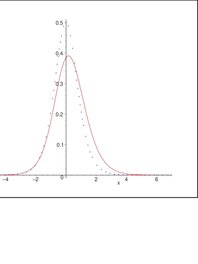
Figure 1: The asymptotic distribution function of $\rho D-\frac{1}{2}\log(L\rho)$ (solid line) and that predicted by the NMW heuristic (dotted line)

As in the NMW model, we could instead have taken the number of shortcuts to be fixed at ${\textstyle{\frac{1}{2}}}L\rho$. Using a standard deviation argument, such a process could with high probability be bracketed by two processes with Poisson numbers of shortcuts, but with different shortcut rates

$$\rho_{1}=\rho\{1-\kappa L^{-1}\sqrt{L\rho}\log(L\rho)\}\quad\mbox{and}\quad\rho_{2}=\rho\{1+\kappa L^{-1}\sqrt{L\rho}\log(L\rho)\},$$

for $\kappa$ big enough. Expanding $\log(L\rho_{1})$ and $\log(L\rho_{2})$ around $\log(L\rho)$, we see that the distributional approximation for the shortest path length would remain the same, for a slightly different region and with different error bounds.

4 $r$ dimensions

Our method of proof can be adapted to many other models. Here, we consider only the generalization of the previous continuous circle model to higher dimensions, taking ${\rm Po\,}(L\rho/2)$ shortcuts between random pairs of points in a finite, homogeneous space $C$ in $r$ dimensions, such as a sphere or a torus, where $L$ is the area of $C$. We construct the shortcuts by a “growth and merge” process as before, but now with intervals replaced by local neighbourhoods of the form $\zeta+tK$ after growth time $t$, where $\zeta$ is the centre and $K\ni 0$ is a given convex set in $r$ dimensions. The basic Poisson approximation of Theorem 3.1 can be applied as before; we then need to find an appropriate $\tau_{x}$, and to make the necessary computations for the associated pure growth process. In particular, we shall need to be able to approximate the sums

$$\sum_{i=1}^{m}\sum_{j=1}^{n}p(s_{i},u_{j}),$$ (4.1)

where $p(s_{i},u_{j})$ is the probability that two independently and randomly distributed sets, one an $s_{i}K$ and the other a $u_{j}K$, intersect one another. We assume this probability to be of the form

$$p(s_{i},u_{j})=L^{-1}\sum_{l=0}^{r}\alpha_{l}s_{i}^{l}u_{j}^{r-l}\quad\mbox{ for constants\ }\alpha_{l}=\alpha_{r-l}.$$ (4.2)

In one dimension, as in the previous section, $\alpha_{0}=\alpha_{1}=2$; for a torus in two dimensions with $K$ a unit square $[-1,1]^{2}$, $\alpha_{0}=\alpha_{1}/2=\alpha_{2}=4$. For a sphere in two dimensions, it is almost the case, neglecting curvature, that $\alpha_{0}=\alpha_{1}/2=\alpha_{2}=\pi$, and the error in using this approximation is negligible for large $L$, to our order of approximation. As in 1–dimension, we shall also have to discount intersections of neighbourhoods where one is entirely contained in the other.

For the pure growth process with independently and uniformly positioned neighbourhoods, define its neighbourhood size process by the purely atomic measure $(\xi_{t},\,t\geq 0)$ on ${\bf R}_{+}$:

$$\xi_{t}(A)=\#\{\mbox{neighbourhoods with radii having lengths in\ }A\}.$$

Then the quantities

$$M_{l}(t):=\int_{{\bf R}_{+}}x^{l}\xi_{t}(dx),\quad l\geq 0,$$

are basic to our analysis: $M_{0}(t)$ is just the number of neighbourhoods in the pure growth process at time $t$, corresponding to $M(t)$ in the circle model, and

$$M_{l}(t)=\sum_{j=1}^{M_{0}(t)}s_{j}^{l}$$

is the sum of the $l$’th powers of the ‘radii’ of the neighbourhoods. In particular, in view of (4.1) and (4.2), the analogue of $\lambda_{(m,n,{\bf s},{\bf u})}$ of Corollary 3.2 is easily expressible for two pure growth processes ${\bf M}$ and ${\bf N}$ at time $t$ as

$$L^{-1}\left\{\sum_{l=0}^{r}\alpha_{l}M_{l}(t)N_{r-l}(t)-v(K)\int_{0}^{t}(N_{r}(u)dM_{0}(u)+M_{r}(u)dN_{0}(u))\right\},$$ (4.3)

where $v(K)$ is the volume of $K$.

The quantities $M_{l}(t)$, $0\leq l\leq r$, satisfy the following evolution equations:

$$\frac{d}{dt}M_{i}(t)=iM_{i-1}(t),\quad i\geq 2;$$

$$\frac{d}{dt}M_{1}(t)=M_{0}(t)\quad\mbox{for a.e. }t;$$ (4.4)

$$M_{0}(t)-\rho rv(K)\int_{0}^{t}M_{r-1}(u)du=X_{0}(t),$$

where $X_{0}$ is a martingale, with $X_{0}(0)=1$ and with (centred) Poisson innovations having rate $\rho rv(K)M_{r-1}(t)$ at time $t$. Properties of their solution are given in the following theorem.

Theorem 4.1

Let ${\bf M}(t)$ denote the $(r+1)$-vector $(M_{0}(t),\ldots,M_{r}(t))^{T}$. Then, as $t\to\infty$,

$${\bf E}{\bf M}(t)\sim r^{-1}e^{\lambda_{0}t}{\bf e}^{(0)};\quad{\bf E}M_{0}^{2}(t)=O(e^{2\lambda_{0}t}),$$

where

$$\lambda_{0}=\lambda_{0}(\rho):=(r!\rho v(K))^{\frac{1}{r}};\ \ {\bf e}^{(0)}=(1,\lambda_{0}^{-1},2\lambda_{0}^{-2},\ldots,(r-1)!\lambda_{0}^{-(r-1)},r!\lambda_{0}^{-r})^{T}.$$

Furthermore,

$${\bf W}(t) := {\bf M}(t)e^{-\lambda_{0}t}\rightarrow{\bf e}^{(0)}W\mbox{ a.s.},$$

where

$$W:=\frac{1}{r}\left\{1+\int_{0}^{\infty}e^{-\lambda_{0}y}dX_{0}(y)\right\}$$

satisfies ${\bf P}[W>0]=1$, and

$$(j!)^{-1}\lambda_{0}^{j}{\bf E}|W_{j}(t)-W{\bf e}^{(0)}_{j}|\leq c_{r}\left(1+(\lambda_{0}t)^{1/2}1_{\{r=6\}}\right)e^{-\lambda_{0}(1-\omega_{*})t},\quad 0\leq j\leq r,$$

for some constant $c_{r}$ not depending on $\rho$, where

$$\omega_{*}=\max\{0,\cos(2\pi/r)\}.$$

Remark.  The fact that $W_{0}(t)\to W$ a.s. implies that

$$M_{0}(t)^{-1}\xi_{t}\{[0,b)\}=1-W_{0}(t-b)e^{-\lambda_{0}b}/W_{0}(t)\to 1-e^{-\lambda_{0}b}$$

for all $b>0$, so that the form of ${\bf e}^{(0)}$ is not surprising.

Proof: Solving (4.4) for the vector ${\bf M}(t)$, we find that

$${\bf M}(t)=Ae^{At}\int_{0}^{t}e^{-Ay}X_{0}(y){\bf\varepsilon^{0}}dy+X_{0}(t){\bf\varepsilon^{0}},$$ (4.5)

where ${\bf\varepsilon^{0}}$ is the coordinate vector $(1,0,0,\ldots,0)^{T}$, and

$$A:=\left(\begin{array}[]{ccccccc}0&&&&0&c&0\\ 1&0&&&&&\\ 0&2&\cdot&&&&\\ \cdot&&&\cdot&&&\cdot\\ \cdot&&&&\cdot&&\cdot\\ \cdot&&&&&\cdot&\cdot\\ 0&&&&0&r&0\end{array}\right)$$

has eigenvalues $\lambda_{r}=0$ and $\lambda_{0},\ldots,\lambda_{r-1}$ satisfying the equation $\lambda^{r}=(r-1)!c$: here, $c=\rho rv(K)$. Thus $\lambda_{0}=\{c(r-1)!\}^{\frac{1}{r}}$ is real and positive, and $\lambda_{l}=\lambda_{0}\omega_{l}$, where $\omega_{l}=e^{2\pi il/r}$ are the complex $r$’th roots of unity.

The eigenvectors ${\bf e}^{(l)}$ of $A$ are also easy to determine. The $r$’th eigenvector ${\bf e}^{(r)}$ is the coordinate vector ${\bf\varepsilon^{r}}=(0,\ldots,0,1)^{T}$, and all others have components $e_{0},\ldots,e_{r}$ satisfying the equations

$$ce_{r-1} = \lambda e_{0};\quad e_{0}=\lambda e_{1};\quad 2e_{1}=\lambda e_{2};\quad\ldots;$$

$$(r-1)e_{r-2} = \lambda e_{r-1};\quad re_{r-1}=\lambda e_{r},$$

for $\lambda=\lambda_{0},\ldots,\lambda_{r-1}$. These in turn give

$$e_{1} = \lambda^{-1}e_{0};\quad e_{2}=2\lambda^{-2}e_{0};\quad\ldots;$$

$$e_{r-1} = (r-1)!\lambda^{-(r-1)}e_{0}=\lambda c^{-1}e_{0};\quad e_{r}=r!\lambda^{-r}e_{0}.$$

Thus it follows that, for $0\leq l\leq r-1$,

$${\bf e}^{(l)}=\left(1,(\lambda_{0}\omega_{l})^{-1},2(\lambda_{0}\omega_{l})^{-2},\ldots,(r-1)!(\lambda_{0}\omega_{l})^{-(r-1)},c^{-1}r\right)^{T}.$$ (4.7)

The eigendecomposition can now be used to determine ${\bf M}(t)$ more explicitly. Writing ${\bf\varepsilon^{0}}$ in terms of the ${\bf e}^{(l)}$, $0\leq l\leq r$, we find that

$${\bf\varepsilon^{0}}=\sum_{l=0}^{r}\mu_{l}{\bf e}^{(l)}\ \ \mbox{with }\ \mu_{0}=\cdots=\mu_{r-1}=r^{-1}\ \mbox{and }\mu_{r}=-r/c.$$

Using this to evaluate (4.5), we obtain

$${\bf M}(t) = \int_{0}^{t}\{(X_{0}(y)-1)+1\}\sum_{l=0}^{r-1}{\bf e}^{(l)}\mu_{l}\lambda_{l}e^{\lambda_{l}(t-y)}dy+X_{0}(t){\bf\varepsilon^{0}}.$$ (4.8)

Turning to the moments of ${\bf M}$, we immediately have

$${\bf E}{\bf M}(t) = \int_{0}^{t}\sum_{l=0}^{r-1}{\bf e}^{(l)}\mu_{l}\lambda_{l}e^{\lambda_{l}(t-y)}dy+{\bf\varepsilon^{0}}$$

$$= \sum_{l=0}^{r-1}\frac{1}{r}\left(e^{\lambda_{0}t\omega_{l}}-1\right){\bf e}^{(l)}+{\bf\varepsilon^{0}}\sim\frac{1}{r}e^{\lambda_{0}t}{\bf e}^{(0)}.$$

To estimate second moments, observe that, given ${\cal F}_{t}$, $dX_{0}(t)$ is a centred Poisson innovation, so that

$${\bf E}\left(d^{2}X_{0}(t)\right)=c{\bf E}(M_{r-1}(t))dt\sim cr^{-1}e^{\lambda_{0}t}{\bf e}^{(0)}_{r-1}\,dt=r^{-1}\lambda_{0}e^{\lambda_{0}t}\,dt.$$ (4.9)

But now, in (4.8), we can write

$$M^{(1,l)}(t):=\int_{0}^{t}(X_{0}(y)-1)\lambda_{l}e^{\lambda_{l}(t-y)}\,dy=\int_{0}^{t}\{e^{\lambda_{l}(t-v)}-1\}\,dX_{0}(v),$$

since $X_{0}$ is a.s. of bounded variation on finite intervals. Hence, from (4.9),

$${\bf E}|M^{(1,l)}(t)|^{2}\leq 2r^{-1}\lambda_{0}\int_{0}^{t}e^{\lambda_{0}v}\{1+e^{2\Re\lambda_{l}(t-v)}\}\,dv.$$ (4.10)

For $1\leq l\leq r-1$, we can bound the integral in (4.10), uniformly in $l$ and $\rho$, in terms of $\omega_{*}$ and $\lambda_{0}(\rho)t$. If $1\leq r\leq 4$, so that $\omega_{*}=0$, it is immediate that ${\bf E}|M^{(1,l)}(t)|^{2}\leq 4r^{-1}e^{\lambda_{0}t}$. If $r=5$, so that $0<\omega_{*}<1/2$, the bound has an extra factor of $1/(1-2\omega_{*})$; if $r=6$, then $\omega_{*}=1/2$, and ${\bf E}|M^{(1,l)}(t)|^{2}\leq 4r^{-1}\lambda_{0}te^{\lambda_{0}t}$; for $r\geq 7$, ${\bf E}|M^{(1,l)}(t)|^{2}\leq 4r^{-1}(2\omega_{*}-1)^{-1}e^{2\lambda_{0}\omega_{*}t}$. In all cases, for all $1\leq l\leq r-1$, we have ${\bf E}|M^{(1,l)}(t)|^{2}=o(e^{2\lambda_{0}t})$, and since also

$${\bf E}|M^{(1,0)}(t)|^{2}\leq r^{-1}\lambda_{0}\int_{0}^{t}e^{2\lambda_{0}t-\lambda_{0}v}\,dv\leq r^{-1}e^{2\lambda_{0}t},$$

it therefore follows easily that

$${\bf E}M_{0}^{2}(t)=O(e^{2\lambda_{0}t})\quad\mbox{as }t\to\infty,$$ (4.11)

with the constant implied in the order estimate uniform for all $\rho$.

The convergence of ${\bf W}(t)$ can now be proved by second moment arguments. It follows directly from (4.9) that ${\rm Var\,}X_{0}(t)=r^{-1}(e^{\lambda_{0}t}-1)$, and thus, using Kolmogorov’s inequality on the martingale $X_{0}$, we can easily show that, for any $\delta>0$,

$$\sup_{t>0}|X_{0}(t)-1|e^{-(\lambda_{0}+\delta)t/2}<\infty.$$ (4.12)

Now, from (4.8),

$${\bf W}(t) = e^{-\lambda_{0}t}{\bf M}(t)$$ (4.13)

$$= e^{-\lambda_{0}t}{\bf E}{\bf M}(t)+e^{-\lambda_{0}t}(X_{0}(t)-1){\bf\varepsilon^{0}}$$

$$+\int_{0}^{t}(X_{0}(y)-1)\sum_{l=0}^{r-1}{\bf e}^{(l)}\mu_{l}\lambda_{l}e^{\lambda_{l}(t-y)}dye^{-\lambda_{0}t},$$

and we consider the various terms in (4.13), using (4.12). First, it is immediate that

$$\lim_{t\to\infty}e^{-\lambda_{0}t}(X_{0}(t)-1)=0\mbox{ a.s.}$$

Then, distinguishing the cases $\Re(\lambda_{l})\leq 0$, $0<\Re(\lambda_{l})\leq\lambda_{0}/2$ and $\lambda_{0}/2<\Re(\lambda_{l})<\lambda_{0}$, it again follows from (4.12) that, for $1\leq l\leq r-1$,

$$\lim_{t\to\infty}\int_{0}^{t}(X_{0}(y)-1)\mu_{l}\lambda_{l}e^{\lambda_{l}(t-y)-\lambda_{0}t}\,dy=0\mbox{ a.s.}$$

Finally, for $l=0$, we have

$$\lim_{t\to\infty}\int_{t}^{\infty}(X_{0}(y)-1)\lambda_{0}e^{-\lambda_{0}y}\,dy=0\mbox{ a.s.}$$

Hence, letting $t\to\infty$ in (4.13), it follows that the limit

$$\lim_{t\to\infty}{\bf W}(t) = {\bf e}^{(0)}\frac{1}{r}\left\{1+\int_{0}^{\infty}\lambda_{0}(X_{0}(y)-1)e^{-\lambda_{0}y}dy\right\}=W{\bf e}^{(0)}$$

exists a.s. To show that ${\bf P}[W>0]=1$, note that

$$W=\sum_{l\geq 1}e^{-\lambda_{0}U_{l}}W^{(l)},$$

where $(U_{l},\,l\geq 1)$ are the times of the births of new neighbourhoods as children of the original neighbourhood around $P$, and $(W^{(l)},\,l\geq 1)$ are independent copies of $W$. This immediately implies that ${\bf P}[W=0]\in\{0,1\}$, and ${\bf P}[W=0]=1$ is excluded by ${\bf E}W=1/r$.

Note also that, again because $X_{0}$ is locally of bounded variation,

$${\bf W}(\infty)-{\bf W}(t)$$

$$= \mu_{0}{\bf e}^{(0)}e^{-\lambda_{0}t}-\sum_{l=1}^{r-1}{\bf e}^{(l)}\mu_{l}e^{-\lambda_{0}t}\left(e^{\lambda_{l}t}-1\right)$$

$$-{\bf\varepsilon^{0}}e^{-\lambda_{0}t}+\mu_{0}{\bf e}^{(0)}\int_{t}^{\infty}e^{-\lambda_{0}y}dX_{0}(y)$$

$$\qquad-\sum_{l=1}^{r-1}{\bf e}^{(l)}\mu_{l}\lambda_{l}e^{-(\lambda_{0}-\lambda_{l})t}\int_{0}^{t}\frac{e^{-\lambda_{l}y}-e^{-\lambda_{l}t}}{\lambda_{l}}dX_{0}(y)$$

$$= \mu_{0}{\bf e}^{(0)}e^{-\lambda_{0}t}-\sum_{l=1}^{r-1}{\bf e}^{(l)}\mu_{l}e^{-\lambda_{0}t}\left(e^{\lambda_{l}t}-1\right)$$

$$-{\bf\varepsilon^{0}}e^{-\lambda_{0}t}+\mu_{0}{\bf e}^{(0)}\int_{t}^{\infty}e^{-\lambda_{0}y}dX_{0}(y)$$

$$\qquad-\sum_{l=1}^{r-1}{\bf e}^{(l)}\mu_{l}\int_{0}^{t}dX_{0}(y)\left\{e^{-\lambda_{0}t+\lambda_{l}(t-y)}-e^{-\lambda_{0}t}\right\}.$$

Thus

$$(j!)^{-1}\lambda_{0}^{j}|{\bf E}(W_{j}(\infty)-W_{j}(t))|\leq c_{r1}e^{-\lambda_{0}(1-\omega_{*})t}$$ (4.14)

and, from (4.9),

$${\rm Var\,}\{(j!)^{-1}\lambda_{0}^{j}(W_{j}(\infty)-W_{j}(t))\}\leq c_{r2}e^{-2\lambda_{0}(1-\omega_{*})t}\{1+(\lambda_{0}t)1_{\{r=6\}}\},$$ (4.15)

for some constants $c_{r1}$ and $c_{r2}$ and for all $0\leq j\leq r$, completing the proof. $[]$

Now choose

$$\tau_{x}:={1\over\lambda_{0}(\rho)}\left\{\frac{1}{2}\log(L\rho)+x\right\},$$ (4.16)

for any $x$ such that $|x|\leq\frac{1}{4}\log(L\rho)$, much as in the case $r=1$. Let ${\widehat{V}}_{x}$ as before be the number of pairs of overlapping neighbourhoods, one from each of two independent pure growth processes ${\bf M}(\tau_{x})$ and ${\bf N}(\tau_{x})$ and neither contained entirely in the other. Then, from (4.3) and Theorem 3.1, it follows easily that $\displaystyle\left|{\bf P}[{\widehat{V}}_{x}=0]-{\bf E}\exp\left\{-L^{-1}\left(\sum_{l=0}^{r}\alpha_{l}M_{l}(\tau_{x})N_{r-l}(\tau_{x})\right.\right.\right.$ $\displaystyle\qquad\qquad\qquad\left.\left.\left.\mbox{}-v(K)\int_{0}^{\tau_{x}}(N_{r}(u)dM_{0}(u)+M_{r}(u)dN_{0}(u))\right)\right\}\right|$ $\displaystyle\qquad=O((L\rho)^{-1/2}\log^{r}(L\rho)e^{x}),$ (4.17) since the probability of a given pair of neighbourhoods overlapping cannot exceed

$$L^{-1}\kappa v(K)\tau_{x}^{r}=O((L\rho)^{-1}\log^{r}(L\rho)),$$

for some constant $\kappa$ depending on the shape of $K$, and because ${\bf E}M_{0}(\tau_{x})\sim r^{-1}(L\rho)^{1/2}e^{x}$ from Theorem 4.1. Then, with a proof much as for Lemma 3.4, bounding $M_{0}$ above by a Yule process with rate $\rho v(K)r\tau_{x}^{r-1}$ and noting that we now only have ${\bf P}[A^{l}(i)=l]\leq 1/l$, because in higher dimensions more recent neighbourhoods grow more slowly, it follows that

$${\bf P}[{\widehat{V}}_{x}\neq V_{x}]=O((L\rho)^{-1/2}\log^{2r}(L\rho)e^{3x}),$$ (4.18)

where $V_{x}$ is the number of times that pairs of neighbourhoods of the two associated growth and merge processes $R$ and $R^{\prime}$ meet before $\tau_{x}$. These observations lead to the following theorem.

Theorem 4.2

Let $D$ denote the distance between two randomly chosen points of $C$ on the graph with a ${\rm Po\,}(L\rho/2)$–distributed random number of shortcuts. Then

$${\bf P}\left[D>{2\over\lambda_{0}(\rho)}\left\{\frac{1}{2}\log(L\rho)+x\right\}\right]$$

$$\qquad={\bf E}\left(\exp\left\{-e^{2x}WW^{\prime}\left[{1\over v(K)}\sum_{l=0}^{r}{\alpha_{l}\over{r\choose l}}-1\right]\right\}\right)$$

$$\qquad\qquad+O\left\{(L\rho)^{-(1-\omega_{*})/2}\log^{2r+1}(L\rho)(e^{3x}+e^{x})\right\},$$

uniformly in $|x|\leq\frac{1}{4}\log(L\rho)$, where $W$ and $W^{\prime}$ are independent copies of the limiting random variable of Theorem 4.1.

Proof: In view of (4.17) and (4.18), it is enough to show that

$${\bf E}\exp\left\{-L^{-1}\left(\sum_{l=0}^{r}\alpha_{l}M_{l}(\tau_{x})N_{r-l}(\tau_{x})-v(K)\int_{0}^{\tau_{x}}(N_{r}(u)dM_{0}(u)+M_{r}(u)dN_{0}(u))\right)\right\}$$

$$={\bf E}\left(\exp\left\{-e^{2x}WW^{\prime}\left[{1\over v(K)}\sum_{l=0}^{r}{\alpha_{l}\over{r\choose l}}-1\right]\right\}\right)+O(\lambda_{0}\tau_{x}\exp\{2x-\lambda_{0}(1-\omega_{*})\tau_{x}\}).$$

However, direct calculation shows that

$$L^{-1}\sum_{l=0}^{r}\alpha_{l}M_{l}(\tau_{x})N_{r-l}(\tau_{x})={e^{2x}\over r!v(K)}\sum_{l=0}^{r}\alpha_{l}\{\lambda_{0}^{l}W_{l}(\tau_{x})\}\,\{\lambda_{0}^{r-l}W^{\prime}_{r-l}(\tau_{x})\}$$

and that

$$L^{-1}v(K)\int_{0}^{\tau_{x}}(N_{r}(u)dM_{0}(u)+M_{r}(u)dN_{0}(u))$$

$$= L^{-1}v(K)\left\{\vphantom{\int_{0}^{\tau_{x}}}e^{2\lambda_{0}\tau_{x}}\{W_{0}(\tau_{x})W_{r}^{\prime}(\tau_{x})+W_{0}^{\prime}(\tau_{x})W_{r}(\tau_{x})\right.$$

$$\qquad\left.\mbox{}-r\int_{0}^{\tau_{x}}e^{2\lambda_{0}u}\{W_{0}(u)W^{\prime}_{r-1}(u)+W_{0}^{\prime}(u)W_{r-1}(u)\}\,du\right\}$$

$$= e^{2x}\left(W_{0}(\tau_{x})\{\rho v(K)W_{r}^{\prime}(\tau_{x})\}\vphantom{I_{1}^{1}}+W^{\prime}_{0}(\tau_{x})\{\rho v(K)W_{r}(\tau_{x})\}\right)$$

$$\qquad\mbox{}-\frac{1}{L\rho}\int_{0}^{\tau_{x}}\lambda_{0}e^{2\lambda_{0}u}\left(W_{0}(u)\{\lambda_{0}^{-1}r\rho v(K)W^{\prime}_{r-1}(u)\}\right.$$

$$\qquad\qquad\qquad\qquad\qquad\qquad\left.\mbox{}+W^{\prime}_{0}(u)\{\lambda_{0}^{-1}r\rho v(K)W_{r-1}(u)\}\right)\,du$$

where, by Theorem 4.1,

$${\bf E}|(j!)^{-1}\lambda_{0}^{j}W_{j}(t)-W|\leq c_{r}(1+(\lambda_{0}t)^{1/2}1_{\{r=6\}})e^{-\lambda_{0}(1-\omega_{*})t},\quad 0\leq j\leq r,$$

in which, for $j=0,r-1$ and $r$, the left hand side takes the form ${\bf E}|W_{0}(t)-W|$, ${\bf E}|\lambda_{0}^{-1}r\rho v(K)W_{r-1}(t)-W|$ and ${\bf E}|\rho v(K)W_{r}(t)-W|$ respectively. Then the inequality $|e^{-a}-e^{-b}|\leq|a-b|$ for all $a,b\geq 0$ completes the proof. $[]$

Note that in the $r$–dimensional model, the distances $D$ have $\lambda_{0}(\rho)$ in the denominator, of order $O(\rho^{1/r})$, in place of $2\rho$ in the case $r=1$. This scaling can be understood as follows. If there were no shortcuts, the average distance between pairs of points would be of order $L^{1/r}$. With about $L\rho/2$ shortcuts, this distance is reduced by a factor of order $(L\rho)^{-1/r}\log(L\rho)$. Thus, in a higher dimensional space, the reduction in distance as a result of introducing shortcuts is correspondingly smaller.

Acknowledgement. The authors would like to thank A.G. Pakes for sharing his expertise on the limiting variable $W$. Moreover the authors are grateful to the referees for an extremely careful reading of the paper, and for many valuable comments.

References

• [1] Ball, F., Mollison, D. and Scalia-Tomba, G. (1997). Epidemics with two levels of mixing. Ann. Appl. Probab. 7, 46–89.
• [2] Barbour, A.D., Holst, L. and Janson, S. (1992). Poisson Approximation. Oxford Science Publications.
• [3] Barrat and Weigt (2000). On the properties of small-world network models. Europhysics Journal B 13, 547–560.
• [4] Bollobas, B. (1985). Random Graphs. Academic Press, London.
• [5] Moore, C. and Newman, M.E.J. (1999). Epidemics and percolation in small-world networks. Santa Fe Institute working paper 00-01-002. Also http://xxx.lanl.gov/archive/cond-mat/9911492.
• [6] Newman, M.E.J. and Watts, D.J. (1999). Scaling and percolation in the small-world network model. Phys. Rev. E 60, 7332–7344.
• [7] Newman, M.E.J., Moore, C. and Watts, D.J. (1999). Mean-field solution of the small-world network model. Santa Fe Institute working paper 99-09-066. Also
http://xxx.lanl.gov/archive/cond-mat/9909165.
• [8] Ross, S.M. (1996). Stochastic Processes, 2nd edition. Wiley, New York.
• [9] Watts, D.J. (1999). Small Worlds. Princeton University Press.
• [10] Watts, D.J. and Strogatz, S.H. (1998). Collective dynamics of “small-world” networks. Nature 393, 440–442.