A dual point description of mesoscopic superconductors

Abstract

We present an analysis of the magnetic response of a mesoscopic superconductor, i.e. a system of sizes comparable to the coherence length and to the London penetration depth. Our approach is based on special properties of the two dimensional Ginzburg-Landau equations, satisfied at the dual point $(\kappa=\frac{1}{\sqrt{2}}).$ Closed expressions for the free energy and the magnetization of the superconductor are derived. A perturbative analysis in the vicinity of the dual point allows us to take into account vortex interactions, using a new scaling result for the free energy. In order to characterize the vortex/current interactions, we study vortex configurations that are out of thermodynamical equilibrium. Our predictions agree with the results of recent experiments performed on mesoscopic aluminium disks.

PACS: 74.25.Ha, 74.60.Ec, 74.80.-g

I Introduction

The ability to detect and manipulate vortices with great sensivity in systems of small size such as mesoscopic superconductors [1] or atomic condensates [2] has generated an outgrow of interest in the mechanism of creation and annihilation of vortices and in the study of stable and metastable vortex configurations. In particular, recent advances in the technique of Hall magnetometry [3] have allowed to measure the magnetization of small superconducting samples containing only a few vortices [1, 4]. These experiments are conducted on aluminium disks well below the superconducting transition temperature, whereas previous measurements were performed only in the vicinity of the normal/superconductor phase boundary [5, 6]. Besides, the magnetization measurements in [1] are carried out on an individual disk and not on an ensemble of disks as in [6]. The radius $R$ and the thickness $d$ of the sample used in the experiments are comparable to the superconducting characteristic lengths, i.e. the London penetration length ($\lambda=$ 70nm) and the coherence length ($\xi=$250nm). Such a sample can neither be considered to be macroscopic, nor microscopic. The system falls, rather, in a mesoscopic regime where surface effects are of the same order of magnitude as the bulk effects. Thus, the magnetic response of a mesoscopic superconducting disk to an applied field depends strongly on its size and is very different from that of a macroscopic superconductor. When the radius $R$ of the sample is much smaller than the coherence length $\xi$, no vortex can nucleate, the normal/superconductor phase transition is second order and the magnetization $M$, as a function of the external applied field $H_{e}$, has a non-linear behaviour (non-linear Meissner effect [7, 8]). If $R$ is comparable to $\xi$, the superconducting phase transition is first order and a bistable hysteresis region appears in the $M-H_{e}$ curve. For $R$ greater than $\xi$, the phase transition is again second order, and when the applied field exceeds a critical value $H_{1}$, the magnetization curve exhibits a series of discontinuous jumps corresponding to the successive entry of vortices into the sample. This qualitative interpretation is supported, at least for low applied magnetic fields, by the periodicity of the jumps which corresponds to the entrance of an additional superconducting quantum of flux into the disk. For larger fields, or equivalently for higher density of vortices, both the period and the height of the jumps become smaller, a behaviour related to the interactions between the vortices and to transitions between stable vortex configurations, with the same number of vortices.

The magnetization shows also a hysteretic behaviour depending on the direction of the field sweep, due to the presence of a confining energy barrier (the absence of remanent magnetization precludes pinning effects). In some metastable states, the sample may exhibit even a paramagnetic response [4] whereas in thermodynamic equilibrium a superconductor is diamagnetic.

These experimental results have led to a renewed interest in the theory of mesoscopic superconductors. Numerical computations have shown that the phenomenological Ginzburg-Landau theory is well suited to describe a superconducting sample in the mesoscopic regime, even far from the critical temperature. These works have revealed physical phenomena that play an important role in such systems (for a review see [7]), like: the role of surface barriers for vortex nucleation and hysteresis [9, 10, 11]; the interplay between vortex/vortex and vortex/edge interactions that explains vortex structures in mesoscopic disks [10, 9]; the transition between a giant multiple vortex state and a state with several vortices carrying a unit quantum of flux [12].

The Ginzburg-Landau free energy of a superconductor involves two fields, the (complex) order parameter $\psi=|\psi|e^{i\chi}$ and the vector potential ${\vec{A}}$. The minimization of this free energy leads to a set of two coupled non-linear partial differential equations for $\psi$ and ${\vec{A}}$, involving the two characteristic lengths $\lambda$ and $\xi.$ But the solutions depend only on one relevant number, the phenomenological Ginzburg-Landau parameter $\kappa$ defined by

$$\kappa=\frac{\lambda}{\xi}\;.$$ (1)

A macroscopic superconductor is said to be of type I if $\kappa<\frac{1}{\sqrt{2}}$ and of type II if $\kappa>\frac{1}{\sqrt{2}}.$ A macroscopic superconductor of Type II admits a stable Abrikosov vortex lattice phase when the applied field $H_{e}$ lies between the first penetration field and the upper critical field [13]. For aluminium, $\kappa$ is smaller than $\frac{1}{\sqrt{2}}$, hence a macroscopic sample of Al is a type I superconductor.

Analytical studies of the Ginzburg-Landau equations in two-dimensional systems require the use of various approximations since, in general, exact solutions can not be found due to the non-linearity. One approach is to linearize the equations assuming $|\psi|\ll 1,$ and to decouple them by supposing that the magnetic field $B$ in the sample is equal to the applied field $H_{e}$. This approach describes correctly the superconducting/normal phase boundary [5, 6, 14, 15, 16], but fails to explain the behaviour of the sample deep inside the superconducting state. For example, in the linearized theory, all the vortices are at the center of the disk [16] and therefore one can not study the role of surface barriers, the interaction between vortices, and the fragmentation of a giant vortex into unit vortices. Besides, the critical fields corresponding to the successive entrance of vortices into the sample do not scale correctly with the size of the system (e.g. experimentally, the entrance field $H_{1}$ of the first vortex scales as ${R}^{-1}$ whereas the linear theory predicts a ${R}^{-2}$ dependence). Of course, in the vicinity of the upper critical field [16] the linearized theory agrees quantitatively with the experimental results.

A second approach is to use the London equation which can be derived from the Ginzburg-Landau equations by supposing that $|\psi|=1$ everywhere except on a finite number of isolated points, called vortices, where $|\psi|=0.$ London’s equation is valid rigorously when the parameter $\kappa$ goes to infinity, i.e. for extreme type II superconductors in which vortices are indeed point-like. Many theoretical results have been derived from the London equation, such as discrete nucleation of flux lines in a thin cylinder [17, 18] or in a thin disk [19, 20], the existence of surface energy barriers [13, 21], and the computation of polygonal ring configurations of vortices in finite samples [22, 23]. However, when $\kappa\to\infty,$ the minimum energy is obtained for one flux quantum per vortex [24, 25] and vortices have a hard-core repulsive interaction impeding the formation of a giant vortex state. Moreover, the surface energy barriers calculated from London’s equation are quantitatively different from those obtained by numerically solving the Ginzburg-Landau equations [26]. In fact, the experimental conditions are far off the London limit, although thin Al disks are likely to have an effective $\kappa$ greater than its measured value [1] of 0.28 (in a thin disk, one can argue, following [19], that the effective London length is of the order of ${\lambda^{2}}/{d}$, and this results in a higher value of $\kappa$).

We follow another approach, less explored in the literature, based on an exact result for the two-dimensional Ginzburg-Landau equations. In an infinite plane reduce to first order differential equations that can be decoupled when the parameter $\kappa$ takes the special value $1/{\sqrt{2}},$ called the dual point[24, 25, 27]. At that point, the free energy is a topological invariant of the system. In [28], we generalized this method to a finite domain with boundaries; this enabled us to classify solutions with different number of vortices and to derive analytical expressions for the free energy and the magnetization of a mesoscopic disk as a function of the applied field. Our results agreed qualitatively with the experimental data, and even quantitatively when the number of vortices in the system is low. However, some important features such as the non-linear Meissner effect in a fractional fluxoid disk, the variation of the amplitude and the period of the jumps in the $M-H_{e}$ curve could not be described. Moreover, in [28], we discussed only the case where $R$ is much larger than $\xi$ and did not obtain the different regimes of the magnetization curve when the ratio $R/\xi$ is varied.

In this paper, we study the Ginzburg-Landau free energy ${\cal F}$ not only at the dual point $\kappa=1/{\sqrt{2}}$ but also in its vicinity where vortices start to interact weakly [29]. Taking into account non-linear effects, our calculations describe the magnetic response of the sample as its size changes, providing an understanding of the non-linear Meissner effect and of the multi-vortex state. We shall also study non-equilibrium vortex configuration in order to determine the interaction between a vortex and edge currents.

The plan of this paper goes as follows: in section 2, some basic features of the Ginzburg-Landau theory of superconductivity are recalled. In section 3, after studying the case of an infinite system, we generalize the Bogomol’nyi’s approach to a finite size superconductor and calculate its free energy at the dual point. This result is applied to an infinite cylinder in section 4. The case of a mesoscopic disk is studied in section 5 and magnetization curves are obtained for systems of different sizes. In section 6, we obtain the free energy and the magnetization of a cylindrically symmetric system when $\kappa$ is close to the dual point. The surface energy barrier for a one vortex state out of thermodynamic equilibrium is calculated in section 7. In the last section we discuss our results and suggest some further generalizations. Some mathematical details are included in the two appendices.

II The Ginzburg-Landau theory of superconductivity

We recall here some basic features of the Ginzburg-Landau theory and define our notations. The order parameter $\psi=|\psi|e^{i\chi}$ is a complex number and the potential vector ${\vec{A}}$ satisfies ${\vec{\nabla}}\times{\vec{A}}={\vec{B}}$, where ${\vec{B}}$ is the local magnetic induction. The two characteristic lengths $\lambda$ and $\xi$ appear as phenomenological parameters. In this work, we measure lengths in units of $\lambda{\sqrt{2}}$, the magnetic field in units of $\frac{\phi_{0}}{4\pi\lambda^{2}}$ and the vector potential in units of $\frac{\phi_{0}}{2\sqrt{2}\pi\lambda}$ where the flux quantum $\phi_{0}$ is given by $\phi_{0}=\frac{hc}{2e}.$ The Ginzburg-Landau free energy $\cal F$, defined as the difference of the free energies ${\cal F}=F_{S}(B)-F_{S}(0)$, is measured in units of $\frac{H_{c}^{2}}{4\pi}$ where ${H_{c}}$ the thermodynamic field satisfies ${H_{c}}={\sqrt{2}}\kappa\frac{\phi_{0}}{4\pi\lambda^{2}}$. In these units, $\cal F$ is given by

$${\cal F}={\int_{\Omega}}{1\over 2}|B{|^{2}}+{\kappa^{2}}|1-|\psi{|^{2}}{|^{2}}+|({\vec{\nabla}}-i{\vec{A}})\psi{|^{2}}\,\,\,\,\,\,,$$ (2)

where the integration is over the superconducting domain $\Omega$. The Ginzburg-Landau equations that minimize ${\cal F}$, become

$$-({\vec{\nabla}}-i{\vec{A}})^{2}\psi = 2{\kappa}^{2}\psi(1-|\psi{|^{2}})$$ (3)

$${\vec{\nabla}}\times{\vec{B}} = 2{\vec{\jmath}}$$ (4)

Equation (4) is the Maxwell-Ampère equation with a current density ${\vec{\jmath}}=\mbox{Im}({{\psi^{*}}}{\vec{\nabla}}\psi)-|\psi{|^{2}}{\vec{A}}$ related to the superfluid velocity ${\vec{v}_{s}}$ by

$${\vec{v}_{s}}={{\vec{\jmath}}\over|\psi{|^{2}}}={\vec{\nabla}}\chi-{\vec{A}}$$ (5)

Outside the superconducting sample, $\psi=0.$ The boundary condition on the surface of the superconductor is obtained by requiring that the normal component of the current density vanishes (superconductor/insulator boundary condition [13]):

$$({\vec{\nabla}}-i{\vec{A}})\psi|_{\hat{\bf n}}=0$$ (6)

here ${\hat{\bf n}}$ is the unit vector normal at each point to the surface of the superconductor.

The London fluxoid is the quantity $\left(\displaystyle{{\vec{\jmath}}\over{|\psi|^{2}}}+{\vec{A}}\right),$ that is identical to ${\vec{\nabla}}\chi$. Since $\chi$ is the phase of the univalued function $\psi,$ the circulation of the London fluxoid along a closed contour ${\cal C}$ is quantized [13, 30]:

$$\oint_{\cal C}(\frac{{\vec{\jmath}}}{|\psi{|^{2}}}+{\vec{A}}).{\vec{d}l}=\oint_{\cal C}{\vec{\nabla}}\chi.{\vec{d}l}=2\pi n$$ (7)

The integer $n$ is the winding number of the phase of the system along the contour ${\cal C}$ and is a topological characteristic of the system.

In this study, the superconducting sample is either an infinite cylinder or a thin disk, with cross-section of radius $R$, placed in an external magnetic field parallel to its axis. Since $R$ is an important parameter, we define the dimensionless quantity:

$$a=\frac{\lambda\sqrt{2}}{R}$$ (8)

$a$ is supposed to be small compared to 1 (typically $a\sim 1/10$ in the experiments) unless stated otherwise. The flux created by the external and uniform magnetic field $H_{e}$ (expressed in units of $\frac{\phi_{0}}{4\pi\lambda^{2}}$) through the cross section $\pi R^{2}$ of the sample is equal to $\pi R^{2}H_{e}\frac{\phi_{0}}{4\pi\lambda^{2}}=\frac{H_{e}}{2a^{2}}\phi_{0}.$ The flux $\phi_{e}$, in units of the flux quantum $\phi_{0}$, is thus given by:

$$\phi_{e}=\frac{H_{e}}{2a^{2}}$$ (9)

We emphasize that, in the units we have chosen, the flux $\phi_{b}$ of a magnetic field $\vec{B}$ through a surface $\Omega$ is obtained via the following formula:

$$\phi_{b}=\frac{1}{2\pi}\int_{\Omega}{\vec{B}}.{\vec{d}S}=\frac{1}{2\pi}\oint_{\partial\Omega}{\vec{A}}.{\vec{d}l}$$ (10)

An extra factor $1/{2\pi}$ appears here because $B$ is given in units of $\frac{\phi_{0}}{4\pi\lambda^{2}}$, the surface in units of $2\lambda^{2}$ and the flux in units of $\phi_{0}$.

Since we are studying a superconductor in an applied external field, the relevant thermodynamic potential is the Gibbs free energy $G$ obtained from $F$ via a Legendre transformation:

$$G=F-H_{e}\int_{\Omega}B=F-H_{e}2\pi\phi_{b}=F-4\pi a^{2}\phi_{e}\phi_{b}$$ (11)

In a normal sample, $\psi=0$ and $B=H_{e}$. Therefore, the Gibbs free energy $G_{N}$ of a normal sample is given by:

$$G_{N}=F_{N}-H_{e}\int_{\Omega}B=F_{N}-2\pi a^{2}\phi_{e}^{2}$$ (12)

At thermodynamic equilibrium, the superconductor selects the state of minimal Gibbs free energy. The quantity that we are interested in, and which is measured in experiments, is the magnetization $M$ of the superconductor due to the applied field given by $4\pi M=B-H_{e}$. It is obtained, at thermodynamic equilibrium and up to a constant equal to the superconducting condensation energy, from the difference of the (dimensionless) Gibbs energies

$${\cal G}=G_{S}-G_{N}={\cal F}+2\pi a^{2}\phi_{e}^{2}-4\pi a^{2}\phi_{e}\phi_{b}$$ (13)

using the thermodynamic relation [13]:

$$-M=\frac{1}{2\pi}\frac{\partial{\cal G}}{\partial\phi_{e}}$$ (14)

III Free energy of a superconductor at the dual point

We now study the particular case of the dual point, defined by $\kappa={1\over\sqrt{2}}.$ For this value of the Ginzburg-Landau parameter, the free energy (2) of a two dimensional domain ${\Omega}$ can be written as [25, 28]:

$${\cal F}={\int_{\Omega}}\left({1\over 2}\left(B-1+|\psi|^{2}\right)^{2}+|{\cal D}\psi{|^{2}}\right)+{\oint_{\partial\Omega}}({\vec{\jmath}}+{\vec{A}}).{\vec{d}l}$$ (15)

where the operator $\cal D$ is defined as ${\cal D}=\partial_{x}+i\partial_{y}-i(A_{x}+iA_{y})$ and the second integral is over the boundary of the domain ${\Omega}.$

A The case of an infinite system

If we suppose that the domain ${\Omega}$ is infinite and superconducting at large distances [25], i.e. $|\psi|\to 1$ at infinity, then the boundary integral in (15) is identical to the fluxoid. Using the quantization property (7), we obtain

$${\cal F}=2\pi n+{\int_{\Omega}}\left({1\over 2}(B-1+|\psi|^{2})^{2}+|{\cal D}\psi|^{2}\right)$$ (16)

The free energy is thus minimum when Bogomol’nyi equations [25] are satisfied, that is when,

$${\cal D}\psi = 0$$ (17)

$$B = 1-|\psi|^{2}$$ (18)

Thus, the total free energy results only from the boundary term in (15) and is a purely topological number:

$${\cal F}=2\pi n\,\,\,\,.$$ (19)

The free energy is proportional to the number of vortices: at the dual point, vortices do not interact with each other [25, 29].

B Finite size systems

In a finite system with boundaries, vortices do not interact with each other at the dual point but they are repelled by the edge currents. Therefore, at thermodynamic equilibrium, all vortices collapse into a giant vortex state. Since the superconductor under discussion has a circular cross-section, this giant vortex (or multi-vortex) is located at the center and the system is invariant under cylindrical symmetry. In a finite size mesoscopic superconductor at the dual point, the boundary integral, in (15), can not be identified with the fluxoid because $|\psi|$ is in general different from 1 on the boundary of the system. This quantity is no more a topological integer but a continuously varying real number. The two terms of (15) can not, therefore, be minimized separately to obtain the optimal free energy. In [28], we found a method to circumvent this difficulty: if the system is invariant under cylindrical symmetry, i.e. all the vortices are at the center of the disk, then the current density has only an azimuthal component $\jmath_{\theta}$. The current $\jmath_{\theta}$ has opposite signs near the center (where the vortex is located) and at the edge of the disk (where Meissner currents oppose the penetration of the external field). Hence, there exists a circle $\Gamma$ on which $\jmath_{\theta}$ vanishes [28]. Along $\Gamma$, we have

$${\vec{\jmath}}+{\vec{A}}={{\vec{\jmath}}\over{|\psi|^{2}}}+{\vec{A}}={\vec{\nabla}}\chi\,\,\,\,\hbox{ and therefore }\,\,\,\,{\oint_{\Gamma}}({\vec{\jmath}}+{\vec{A}}).{\vec{d}l}=2\pi n$$ (20)

The domain $\Omega$ can thus be divided into two sub-regions, $\Omega~{}=~{}{\Omega_{1}}\cup{\Omega_{2}},$ such that the boundary between ${\Omega_{1}}$ and ${\Omega_{2}}$ is the circle $\Gamma$. By convention, we call ${\Omega_{1}}$ the bulk and the annular ring ${\Omega_{2}}$ the boundary region (see figure 1).

Numerical solutions of the Ginzburg-Landau equations in a two dimensional superconductor, with cylindrical symmetry, clearly show the separation of the sample cross-section into two distinct subdomains. In figure 2, we have plotted the order parameter and the magnetic field in a cylinder of radius $R=10\lambda\sqrt{2}$ with one vortex at the center. These two quantities vary only near the center and near the edge: there is a whole intermediate region in which $|\psi|$ and $B$ remain almost constant. When the system is large enough, these constant values are, to an excellent precision, identical to the asymptotic values of $|\psi|$ and $B$ in an infinite system. The current vanishes for a value of $r$ for which $\frac{dB}{dr}=0$, and this determines the radius of the circle $\Gamma.$ In figure 2, this corresponds approximately to $r\simeq 5.5$, though practically, the circle $\Gamma$ can be placed anywhere in the saturation region where the current is infinitesimally small.

Although the Bogomol’nyi equations (17, 18) do not minimize the Ginzburg-Landau free energy [31], we notice that the behaviour of $|\psi|$ and $B$ in the bulk subdomain ${\Omega_{1}}$ is still given by the relation $B=1-|\psi|^{2},$(18) which, as shown in figure 3, represents indeed an excellent approximation. Thus, using (15) and (20), we conclude that at the dual point the free energy of ${\Omega_{1}}$ can be calculated as that of an infinite domain, namely

$${\cal F}({\Omega_{1}})=2\pi n$$ (21)

We also emphasize that the flux in ${\Omega_{1}}$ is quantized and one has:

$$\frac{1}{2\pi}\int_{\Omega_{1}}B=n$$ (22)

To calculate ${\cal F}(\Omega_{2})$, the identity (15) valid at the dual point is of no use anymore, since $|\psi|$ is in general different from 1 at the boundary, and the boundary integral in (15) can not be identified to the fluxoid. We therefore have to go back to the definition (2) of the Ginzburg-Landau free energy which becomes at the dual point:

$${\cal F}(\Omega_{2})=\int_{\Omega_{2}}{B^{2}\over 2}+(\nabla|\psi|)^{2}+|\psi|^{2}|{\vec{\nabla}}\chi-{\vec{A}}|^{2}+{(1-|\psi|^{2})^{2}\over 2}$$ (23)

The assumption of cylindrical symmetry implies that $\chi=n\theta$ where $\theta$ is the polar angle and $n$ the number of vortices present at the center of the disk. Examining again figure 2, we observe that in $\Omega_{2}$, the order parameter and the magnetic field vary from their values on the edge to their saturation values over a region of width $\delta$, which is of order 1 in units of $\lambda\sqrt{2}$ The length $\delta$ therefore represents the typical distance over which the integrand in (23) has a non negligible value.

With the help of this observation, we shall estimate ${\cal F}(\Omega_{2})$ using a variational Ansatz: we shall consider that the modulus of the order parameter has a constant value $\psi_{0}$ over a ring of width $\delta$, included in $\Omega_{2}$ and that ${\vec{A}}$ and ${\vec{B}}$ decay exponentially with a characteristic length $\delta$ from their boundary value to their bulk value. Clearly, our approximation will be valid only if the width of $\Omega_{2}$ is large enough compared to 1. We first remark that our Ansatz is compatible with the boundary condition (6), which reduces here to $\frac{d\psi}{dR}=0$ and that it allows us to neglect the curvature term $(\nabla|\psi|)^{2}$ in (23). To evaluate the term proportional to the superfluid velocity $v_{s}(r)$ (5), we first notice that, due to the Meissner effect, it decreases from the boundary at $r=R$ with a behaviour well described by

$$v_{s}(r)=v_{s}(R)e^{-(R-r)/\delta}$$ (24)

with $v_{s}(R)=a(n-\phi_{b})$. To obtain the last equality we used that the boundary value of the vector potential is ${\vec{A}}(R)=a\phi_{b}{\hat{u}_{\theta}},$ where $\phi_{b}$ is the total flux through the system. Hence, for a constant amplitude $\psi_{0}$ of the order parameter, we have

$$\frac{1}{2\pi}{\cal F}(\Omega_{2})=\frac{\delta}{2a}\left(\psi_{0}^{2}v_{s}^{2}(R)+(1-\psi_{0}^{2})^{2}\right)\,\,\,\,+\frac{1}{2\pi}\int_{\Omega_{2}}{B^{2}\over 2}$$ (25)

The magnetic contribution in (23) is obtained from the typical magnitude $\bar{B}$ of the magnetic field in $\Omega_{2}$ determined using (10) and (22) as

$$\phi_{b}=\frac{1}{2\pi}\int_{\Omega}B=\frac{1}{2\pi}\int_{\Omega_{1}}B+\frac{1}{2\pi}\int_{\Omega_{2}}B=n+\frac{\delta}{a}\bar{B}$$ (26)

Thus, using the fact that $B^{2}$ decrease exponentially with a characteristic length $\delta/2$, we estimate the contribution of the magnetic energy to ${\cal F}(\Omega_{2})$ as being:

$$\frac{1}{2\pi}\int_{\Omega_{2}}{B^{2}\over 2}=\frac{\delta}{2a}\frac{\bar{B}^{2}}{2}=\frac{a}{4\delta}(n-\phi_{b})^{2}$$ (27)

After substituting this expression into (25) we minimize ${\cal F}(\Omega_{2})$ with respect to $\psi_{0}$. The optimal variational value of $\psi_{0}$ is given by:

$$\psi_{0}^{2}=\left\{\begin{array}[]{lc}1-{1\over 2}v_{s}^{2}(R)=1-{a^{2}\over 2}(n-\phi_{b})^{2}&\hbox{ if }\;\;|a(n-\phi_{b})|\leq{\sqrt{2}}\\ 0&\hbox{ if }\;\;|a(n-\phi_{b})|>{\sqrt{2}}\end{array}\right.$$ (28)

Inserting these expressions in (25), we obtain the variational free energy ${\cal F}(\Omega_{2})$:

$$\frac{1}{2\pi}{\cal F}(\Omega_{2})=\left\{\begin{array}[]{lc}Av_{s}^{2}(R)-Bv_{s}^{4}(R)&\hbox{ if }\;\;|a(n-\phi_{b})|\leq{\sqrt{2}}\\ \frac{\delta}{2a}+\frac{1}{4a\delta}v_{s}^{2}(R)&\hbox{ if }\;\;|a(n-\phi_{b})|>{\sqrt{2}}\end{array}\right.$$ (29)

with $A$ and $B$ defined by

$$A = {\delta\over 2a}\left(1+{1\over 2\delta^{2}}\right)$$ (30)

$$B = {\delta\over 8a}$$ (31)

The total free energy of the mesoscopic superconductor containing $n$ vortices, at the dual point, is thus:

$$\frac{1}{2\pi}{\cal F}(n,\phi_{b})=n+\left\{\begin{array}[]{lc}Av_{s}^{2}(R)-Bv_{s}^{4}(R)&\hbox{ if }\;\;|a(n-\phi_{b})|\leq{\sqrt{2}}\\ \delta/2a+v_{s}^{2}(R)/4a\delta&\hbox{ if }\;\;|a(n-\phi_{b})|>{\sqrt{2}}\end{array}\right.$$ (32)

This energy is the sum of two contributions:

(i) a bulk term proportional to $n$ which is a topological quantity at the dual point.

(ii) A boundary term, reminiscent of the well-known ‘Little and Parks’ free energy [13] (this boundary term can be given a geometric interpretation in terms of a geodesic curvature [28, 32]).

IV Free energy and magnetization of a cylinder at the dual point

We now apply the relations (32) to the simple case of an infinitely long superconducting cylinder of radius $R>\lambda$, lying in an external field $H_{e}$ directed along its axis. There are two contributions to the total flux $\phi_{b}$: the flux of $n$ vortices present at the center of the sample and a fraction of the applied flux $\phi_{e}$ localized near the boundary and proportional to $\lambda/R$ (due to the Meissner effect). Hence,

$$\phi_{b}=n+2a\phi_{e}\,\,\,\hbox{ with }\,\,\,\phi_{e}=\frac{H_{e}}{2a^{2}}$$ (33)

The exact numerical coefficient in front of the term $a\phi_{e}$ does not affect the result of our calculation; we take it equal to 2, the value obtained in the London limit [17]. The total free energy, using (32) and the fact that $v_{s}(R)=-2a^{2}\phi_{e}$, is given by

$$\frac{1}{2\pi}{\cal F}(n,\phi_{b})=n+\left\{\begin{array}[]{lc}4a^{4}\left(A\phi_{e}^{2}-4a^{4}B\phi_{e}^{4}\right)&\hbox{ if }\;\;a^{2}|\phi_{e}|\leq{1/\sqrt{2}}\\ \frac{\delta}{2a}+\frac{a^{3}}{\delta}\phi_{e}^{2}&\hbox{ if }\;\;|a^{2}|\phi_{b}|>{1/\sqrt{2}}\end{array}\right.$$ (34)

Using (11) and (34), the Gibbs free energy, ${\cal G}(n,\phi_{e}),$ of a cylinder containing $n$ vortices at the dual point is given by:

$$\frac{1}{2\pi}{\cal G}(n,\phi_{e})=n\left(1-2a^{2}\phi_{e}\right)+P(\phi_{e})$$ (35)

where $P(\phi_{e})$ is a polynomial in $\phi_{e}$ that does not depend on $n$. Hence, all the curves ${\cal G}(n,\phi_{e})$ meet at

$$\phi_{c}=\frac{1}{2a^{2}}$$ (36)

For values of $\phi_{e}$ less than this critical value, the free energy is minimized if there are no vortices. At $\phi_{e}=\frac{1}{2a^{2}}$ all vortices are nucleated simultaneously and the sample becomes normal. This value corresponds to a critical applied field $H_{e}$ which is equal to 1 in our units, or restoring the units back, and recalling that $\kappa=1/\sqrt{2}$

$$H_{e}=\frac{\phi_{0}}{4\pi\lambda^{2}}=\frac{\phi_{0}}{2\sqrt{2}\pi\lambda\xi}$$ (37)

This is precisely the formula for the thermodynamic critical field of a superconductor [13] (which, for a cylindrical superconductor with $\kappa\leq\frac{1}{\sqrt{2}},$ is the same as the upper critical field). The magnetization $M$ of the cylinder satisfies the linear Meissner effect:

$$-M=\frac{1}{2\pi}{{\partial{\cal G}(n,\phi_{e})}\over{\partial\phi_{e}}}=H_{e}(1-ca)\,\,\,\,\hbox{ with }\,\,\,\,c=4-\delta\left(1+\frac{1}{2\delta^{2}}\right)\,\,\,.$$ (38)

The macroscopic result [13] is $-M=H_{e}$; the finite-size correction to the susceptibility is proportional to $R^{-1}$.

Thus, the well-known results for an infinite superconducting cylinder can easily be retrieved from the dual point approach. We now proceed to the study of the magnetic response of a thin disk.

V A mesoscopic disk at the dual point

To modelize the experimental sample of [1, 4], we consider a mesoscopic disk of thickness $d$ smaller than $\xi$ and $\lambda$. Because the disk is very thin, we take the order parameter and the magnetic field to be constant across the thickness $d$ of the sample [28]. This enables us to study the disk as an effective two-dimensional system. However, unlike the case of a long cylindrical sample, strong demagnetization effects are present in a thin disk. The value of $B$ near the edge of the disk is larger than the applied field $H_{e}$ because geometric demagnetization effects induce a distortion of the flux lines [9]. Hence the continuity condition $B(R)=H_{e}$ (33) valid for a long cylinder does not apply to describe a thin disk.

In order to find a more suitable choice for the boundary condition for a thin disk, we notice that the higher value of the magnetic field at the boundary, a feature which has been obtained from numerical computations [33], results from a demagnetization factor $\cal N$ close to one, such that [13] $H={H_{e}\over 1-{\cal N}}$ in the Meissner phase. The flux lines are distorted by the sample and they pile up near the edge of the disk. To describe this, we shall thus take as boundary condition for a thin disk, the expression proposed in [28], which consists in taking the potential-vector at the edge of the disk equal to its applied value, i.e.

$${\vec{A}}(R)={\phi_{e}}a{\hat{u}_{\theta}}$$ (39)

or

$$\phi_{b}=\phi_{e}$$ (40)

Again, this relation does not mean that the field $B$ is uniform and equal to its external strength. A more refined value for the boundary condition could have been obtained by using the expression ${\cal N}\simeq 1-{\pi\over 2}{d\over R}$ in the limit $d\ll R$ of a flat disk. Then, $H\simeq{2R\over\pi d}H_{e}$ or equivalently $\phi_{b}\simeq{4\delta\over d}\phi_{e}$. But, since $\delta\simeq d$, we shall use for convenience the simpler boundary condition given above.

Substituting $v_{s}(R)=a(n-\phi_{e})$ in (32), the free energy ${\cal F}(n,\phi_{e})$ of a thin disk containing $n$ vortices is found to be

$$\frac{1}{2\pi}{\cal F}(n,\phi_{b})=n+\left\{\begin{array}[]{lc}Aa^{2}(n-\phi_{e})^{2}-Ba^{4}(n-\phi_{e})^{4}&\hbox{ if }\;\;a|(n-\phi_{e})|\leq{\sqrt{2}}\\ \frac{\delta}{2a}+\frac{a}{4\delta}(n-\phi_{e})^{2}&\hbox{ if }\;\;a|(n-\phi_{e})|>{\sqrt{2}}\end{array}\right.$$ (41)

and the corresponding Gibbs free energy is obtained using (13). In our previous work [28], we obtained an expression which can be retrieved from (41) by taking $\delta=1$ and by neglecting the magnetic energy as well as the $a^{3}$ term. Despite these crude approximations, our analytical results agreed satisfactorily with experimental data, though they could not describe neither the behaviour of a disk with a radius smaller than $\lambda$ and $\xi$, nor its behaviour when $R$ is increased. We apply our present approach to a thin disk with a radius $R$ much smaller than $\xi$, and then we consider the case $R>\xi.$

A Fractional fluxoid disk and Non-Linear Meissner Effect

We now consider a disk small enough so that no vortices can nucleate i.e. its radius $R$ is less than $\xi$ (such a system is sometimes called a fractional fluxoid disk [7]). If there are no vortices, the domain $\Omega_{1}$ is empty and $\Omega=\Omega_{2}$. Since the radius of $\Omega$ is small with respect to both $\lambda$ and $\xi$, we can no more use the expression (41) for the free energy, but we can assume that the amplitude $|\psi|$ of the order parameter has a uniform value $\psi_{0}$ all over the disk and that the magnetic field equals the external applied field $B=H_{e}$. Moreover, in the absence of vortices ${\vec{\nabla}}\chi=0$ and we can choose the Landau gauge $A(r)=rB/2$. Starting from (23), and after minimizing the free energy with respect to $\psi_{0}$, we find the difference between the free energies of the superconducting and the normal states to be:

$${{\cal G}\over 2\pi} = \frac{\phi_{e}^{2}}{4}\left(1-\frac{a^{2}}{4}\phi_{e}^{2}\right)\,\,\,\hbox{ if }\,\,\,a\phi_{e}\leq\sqrt{2}$$ (42)

$${{\cal G}\over 2\pi} = 0\,\,\,\hbox{ otherwise }\,\,\,$$ (43)

From (14) we deduce the magnetization $M$ of the sample:

$$-M = \frac{1}{2\pi}\frac{\partial{\cal G}}{\partial\phi_{e}}=\frac{1}{2}\left(\phi_{e}-{a^{2}\over 2}\phi_{e}^{3}\right)\,\,\,\hbox{ if }\,\,\,a\phi_{e}\leq\sqrt{2}$$ (44)

$$M = 0\,\,\,\hbox{ otherwise }\,\,\,$$ (45)

The curve representing this magnetization is a cubic. The upper critical field is $\phi_{e}=1/a$, i.e. $H_{e}\propto R^{-1}$; this scaling agrees with the linear analysis of [16] in the limit $R\ll\xi$. The transition between the superconducting phase and the normal phase is of second order. In figure 4, we plot the relation (45) for $-M$ as a function of the external flux $\phi_{e}$. The dots represent the experimental points obtained from [4]. The analytical curve has been scaled so that the maximum value of the magnetization and the critical flux coincide with the corresponding experimental data.

B Mesoscopic disk with vortices

We now consider a disk with $R\geq\xi$. The Gibbs free energy difference ${\cal G}(n,\phi_{e})$ of the disk with $n$ vortices is given by (13). The entrance field $H_{n}$ of the $n$-th vortex is obtained by solving the equation ${\cal G}(n,\phi_{e})={\cal G}(n-1,\phi_{e})$ which, using (41), reduces to

$$\frac{2}{\delta}=a(1+\frac{1}{2\delta^{2}})\left((n-1-\phi_{e})^{2}-(n-\phi_{e})^{2}\right)-\frac{a^{3}}{4}\left((n-1-\phi_{e})^{4}-(n-\phi_{e})^{4}\right)$$ (46)

Using the following change of variable

$$\phi_{e}=n-\frac{1}{2}+\frac{y}{2a}$$ (47)

we obtain an equation for $y$

$$\frac{2}{\delta}=(1+\frac{1}{2\delta^{2}})y-\frac{y^{3}}{8}$$ (48)

(a term $a^{2}/8$ has been neglected in comparison to 1). The solution of (48) that satisfies $y\geq 0$ (because $\phi_{e}\geq 0$) depends on the value of the parameter $\delta$. One can show that the polynomial $P(y)=(1+\frac{1}{2\delta^{2}})y-\frac{y^{3}}{4}-\frac{2}{\delta}$ always has a positive root. We retain only the smaller positive root $y_{0}$ of (48) because in thermodynamic equilibrium, the system always chooses the state with minimal Gibbs free energy. Restoring the usual units, and using (47), the nucleation fields are found to be:

$${H_{1}} = y_{0}{{\phi_{0}}\over{2\pi{\sqrt{2}}R\lambda}}+{{\phi_{0}}\over{2\pi R^{2}}}$$ (49)

$$H_{n+1} = H_{1}+n\frac{\phi_{0}}{\pi R^{2}}$$ (50)

When the applied field $H_{e}$ lies between $H_{n}$ and $H_{n+1}$, the disk contains exactly $n$ vortices and its magnetization is calculated using (14). In figure 5, we have plotted the magnetization of a mesoscopic disk with $R=10\lambda\sqrt{2}$ both from exact numerical solutions of the Ginzburg-Landau equations and from the expression (14). The agreement is very satisfactory. For larger values of the number $n$ of vortices, a discrepancy between the theoretical and the numerical expressions appears which results from the interaction between the vortices and the edge currents that we have neglected until now.

The expression (32) is also in good agreement with previous experimental and numerical results [1, 7]. A non-linear Meissner behaviour still exists before the nucleation of the first vortex as well as between successive jumps. The field $H_{1}$ of nucleation of the first vortex scales as $R^{-1}$. The transition between a state with $n$ vortices to a state with $(n+1)$ vortices is of first order since the entrance of a new vortex induces a jump in the magnetization. These jumps are of constant height and have a period $\frac{\phi_{0}}{\pi R^{2}}$. If we use the experimental values of [1] for $R$ and $\lambda$ we obtain a value for the period of the jumps which is in very good agreement with the experimental value.

If $R$ is smaller than a threshold value, the system is a fractional fluxoid disk with a second order phase transition. If $R\simeq 1$, a vortex can nucleate in the disk and a first order transition occurs. When $R$ increases, the number of jumps increases (as $R^{2}$). These qualitative changes of behaviour with increasing $R$, which are the important features obtained from the present model, have been indeed observed in experiments carried out on disks of different sizes. In an earlier study [28], we obtained satisfactory values for the nucleation fields but the fractional fluxoid disk, and the different regimes obtained by increasing $R$ could not be explained because we neglected subdominant terms that are retained here.

It has been observed experimentally that the period and the height of the jumps cease to be constant when the number of vortices increases. These effects are related both to interactions between the vortices and between vortices and edge currents. The purpose of the next section is to take into account these interactions and to obtain a better estimate for the free energy and the magnetization of a mesoscopic disk.

VI Weakly interacting vortices in the vicinity of the dual point

So far we have obtained analytical expressions for the free energy and the magnetization of a thin superconducting disk at the dual point. When the Ginzburg-Landau parameter has the special value, $\kappa=\frac{1}{\sqrt{2}},$ vortices do not interact. This fact, discussed in [25, 29], implies that the bulk free energy does not depend on the location of the vortices. However, when $\kappa$ is away from the dual point, the vortices start interacting among themselves; therefore the bulk free energy ceases to be a purely topological integer $n$ and the vortex interaction energy must be taken into account. Because of this interaction the vortices are no longer necessarily placed at the center of the disk: in an equilibrium configuration, the cylindrical symmetry can be broken and the optimal free energy may correspond to geometrical patterns such as regular polygons, polygons with a vortex at the center, or even rings of polygons [10, 23, 26]. It is the competition between the interaction amongst vortices and the interaction between vortices and edge currents that determines the shape of the equilibrium configuration.

Analytical studies were mostly carried out in the limit $\kappa\to\infty$ and were based on the London equation [17, 20, 23] for which vortices are point-like and have a hard-core repulsion [13]. We shall study a regime where $\kappa$ is slightly different than $\frac{1}{\sqrt{2}}$, i.e. a regime where vortices interact weakly. We shall determine, to the leading order in $(\kappa-\frac{1}{\sqrt{2}}),$ the interaction energy of the vortices.

A The interaction energy

In order to obtain an estimate for the free energy of a system of interacting vortices, we have solved numerically the Ginzburg-Landau equations for a cylindrically symmetric infinite system with $n$ vortices located at the center (these equations are explicitly written in Appendix A). The free energy per vortex is plotted in figure 6 as a function of $\kappa$, for $n=1,2,3,5$ and 10. At the dual point, the free energy per vortex is equal to 1 and is independent of $n$: all the curves pass through this point. When $\kappa$ is different from $\frac{1}{\sqrt{2}}$ the interaction between the vortices changes the value of the free energy. One can deduce from figure 6 that vortices attract each other for $\kappa$ less than $\frac{1}{\sqrt{2}}$ while they repel each other when $\kappa\geq\frac{1}{\sqrt{2}}.$

From our numerical results we observed that in the vicinity of the dual point, the free energy ${\cal F}(\kappa,n)$ satisfies the following scaling behaviour:

$$\frac{1}{2\pi}{\cal F}(\kappa,n)=n(\kappa\sqrt{2})^{\alpha(n)}$$ (51)

We note that the relation (51) is exact at the dual point. For $n=1$, ${\cal F}(\kappa,1)$ is nothing but the self energy ${\cal U}_{S}$ of a vortex. In the vicinity of the dual point we can write:

$$\frac{1}{2\pi}{\cal F}(\kappa,1)=1+\alpha(1)(\kappa\sqrt{2}-1)$$ (52)

The values of the function $\alpha(n)$, as determined from numerical computations, for $n$ ranging from 1 to 30 are given in the table I.

We can now derive an approximation for the free energy of a $n$ vortices configuration located at the center of the disk and for $\kappa$ close to $\frac{1}{\sqrt{2}}.$ Since this configuration is cylindrically symmetric, one can again use the circle $\Gamma$ to separate the system into two subdomains $\Omega_{1}$ and $\Omega_{2}$ and then estimate separately the two contributions to the total free energy. From our numerical scaling result, we deduce a formula for the bulk free energy of a finite system which is valid for $\kappa$ close to the dual point. Expanding (51) in the vicinity of the dual point, we obtain:

$$\frac{1}{2\pi}{\cal F}(\Omega_{1})=n+(\kappa\sqrt{2}-1)n\alpha(n)$$ (53)

and the boundary contribution, obtained via a variational Ansatz is now given by:

$$\frac{1}{2\pi}{\cal F}(\Omega_{2})=\left\{\begin{array}[]{lc}Av_{s}^{2}(R)-B(\kappa)v_{s}^{4}(R)&\hbox{ if }\;\;\;\;|a(n-\phi_{e})|\leq 2\kappa\\ \kappa^{2}\delta/a+v_{s}^{2}/4a\delta&\hbox{ if }\;\;\;\;|a(n-\phi_{e})|>2\kappa\end{array}\right.$$ (54)

where $A$ is still given by the relation (31) while $B(\kappa)$ is now given by $B(\kappa)=\delta/16a\kappa^{2}$.

The magnetization curve of figure 7 shows both the numerical results and a plot of the magnetization deduced from (54) using (14). We notice that the magnetization of a mesoscopic disk is modified when the interactions between vortices are taken into account. The period and the amplitude of the jumps are not constant anymore; besides, the non-linearity of the curve between two successive jumps is enhanced. These important features of the $M-H_{e}$ curve were observed in previous experimental and numerical results [1, 8]. Here we have shown that these features are a consequence of vortex interactions.

B Two-body interaction energy

The exponent $\alpha(n)$ in the relations (51) or (53) allows to describe the interacting potential between vortices. It is interesting to compare the result (51) with the energy of $n$ vortices obtained by assuming a two-body interaction. In this case the energy of the whole system of $n$ vortices can be written as a sum of two terms

$$\frac{1}{2\pi}{\cal F}=n{\cal U}_{S}+\frac{n(n-1)}{2}{\cal U}_{I}(0)$$ (55)

where ${\cal U}_{S}$ represents, as noted before, the self-energy of a vortex and ${\cal U}_{I}$ the two body interaction potential. Using the data of [29], we can estimate these two energies to the leading order in $(\kappa\sqrt{2}-1)$. We obtained:

$${\cal U}_{S} = 1+\beta_{1}(\kappa\sqrt{2}-1)\,\,\,\,\,\hbox{ with }\,\,\,\,\,\beta_{1}\simeq 0.4\,\,$$ (56)

$${\cal U}_{I}(r) = \beta_{2}(\kappa\sqrt{2}-1)\min\left(1,\exp(-C(r-\frac{1}{\kappa}))\right)\,\,\,\,\,$$ (57)

with $\beta_{2}\simeq\frac{1}{4}$ and $C\simeq\frac{1}{2}$. From this analysis, and assuming only two-body interaction, we derive an approximate value for the free energy of a configuration with $n$ vortices placed at the same point:

$$\frac{1}{2\pi}{\cal F}(\kappa,n)=n{\cal U}_{S}+\frac{n(n-1)}{2}{\cal U}_{I}(0)\simeq n+(\kappa\sqrt{2}-1)n\left(\beta_{1}+\beta_{2}\frac{n-1}{2}\right)$$ (58)

If we compare this relation to the previous expression (53) we find that instead of the sublinear function $\alpha(n)$ we have a linear behaviour $\beta_{1}+\frac{n-1}{2}\beta_{2}$. Hence, the function $\alpha(n)$ takes into account not only two-body interactions among vortices but also multiple interactions which are present for values of $\kappa$ around the dual point unlike the large $\kappa$ limit where only the two-body contribution remains.

VII vortex/edge interactions in system without cylindrical symmetry

In this section, we calculate the energy at the dual point of a system with only one vortex that is not located at the center of the disk. Such a configuration is not in thermodynamic equilibrium and its free energy can be related to a surface energy barrier (analogous to the classical Bean-Livingston barrier in the London limit). We first show that even when the cylindrical symmetry is broken, the system can still be separated into bulk and edge domains.

A Bulk and edge domains. The curve $\Gamma$

We have seen in section III B that when one or more vortices are located at the center of the disk, there exists a circle $\Gamma$ on which the current vanishes identically. This circle allowed us to define a bulk and an edge domain and to identify the bulk energy with the fluxoid.

If all the vortices are not placed at the center of the disk (i.e. the configuration is not cylindrically symmetric) there is in general no curve of zero current. However the curve $\Gamma$ has now the following property: at each point $M$ of $\Gamma$ the current ${\vec{\jmath}}$ is normal to $\Gamma$. The existence of such a curve is shown by the following argument. Consider a disk with only one vortex $V$ situated at a point different from the center of the disk. Take a line segment joining the vortex $V$ to the closest point $S$ on the boundary of the disk (see figure 8). The component of the current density normal to the $VS$ segment changes its sign when one goes from $V$ to $S$. Hence, there exists a point $M$ along this segment where the current either vanishes or is parallel to $VS.$ To draw the curve $\Gamma$ we start from $M$ in a direction orthogonal to the $VS$ segment, and then $\Gamma$ is constructed via infinitesimal steps by imposing that at a point $M^{\prime}=M+dM$, very close to $M$, the direction of $\Gamma$ is orthogonal to the direction of the current at $M^{\prime}.$

Although we lack a general proof, we believe on topological grounds that for vortices at arbitrary positions, there always exists a $\Gamma$ curve which is everywhere orthogonal to the current (one should note that $\Gamma$ does not necessarily have only one connected component). In [34], we shall present a numerical construction of $\Gamma.$ In the sequel of this work we assume that $\Gamma$ exists, that it encircles all the vortices, and consists of one or many simple closed curves. We shall call the curve $\Gamma$ the separatrix.

Using $\Gamma,$ the domain $\Omega$ can be decomposed in two regions $\Omega_{1}$ and $\Omega_{2}$ such that:

(i) $\Omega_{1}\bigcup\Omega_{2}=\Omega$ ;

(ii) $\Omega_{1}$ contains all the vortices ( $\Omega_{1}$ may have multiply connected components);

(iiii) $\Omega_{2}$ contains the edge of the disk;

(iv) the separatrix $\Gamma$ is the boundary between $\Omega_{1}$ and $\Omega_{2}$ and is everywhere normal to the current density.

The remarkable property of the separatrix implies that along $\Gamma$ one can write:

$$\oint_{\Gamma}({\vec{\jmath}}+{\vec{A}}).{\vec{d}l}=\oint_{\Gamma}\left({{\vec{\jmath}}\over{|\psi|^{2}}}+{\vec{A}}\right).{\vec{d}l}=\oint_{\Gamma}{\vec{\nabla}}\chi.{\vec{d}l}$$ (59)

since along $\Gamma$, ${\vec{\jmath}}.{\vec{d}l}=0$. Since the separatrix is the boundary of $\Omega_{1}$, the property (59) ensures that the total magnetic flux through $\Omega_{1}$ is quantized. Hence, at the dual point, we can again use the method of Bogomoln’yi and find the free energy of $\Omega_{1}$ to be a purely topological number, just as for an infinite domain, even if the cylindrical symmetry is broken.

B Free energy of one vortex: the surface energy barrier.

As before, we estimate the contribution ${\cal F}(\Omega_{2})$ to the total free energy via a variational Ansatz, taking the modulus of the order parameter to be constant. To obtain a qualitative result for the surface energy barrier we neglect the magnetic energy so that, at the dual point, we have:

$$\frac{1}{2\pi}{\cal F}(\Omega_{2}) \approx \int_{\Omega_{2}}|\psi|^{2}|{\vec{\nabla}}\chi-{\vec{A}}|^{2}+\frac{(1-|\psi|^{2})^{2}}{2}$$ (60)

$$\approx \frac{\delta}{2a}\left(\psi_{0}^{2}\langle v_{s}^{2}\rangle+(1-\psi_{0}^{2})^{2}\right)$$ (61)

where

$$\langle v_{s}^{2}\rangle=\int\frac{d\theta}{2\pi}|{\vec{\nabla}}\chi-{\vec{A}}(R)|^{2}$$ (62)

is the superfluid velocity square averaged over the boundary of the disk. As before, we have replaced the integral over $\Omega_{2}$ by a line integral along the boundary of the sample (i.e. the disk of radius $R$) multiplied by an effective length $\delta.$ The function $\chi$ appearing in (61) is the phase of the order parameter, and the vector potential is taken, as before, to its value on the boundary of the sample. Optimizing (61) with respect to $\psi_{0}$ we find that:

$$\psi_{0}^{2} = 1-\frac{\langle v_{s}^{2}\rangle}{2}$$ (63)

$$\frac{1}{2\pi}{\cal F}(\Omega_{2}) = \frac{\delta}{2a}\left(\langle v_{s}^{2}\rangle-\frac{\langle v_{s}^{2}\rangle^{2}}{4}\right)$$ (64)

for $\langle v_{s}^{2}\rangle\leq\sqrt{2}$. The phase function $\chi$ and the vector potential near the edge of the disk are calculated in Appendix B. Using these results, we obtain (for n=1):

$${1\over{2\pi}}{\cal F}(\Omega_{2})=\frac{\delta}{2a}\left(a(1-\phi_{e})^{2}-{a^{3}\over 4}(1-\phi_{e})^{4}\right)+f(x,a,\phi_{e}-1)\delta$$ (65)

The function $f(x,a,\phi_{e}-1)$ determines the dependance of the free energy on the position $x$ of the vortex; hence, it measures the interaction energy between the edge currents and the vortex as a function of its position. It is given by

$$f(x,a,\phi_{e}-1)=\frac{2ax^{2}}{1-x^{2}}(\phi_{e}-1)^{2}\left(1-a^{2}\frac{(\phi_{e}-1)^{2}}{1-x^{2}}\right)$$ (66)

From this expression, we observe that the edge currents tend to confine the vortex inside the system. In figure 9 the surface energy as a function of the position $x$ of the vortex is plotted. According to (63), only the increasing part of the curve is physical. We nevertheless plot the curve defined by (66) in the whole range $0\leq x\leq 1$ in order to emphasize the similarity between our result and the well-known Bean-Livingston surface barrier effect that was first derived using the London theory [21, 13].

VIII Conclusion

In this work, we have obtained analytical results for the free energy and the magnetization of a mesoscopic superconductor. We have used a known exact solution for the two dimensional Ginzburg-Landau equations in an infinite plane, valid at the dual point, to study a finite system with boundaries. With the help of numerical simulations, we have carried out a perturbative calculation in the vicinity of the dual point. This approach enabled us to study thermodynamically stable states but also metastable states (to obtain a surface energy barrier). This model gives theoretical insights into the physical mechanisms involved in the experimental results of [1, 4] and our analytical results agree quantitatively with experimental measurements. In fact, other related thermodynamic quantities such as the surface tension measuring the thermodynamic stability of vortex states can also be computed along this way and could generalize to two-dimensional systems previous results obtained in one dimension [36].

More generally, we believe that a theoretical study in the vicinity of the dual point provides a lot of information about the Ginzburg-Landau equations. Although one usually relies on exact results derived from London’s equation, one should be aware of the fact that these results agree with numerical simulations of Ginzburg-Landau equations only when $\kappa$ is large (typically $\kappa\geq 50).$ We verified that the behaviour we found in the vicinity of the dual point, such as the scaling of the free energy, remains valid when $\kappa$ ranges from 0.1 to 10 and this interval of values is indeed relevant for many conventional superconductors.

Our study can be extended in many directions. The scaling results in the vicinity of $\kappa=1/\sqrt{2}$ were derived from numerical simulations: a systematic perturbative expansion around the dual point would put them on a more rigorous basis. Secondly, a linear stability analysis of the cylindrically symmetrical solution [35] should allow to understand the fragmentation transition between a giant vortex and unit vortices. Since the separatrix $\Gamma$ exists even for vortex configurations breaking cylindrical symmetry, our approach can be used to analyze hysteretic behaviour of metastable states, and to study polygonal vortex configurations found numerically in mesoscopic superconductors [9, 10].

IX Acknowledgments

It is pleasure to thank G. Dunne for numerous discussions. K.M. would like to express his gratitude to S. Mallick for his constant help during the preparation of this work and to thank A. Lemaitre for many interesting discussions. During the completion of this work, we received a preprint by G.S. Lozano et al. [37] which contains results similar to ours for the case of non interacting vortices. It is a good opportunity to thank Gustavo Lozano for correspondence about his results.

This research was supported in part by the U.S.–Israel Binational Science Foundation (BSF), by the Minerva Center for Non-linear Physics of Complex Systems, by the Israel Science Foundation, by the Niedersachsen Ministry of Science (Germany) and by the Fund for Promotion of Research at the Technion.

X Appendix A: The Ginzburg-Landau equations in a cylindrically symmetric system

For a cylindrically symmetric system, we can use $\psi=f(r)e^{in\theta}$ and ${\vec{A}}=A(r){\hat{e}_{\theta}}$ where $n$ is a non-negative integer which represents the number of vortices at the center of the system. We also define the superfluid velocity $\vec{v}_{s}=v_{s}(r){\hat{e}_{\theta}}$, where

$$v_{s}(r)=\left(\frac{n}{r}-A(r)\right)$$ (67)

In this case the Ginzburg-Landau equations are:

$$\frac{d^{2}f}{dr^{2}}+\frac{1}{r}\frac{df}{dr}-v_{s}^{2}f = -2\kappa^{2}f(1-f^{2})$$ (68)

$$\frac{d}{dr}\left(\frac{1}{r}\frac{d}{dr}(rv_{s})\right) = 2v_{s}f^{2}$$ (69)

It is convenient to define the quantity $p(r)=rv_{s}(r)$. The magnetic field $\vec{B}=B(r)\hat{e}_{z}$ is given in terms of $p(r)$ by

$$B(r)=-\frac{1}{r}\frac{dp}{dr}$$ (70)

We obtain finally two coupled ordinary differential equations

$$f^{\prime\prime} = -2\kappa^{2}f(1-f^{2})+p^{2}f^{2}/r^{2}-f^{\prime}/r$$ (71)

$$p^{\prime\prime} = 2pf^{2}+p^{\prime}/r$$ (72)

with the following boundary conditions at $r=a^{-1}$ for $n\neq 0$:

$$\begin{array}[]{ll}f(0)=0&f^{\prime}(a^{-1})=0\\ p(0)=n&p(a^{-1})=n-\phi_{e}\end{array}$$ (73)

for a disk and

$$\begin{array}[]{ll}f(0)=0&f^{\prime}(a^{-1})=0\\ p(0)=n&p^{\prime}(a^{-1})=-2a\phi_{e}\end{array}$$ (74)

for a cylinder. These are the equations we have solved numerically using the relaxation method [38]. From the analysis of the equations (72) we deduce the following behaviour in the vicinity of the center of the disk:

$$f\sim r^{n}\,\,\,\,\hbox{ and }\,\,\,\,p\sim r^{2}\hbox{ when }r\to 0$$

The free energy (2) is then given in terms of the solution of (72) by

$$\frac{\cal F}{2\pi}=\int_{0}^{1/a}rdr\,\left(\frac{B^{2}}{2}+\kappa^{2}\left(1-f^{4}\right)\right)$$ (75)

XI Appendix B: phase and vector potential of an off centered configuration with one vortex

In this appendix we measure the distances in units of $R$, so the disk has unit radius. Suppose that the vortex is located at a distance $x$ from the center of the disk $(0\leq x<1)$. The phase $\chi(\rho,\theta)$ of the order parameter satisfies $\Delta\chi=0$ everywhere on the disk except on the vortex with boundary condition ${\hat{\bf n}}.\vec{\nabla}\chi=0$

Using the image method, the phase $\chi(\rho,\theta)$ at a point located at a distance $\rho$ from the center of the disk (with $0\leq\rho\leq 1$) is given by [20]:

$$\chi(\rho,\theta)=\mbox{Im}\ln\left(\frac{\rho\exp(i\theta)-x}{\rho\exp(i\theta)-x^{-1}}\right)$$ (76)

where Im denotes the imaginary part part of a complex-valued function. Or equivalently:

$$\tan\chi(\rho,\theta)=\frac{1-x^{2}}{1+x^{2}}\,\,\frac{\sin\theta}{\cos\theta-\frac{\rho+\rho^{-1}}{x+x^{-1}}}$$ (77)

On the boundary of the disk, $\rho=1$, and one finds that

$$\frac{\partial\chi}{\partial\theta}=\frac{1-x^{2}}{1+x^{2}}\frac{1}{1-\frac{2x}{1+x^{2}}\cos\theta},\;\;\;\;\;\frac{\partial\chi}{\partial\rho}=0$$ (78)

therefore

$$\int\frac{d\theta}{2\pi}|{\vec{\nabla}}\chi(1,\theta)|^{2}=a^{2}\frac{1+x^{2}}{1-x^{2}}$$ (79)

The vector-potential ${\vec{A}}(R)$ at the boundary of the sample is a function of the polar angle $\theta$ since the vortex is not at the center of the disk. We determine ${\vec{A}}(R)$ from the following conditions:

$${\vec{\nabla}}.{\vec{A}}=0,\,\,\,\,\,\oint_{\partial\Omega}{\vec{A}}(R).d{\vec{l}}=\phi_{e}$$

and on the boundary $\vec{A}(R).\hat{\bf n}=0$. The following choice,

$${\vec{A}}(R)=\phi_{e}{\vec{\nabla}}\chi$$ (80)

valid near boundary of the system, satisfies these requirements.

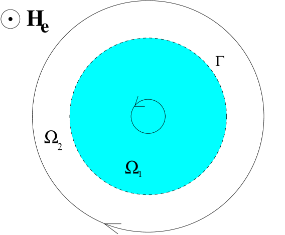
FIG. 1.: The sample cross-section is divided into two subdomains by the circle $\Gamma$. The arrows indicate the direction of the current.

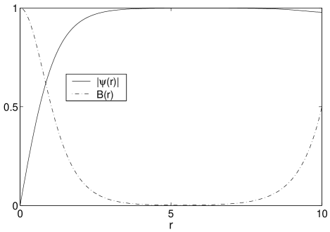
FIG. 2.: Behaviour of the order parameter and the magnetic field at the dual point for a cylinder of radius 10 $\lambda\sqrt{2}$ containing one vortex.

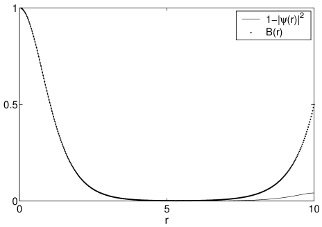
FIG. 3.: Comparison between $B$ and $1-|\psi|^{2}$ in a cylinder of radius 10 $\lambda\sqrt{2}$ containing one vortex.

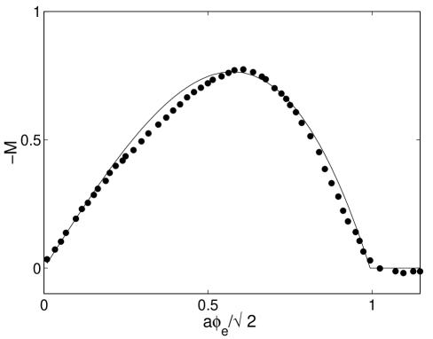
FIG. 4.: Magnetization of a fractional fluxoid disk. Comparison between the experimental measurements [8]  (for $R=0.31\mu m$) and the theoretical curve taken from the expression (45).

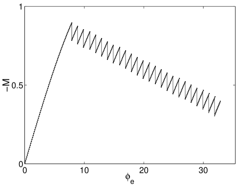
FIG. 5.: Behaviour of the magnetization of a disk with radius 10 $\lambda\sqrt{2}$, at the dual point. Dots represent the numerical solution and the solid curve the expression (14) together with (32). The only free parameter $\delta$ has been taken to $\delta=0.76\lambda$.

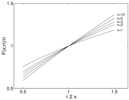
FIG. 6.: Behaviour of the free energy per vortex $F/n={\cal F}/2\pi n$ as a function of $\sqrt{2}\kappa$ for different values of $n$, the number of vortices. At the self-dual point $\sqrt{2}\kappa=1$, the energy ${\cal F}(n)=n{\cal F}(1)$ so that the interaction energy between the vortices vanishes identically.

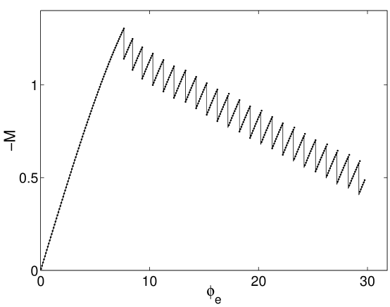
FIG. 7.: Magnetization curve of a disk of radius 10 $\lambda\sqrt{2}$, as a function of the applied field for $\kappa{\sqrt{2}}=0.9$. Dots represent the numerical solution and the solid curve the expression (14) together with (54, 51). The only free parameter $\delta$ has been taken to $\delta=0.76\lambda$.

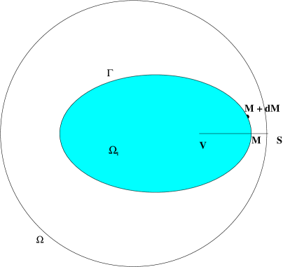
FIG. 8.: The separation of a system without cylindrical symmetry in two subdomains by a curve $\Gamma$.

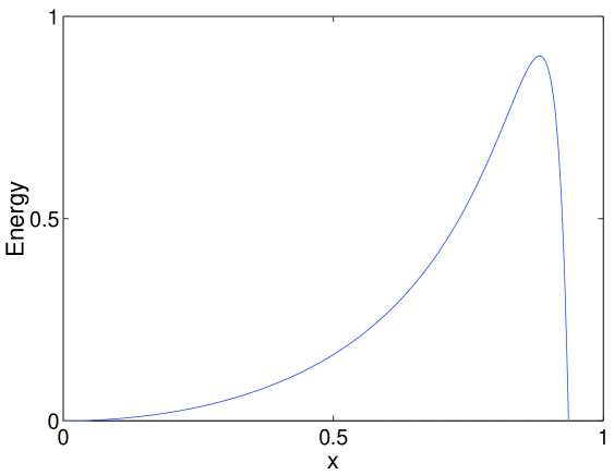
FIG. 9.: Confining energy of a vortex inside a disk due to edge currents.

n	$\alpha(n)$	n	$\alpha(n)$	n	$\alpha(n)$
1	0.417	11	0.785	21	0.841
2	0.544	12	0.794	22	0.845
3	0.613	13	0.802	23	0.847
4	0.658	14	0.809	24	0.850
5	0.690	15	0.815	25	0.853
6	0.715	16	0.821	26	0.855
7	0.734	17	0.826	27	0.857
8	0.750	18	0.830	28	0.859
9	0.764	19	0.834	29	0.860
10	0.775	20	0.838	30	0.862

TABLE I.: The numerical values of the function $\alpha(n)$ for $n$ ranging from $1$ to $30$.

REFERENCES

- [1] A.K. Geim, I.V. Grigorieva, S.V. Dubonos, J.G.S. Lok, J.C. Maan, A.E. Filippov and F.M. Peeters, Nature, 390, 259 (1997)
- [2] K.W. Madison, F. Chevy, W. Wohlleben and J. Dalibard, to appear in Phys.Rev.Lett cond-mat/9912015
- [3] A.K. Geim, S.V. Dubonos, J.G.S. Lok, I.V. Grigorieva, J.C. Maan, L. Theil Hansen and P.E. Lindelof, Appl.Phys.Lett. 71, 2379 (1997).
- [4] A.K. Geim, S.V. Dubonos, J.G.S. Lok, M. Henini and J.C. Maan, Nature, 396, 144 (1998)
- [5] V.V. Moshchalkov, L. Gielen, C. Strunk, R. Jonckheere, X. Qiu, C. Van Haesendonck and Y. Bruynseraede, Nature, 373, 319 (1995)
- [6] O. Buisson, P. Gandit, R. Rammal, Y.Y. Wang and B. Pannetier, Phys.Lett.A, 150, 36 (1990)
- [7] P. Singha Deo, F.M. Peeters and V.A. Schweigert, submitted to Superlattices and microstructures (1999) cond-mat/9812193
- [8] P. Singha Deo, V.A. Schweigert, F.M. Peeters and A.K. Geim, Phys.Rev.Lett. 79, 4653 (1997)
- [9] P. Singha Deo, V.A. Schweigert and F.M. Peeters Phys. Rev. B 59, 6039 (1999)
- [10] J.J. Palacios, Phys. Rev. B 58, R5948 (1998)
- [11] J.J. Palacios, cond-mat/9908341
- [12] V.A. Schweigert, P. Singha Deo and F.M. Peeters, Phys.Rev.Lett. 81, 2783 (1998)
- [13] P.G. de Gennes, Superconductivity of metals and alloys Addison-Wesley (1989)
- [14] W. A. Little and R.D. Parks, Phys.Rev.Lett. 9, 9 (1962)
- [15] R. P. Groff and R.D. Parks, Phys.Rev 176, 567 (1968)
- [16] R. Benoist and W. Zwerger, Z.Phys. B 103, 377 (1997)
- [17] G. Böbel, Nuovo Cimento 38, 6320 (1965)
- [18] E.A. Shapoval, JETP Letters 69, 577 (1999)
- [19] J. Pearl, Appl. Phys. Lett. 5, 65 (1964)
- [20] A.L. Fetter, Phys. Rev. B 22, 1200 (1980)
- [21] C.P. Bean and J.D. Livingston, Phys.Rev.Lett. 12, 14 (1964)
- [22] A.S. Krasilnikov, L.G. Mamsurova, N.G. Trusevich, L.G. Shcherbakova and K.K Pukhov, Supercond.Sci.Technol 8, 1 (1995)
- [23] P.A. Venegas and E. Sardella, Phys. Rev. B 58, 5789 (1998)
- [24] D. Saint-James, E.J. Thomas and G. Sarma, Type II Superconductivity Pergamon Press (1969)
- [25] E.B. Bogomol’nyi, Sov.J.Nucl.Phys. 24, 449 (1977)
- [26] V.A. Schweigert and F.M. Peeters, Phys.Rev.Lett. 83, 2409 (1999); V.A. Schweigert and F.M. Peeters, cond-mat/9910110
- [27] J.L. Harden and V. Arp, Cryogenics 3, 105 (1963)
- [28] E. Akkermans and K. Mallick J. Phys. A. 32, 7133 (1999)
- [29] L. Jacobs and C. Rebbi, Phys.Rev. B 19, 4486 (1979)
- [30] F. London, Superfluids, Vol. 1: Macroscopic theory of superconductivity Dover (1960)
- [31] G. Dunne, private communication.
- [32] E. Akkermans and K. Mallick, proceedings of Les Houches Summer School Topological Aspects of Low dimensional systems (1999) cond-mat/9907441
- [33] V.A. Schweigert and F.M. Peeters, Phys.Rev B 57, 13817 (1998)
- [34] E. Akkermans, D. Gangardt and K. Mallick, in preparation
- [35] E.B. Bogomol’nyi and A.I. Vainshtein, Sov.J.Nucl.Phys 23, 588 (1976)
- [36] A.T. Dorsey, Ann.Phys, 233, 248 (1994)
- [37] G.S. Lozano, M.V. Manias and E.F. Moreno, cond-mat/0005199
- [38] W.H. Press, B.P. Flannery, S.A. Teukolsky and W.T. Vetterling, Numerical Recipes: The Art of Scientific Computing Cambridge University Press, (1992)