Phase field under stress

A phase-field approach describing the dynamics of a strained solid in contact with its melt is developed. Using a formulation that is independent of the state of reference chosen for the displacement field, we write down the elastic energy in an unambiguous fashion, thus obtaining an entire class of models. According to the choice of reference state, the particular model emerging from this class will become equivalent to one of the two independently constructed models, on which brief accounts have been given recently [J. Müller and M. Grant, Phys. Rev. Lett. 82, 1736 (1999); K. Kassner and C. Misbah, Europhys. Lett. 46, 217 (1999)]. We show that our phase-field approach recovers the sharp-interface limit corresponding to the continuum model equations describing the Asaro-Tiller-Grinfeld instability. Moreover, we use our model to derive hitherto unknown sharp-interface equations for a situation including a field of body forces. The numerical utility of the phase-field approach is demonstrated by reproducing some known results and by comparison with a sharp-interface simulation. We then proceed to investigate the dynamics of extended systems within the phase-field model which contains an inherent lower length cutoff, thus avoiding cusp singularities. It is found that a periodic array of grooves generically evolves into a superstructure which arises from a series of imperfect period doublings. For wavenumbers close to the fastest-growing mode of the linear instability, the first period doubling can be obtained analytically. Both the dynamics of an initially periodic array and a random initial structure can be described as a coarsening process with winning grooves temporarily accelerating whereas losing ones decelerate and even reverse their direction of motion. In the absence of gravity, the end state of a laterally finite system is a single groove growing at constant velocity, as long as no secondary instabilities arise (that we have not been able to see with our code). With gravity, several grooves are possible, all of which are bound to stop eventually. A laterally infinite system approaches a scaling state in the absence of gravity and probably with gravity, too.

PACS numbers: 81.10.Aj, 05.70.Ln, 81.40.Jj, 81.30.Fb

I Introduction

Already when introducing the notion of a surface quantity Gibbs implicitly entertained the idea of a phase field $\phi$: any density of an extensive quantity (e.g., the mass density) between two coexisting phases changes gradually (but swiftly) from its value in one phase to its value in the other. The existence of a transition zone, though microscopically of atomic extent (far enough from a second-order phase transition), underlies the very Gibbs definition of surface quantities. In phase transition phenomena, either of first or second order, this notion has been adopted in Landau’s spirit. Because energy is an extensive quantity, too, there is an extra energetic cost associated with the transition region, characterized in the appropriate thermodynamical potential density by a term of the form $\epsilon^{\ast}(\nabla\phi)^{2}$, $\epsilon^{\ast}$ being the stiffness of the transition region.

The notion of a phase field has appeared abundantly in the literature in the context of phase transition phenomena[1, 2, 3]. The transition width diverges for a second-order phase transition at the critical point, and thus it is essential to introduce the transition region. For a first-order transition, such as a liquid-solid interface, confering an importance to the interface thickness may seem quite anecdotic if one is interested in properties which occur on a scale larger than the atomic one; typical examples are dendritic patterns occuring at the scale of a $\mu m$. Nevertheless, it is here, where phase-field modeling has become most useful in numerical treatments.

Before phase-field models became popular, it seemed quite natural to treat the surface as a geometric location on which boundary conditions are imposed (e.g., for a moving front the normal velocity is proportional to the jump in the gradient of the temperature or concentration field). This is the so-called sharp interface approach, adopted both in analytical and numerical studies in a variety of contexts of front problems.

There has been an upsurge of interest in the phase-field approach to free-boundary problems more recently, though the method was actually introduced pretty early [4, 5], as a computational tool to model solidification. Various studies[6, 7, 8, 9, 10, 11] have demonstrated the virtues of this method in moving-boundary problems.

Regarding the way how to use phase-field models, there are two distinctly different philosophies. These may be best discussed considering dendritic growth, where a set of well-established continuum equations exists describing phenomena in terms of a sharp interface. On the basis of this knowledge, a phase-field model can be justified by simply showing that it is asymptotic to the correct sharp-interface description, i.e., that the latter arises as the sharp-interface limit of the phase-field model when the interface width is taken to zero. This is definitely a sufficient condition for the phase-field model to yield a correct description of the continuum limit, providing the interface thickness is taken small enough. Small enough sometimes may mean impractically small. The second approach to phase-field modeling is to guess or derive an appropriate form for the free energy of the two-phase system, including the energy cost of the transition region and to regard this as a physical model in its own right. In this case, one might actually forgo considering the limit of small interface thickness and such a model would even make sense, if the strict limit of vanishing interface width did not correspond to sensible physics.

Of course, a problem arises, if a phase-field model obtained in the second way gives predictions that are different from that of the sharp-interface equations. A follower of the first philosophy would then discard the phase-field model, whereas one of the second might contemplate the possibility that his model contain more physics than the sharp-interface model. In the case of dendritic growth the situation is pretty clear: the sharp interface model gives the right answers. However, this statement cannot be generalized easily, since not all sharp-interface models are as well-founded as that for dendritic growth and because the extreme smallness of the interface width cannot be always guaranteed (it might for example become doubtful for a phase transition that is only weakly first order).

A related issue is the question of thermodynamic consistency, i.e., the derivation of the model in the spirit of Gibbs from a free-energy or entropy functional. It is clear that with a known sharp-interface limit in mind, there is no need at all to obtain a phase-field model this way (which would mean to make it “thermodynamically consistent”) as long as one ensures its asymptotic approach to this limit. In fact, it has turned out that in some cases where both a thermodynamically consistent formulation of a phase-field model and a nonvariational formulation exist, the latter was numerically more efficient [12] and hence preferable on practical grounds.

On the other hand, thermodynamic consistency has its virtues. This can be seen particularly well in the case considered here, the influence of elasticity on the stability of a solid interface. It is quite straightforward to write down the contribution of the elastic energy to the total free energy. Hence, if we have a good idea about the physical origin of the free energy to be considered, the corresponding phase-field model is easily obtained, and it is bound to be right. As a result, one may derive sharp-interface equations in cases where they are not known.

For the Grinfeld instability to be considered here, the sharp-interface equations are well known. Nevertheless, it is of course tremendously satisfying, if they simply pop out of the phase-field equations as the sharp-interface limit. Not only does this provide a natural countercheck of our ansatz for the free energy, but it also gives us a new angle of view at the instability, leading to the prediction of circumstances in which the Grinfeld instability should not occur under anisotropic stress, but might appear with isotropic stress. We shall consider this point in section II.

Let us return to the advantages of the phase-field method. The first virtue of phase fields is pretty obvious: instead of tracking permanently the a priori unknown interface position in the sharp-interface limit, and imposing nontrivial boundary conditions for the discontinuity of the fields, the interface in the phase-field approach is nothing but the location of a rapid variation of the field $\phi$, while the two phases are treated as the same entity. Thus there is no boundary condition to be imposed in the transition region, a fact which greatly facilitates both the numerical implementation and analysis. This is done at some price: one must, in principle, mix disparate length (and thus time) scales: the pattern length and the interfacial width, whose ratio may range over many orders of magnitude. This may render the numerical procedure excessively expensive, a fact which would quickly take us back to the sharp-interface problem, where the small length scales out of the problem.

As discussed recently[13], the sharp-interface limit that one would like to represent when writing the phase-field equations, only makes physical sense on “outer” length scales much larger than the physical extent $l_{c}$ of the transition region, and thus does not depend structurally on the details of the interface shape on the inner $l_{c}$ scale. The mathematical question, formulated in the framework of phase-field models, of formally recovering the sharp interface description via an asymptotic (multi-scale) expansion in the limit $l_{c}\rightarrow 0$ might, from this point of view, seem irrelevant.

It should however be kept in mind that the actual matching conditions are imposed for the limit, where an “inner” variable (defined in the transition region) goes to infinity. This entails a certain amount of liberty in the choice of functions defining the free-energy density, because the precise behavior of these functions on the inner scale does not matter. Hence, the validity of a phase-field model can indeed be judged by simply showing that it asymptotically reproduces the correct sharp-interface description. Whether the additional information encoded in the structure of the phase-field model on the inner scale is physically relevant, is a question to be decided on a case by case basis (as implied by our discussion above).

An example where this is relevant, is provided by the Young condition for the contact angle of a droplet on a substrate. This is a condition on “outer” scales, while the inner scale is rather governed by van der Waals interactions of a thin liquid film with the substrate, leading to some nontrivial corrections of the wetting profile at small atomic length scales. In other words, what matters in the phase-field description is not that the width of the interface be of atomic extent, but rather that it be small in comparison with the scale of the pattern of interest.

This physical argument has been cast in a mathematical form in [12], where the thin-interface limit was considered, arising from an alternative asymptotic procedure. This has to be contrasted with the sharp-interface limit with the small parameter being the ratio of the interface thickness to the capillary length. Making the width of the interface small only in comparison with the scale of the pattern leads to a rather important enhancement of the computing speed, thus rendering the phase-field approach attractive with regard to numerical efficiency as well. Unfortunately, in most systems the thin-interface limit is not as easily accessible as for dendritic growth in the thermal model [12]. Hence, it is difficult in general to make our argument mathematically rigorous. However, we will give a consideration of length scales in section II that clarifies what are the ratios that have to be kept small for our model to be a good description. Moreover, we have checked that the dependence of the results on the interface width becomes weak for the small values that we use for the latter.

Finally the phase-field approach has the additional virtue of regularizing instabilities, such as the development of cuspy structures, often setting severe limitations in numerical studies. In the elastic system, we are led to the question whether the sharp-interface models still make sense in the limit where they predict finite-time singularities. No such singularities arise in the phase-field model, thus possibly extending the range of validity of the latter beyond that of the former. This will be discussed in more detail in section IV.

In the context of growth phenomena phase-field approaches have been introduced in problems involving temperature or concentration fields. There are myriads of situations, however, where the corresponding transition is monitored, or at least affected, by strain. A typical situation is a solid under uniaxial stress. This leads to the Asaro-Tiller-Grinfeld (ATG) instability [14, 15] (see Ref. [16] for a recent review. A surface corrugation allows to lower the stored elastic energy. Other examples of particular interest include solid-solid transformations, phases in nonequilibrium gels, molecular beam epitaxy, solidification of lava, etc. It is thus highly desirable to develop a phase-field approach including the stress as an active variable. Very recently, two groups, Müller-Grant (MG) and Kassner-Misbah (KM) [17, 18], have independently developed such an approach and have given a brief account on it.

This paper will present extensive discussions of this question and give new results. We shall also provide a comparison between the MG and KM models, and point out similarities and dissimilarities. As already known from sharp-interface simulations[19, 20] a solid under stress presents a somehow stringent behavior in that no stable steady-state solution seems to exist. This is also the case from analytical studies in the long-wavelength limit[21]. Nozières had shown [22] that the bifurcation from the planar front to the deformed one is subcritical (the analogue of a first-order transition). The study of Spencer and Meiron [23] focused on structures with a given basic wave number in the absence of gravity (where the instability does not have a threshold) and on systems, in which the transport mechanism necessary for the instability to manifest itself is surface diffusion. They find that in the unstable range of wavenumbers (i.e., for wavenumbers below the marginal value, above which surface tension stabilizes the planar interface) there exist finite-amplitude steady-state solutions, if the wavenumber is close enough to marginal. This branch of steady-state solutions terminates by structures developing cusp singularities, despite the stabilizing influence of surface tension. It cannot be overemphasized that this result is not an artifact of their numerics. Indeed, they investigate carefully the effects of numerical fine-graining using a code with spectral accuracy, and their discretization sequence seems to get fine enough to render their extrapolation valid. The evidence for the appearance of true cusps in the sharp-interface continuum model becomes compelling, if one takes into account the work of Chiu and Gao [24] who found analytical solutions developing cusp singularities in finite time. The conclusion of Spencer and Meiron is that for generic initial conditions, including sufficiently small wavenumbers, finite-time singularities will always occur. Moreover, they state that this is also true in the presence of gravity (beyond the threshold) and under fairly general conditions.

For a physical system, finite-time singularities will be prevented by intervening effects that are not considered in the model. This would mean that nonlinear elasticity and plasticity have to be taken into account. For example, the formation of dislocations (plasticity) could blunt cusps again.

Two questions then arise. What kind of structures can be expected before cusp formation and what kind of structures will prevail eventually? Our previous study[20] has shown that the initial cellular pattern may develop into a super-structure, where a groove or several of them accelerate in a spectacular fashion, thus relieving the stresses in their surroundings significantly and causing nearby grooves to recede. Further evolution of the structure was difficult to handle numerically, due to the development of cusps which appear in the numerics as they should according to the analytic results [24]. In the phase-field approach presented here, no cusps can arise. The question is of course legitimate, whether the model, which allows to track the dynamics of the structure much beyond the times where earlier studies had to fail numerically, still gives a faithful description of the physics. Here we take the point of view, that the details of the description in the locations, where stresses become large, may not be correctly captured by the model, since we neither include nonlinear elastic effects nor other effects such as capillary overpressure explicitly [25]. If they have the right sign, these might prevent cusp formation [23]. However, the result of any such effect must be to blunt cusps, which the phase-field model does. As we shall see, it does so in a non-obtrusive way by introducing a cutoff for interface curvature. Moreover, away from the cusps, stresses are low enough for linear elasticity to apply. Hence, we believe that the development of the overall morphology is still correctly described by the phase-field model.

A more detailed justification would point out that nonlinear elasticity will first make itself felt by stresses increasing more slowly as a function of strains than in the linear case and that next plasticity will act to introduce an upper cutoff for stresses, where the material will yield. Now the effect of any resulting modification in the stress-strain relationship on the remaining body can be reproduced by cutting out the piece of material where linear elasticity ceases to hold and by requiring boundary conditions at the edge of the cut-out piece that correspond to the correct stresses. In the case of material yielding near a singularity of the stress field (obtained assuming linear elasticity), these boundary conditions will essentially be that the stresses are close to the yield stress at the boundary. This is mimicked by the phase-field model in which the maximum supportable stress is, for a given geometry, determined by the interface width.

Therefore, we think this is one case, where the phase-field model can do more in the description of the physical system than its sharp-interface limit.

It will emerge that usually one leading groove continues to deepen while neighboring ones recede after the winner has started to relieve the stress that kept them growing. Finally the surface shows a single deep groove evolving in time and becoming a location of a strong stress accumulation, possibly until the fracture threshold is reached. Presumably, before that stage is reached the validity of the model will break down. We shall make some speculation on future directions to elucidate the physical behavior in real systems. For generic initial conditions, we may consider the dynamics a continual coarsening process which initially develops as described in [17] and later is dominated by groove growth and shrinkage.

The paper is organized as follows. In section II we give the continuum equations ordinarily used in the description of the Grinfeld instability. This is mainly done in order to introduce appropriate length and time scales in nondimensionalizing the equations; then we present our phase-field approach and discuss how the interface width has to be chosen in comparison with the other length scales. We demonstrate how the phase-field model can be employed to derive new sharp-interface equations in the presence of body forces breaking rotational invariance.

Section III presents validation results, a comparison of the MG and KM models and describes the main findings of our simulations. Section IV sums up the results and discusses perspectives. The mathematically rigorous asymptotic expansion used to derive the sharp-interface limit has been relegated to an appendix, as the calculation is somewhat lengthy and would interrupt the flow of the text. Since we use the MG model in a slightly different form from that presented originally [17], we give the connection between the two formulations in a second appendix. Finally, appendix C contains the analytic derivation via conformal mapping of the stresses for a particular interface shape to be compared with the numerics.

II The Grinfeld instability

A Sharp-interface equations

A description of the basic ingredients of the Grinfeld instability has been given elsewhere [16]. Therefore, we may restrict ourselves to explaining the physical mechanism and giving the equations.

We wish to describe the behavior of a solid submitted to uniaxial stress, at the surface of which material transport is possible. Consider the example of a solid in contact with its melt. An accidental corrugation of the surface will act to reduce the stress at its tip and increase it in the valleys next to it. That is, the solid can decrease its elastic energy density by growing tips (where the stress is lower) and by increasing the depths of valleys (where it gets rid of material having a higher density of elastic energy due to larger stresses). This tendency is most easily cast into equations by writing down the chemical potential difference $\Delta\mu=\mu_{s}-\mu_{\ell}$ at the interface (the subscripts refer to the solid and liquid or nonsolid phases, respecively) [20]:

$$\Delta\mu={1-\nu^{2}\over 2E\rho_{s}}(\sigma_{tt}-\sigma_{nn})^{2}+\frac{1}{\rho_{s}}\gamma\kappa+\frac{\Delta\rho}{\rho_{s}}g\zeta(x)$$ (1)

Herein, the first term is of elastic origin; $\sigma_{tt}$ and $\sigma_{nn}$ are the normal stresses tangential and perpendicular to the interface, $E$ is Young’s modulus, $\nu$ the Poisson number, and $\rho_{s}$ the density of the solid. The second term describes the stabilizing influence of the surface stiffness $\gamma$, taken isotropic here (so it becomes identical to the surface energy). $\kappa$ is the curvature of the interface; for simplicity, we consider the two-dimensional case only. Finally, the third term is the contribution of gravity ($g$), where $\Delta\rho=\rho_{s}-\rho_{\ell}$ is the density contrast between the solid and the liquid (or vacuum) and $\zeta(x)$ is the interface position, given by its $z$ coordinate (the $z$ axis is oriented antiparallel to the gravitational force). Equation (1) holds for plane strain. For plane stress, the prefactor $1-\nu^{2}$ has to be dropped.

The dynamics is then described by giving the normal velocity in terms of the chemical potential difference. For a solid in contact with its melt this would simply be

$$v_{n}=-\frac{1}{k}\Delta\mu\>,$$ (2)

where $k$ is an inverse mobility with the dimension of a velocity. In the case of a solid in contact with vacuum and surface diffusion as the prevailing transport mechanism we would have $v_{n}=D\nabla^{2}\Delta\mu$ instead.

Of course, in order to compute $v_{n}$, we must first obtain the stresses entering (1). This involves solving an elastic problem ($\partial_{j}\sigma_{ij}=0$) with a prescribed external stress and boundary conditions on the interface, assuming an appropriate constitutive law. Ordinarily, Hooke’s law for isotropic elastic bodies is assumed [therefore we have only two elastic constants in (1)]. Neglecting the capillary overpressure, which usually is a good approximation, we have as boundary conditions at the interface $\sigma_{nn}=-p$, where $p$ is the pressure in the second phase, and $\sigma_{nt}=0$, i.e., the shear stress vanishes.

A linear stability analysis of a planar interface under the dynamics given by equations (1) and (2) yields the following dispersion relation ($\omega$ is the growth rate, $q$ the wave number)

$$\omega=\frac{1}{k\rho_{s}}\left\{{2\sigma_{0}^{2}({1-\nu^{2}})\over E}q-\gamma q^{2}-\Delta\rho g\right\}\>.$$ (3)

$\sigma_{0}$ is the uniaxial external stress. Eq. (3) provides us with a critical wave number $q_{c}=\sqrt{\Delta\rho g/\gamma}$ (an inverse capillary length) and a critical stress $\sigma_{0c}=\left[\gamma q_{c}E/(1-\nu^{2})\right]^{\frac{1}{2}}$, below which the planar interface is stable. The wave number of the fastest-growing mode can be inverted to give a length

$$\ell_{1}=\frac{\gamma E}{\sigma_{0}^{2}(1-\nu^{2})}\>.$$ (4)

Apart from a prefactor of $2/\pi$, this length is identical to the so-called Griffith length.

Note that a planar interface will not remain at its original equilibrium position, even when only a subthreshold stress is applied, i.e., when it is “stable”. Our dynamical equations predict that it has a nonzero velocity as long as $\Delta\mu$ is different from zero. Hence it will recede to smaller values of $\zeta$. If the density of the solid is bigger than that of the liquid, the chemical potential on the solid side of the receding interface decreases faster than that on the liquid side and there is a new equilibrium position, which can be computed directly from (1) and which evaluates to

$$\Delta\zeta\equiv-\ell_{2}=-\frac{1-\nu^{2}}{2\Delta\rho gE}\sigma_{0}^{2}\>.$$ (5)

Equations (4) and (5) provide us with two independent length scales of the problem, the first of which is due to a competition between stress and surface energy, while the second arises from the competition between stress and gravity. For the purpose of nondimensionalizing equations, $\ell_{1}$ is more appropriate, as this length does not diverge in the limit of vanishing density difference (or gravity). To obtain a natural time scale $\tau$, we can replace $q$ in either of the two wave-number dependent terms of (3) by $1/\ell_{1}$. This leads to

$$\tau=\frac{k\rho_{s}\gamma E^{2}}{\sigma_{0}^{4}(1-\nu^{2})^{2}}\>.$$ (6)

The nondimensional version of the dispersion relation then reads ($\tilde{\omega}=\tau\omega$, $\tilde{q}=\ell_{1}q$):

$$\tilde{\omega}=2\tilde{q}-\tilde{q}^{2}-\frac{\ell_{1}}{2\ell_{2}}\>,$$ (7)

which shows clearly that the problem without gravity (when $\ell_{2}$ becomes infinite) can be made parameter free, i.e., elastic and other parameters only set the time and length scales; apart from that we should expect the same dynamics for all systems. With gravity, the dynamics is essentially determined by the ratio of the two length scales introduced.

B Elastic energy and state of reference

Let us now proceed to investigate the contributions to the free energy of the same system. The phase-field model will then consist in writing the free-energy density that takes into consideration the global elastic energy in both phases.

As is usual with elastic problems, it is important to specify the state of reference defining the positions of material particles with respect to which displacements are measured. This is crucial whenever the reference state is not that of an undeformed body but one that is subject to prestraining (which will turn out useful later). In order to make this point clear, and in the hope of helping subsequent discussions, we would like first to dwell on this issue.

If the only energy present is elastic energy and Hooke’s law holds true, the free energy per unit volume can be written as

$$f=\mu\,u_{ij}u_{ij}+{\lambda\over 2}u_{ii}^{2}\>,$$ (8)

where summation over double subscripts is implied. $\lambda$ and $\mu$ are the Lamé constants, $\mu$ being better known as the shear modulus. For plane strain, these elastic constants are related to Young’s modulus and the Poisson ratio via $\mu=E/[2(1+\nu)]$ and $\lambda=E\nu/[(1+\nu)(1-2\nu)]$. The stress tensor $\sigma_{ij}$ is then

$$\sigma_{ij}=\frac{\partial f}{\partial u_{ij}}=2\mu u_{ij}+\lambda u_{kk}\delta_{ij}=2\mu(u_{ij}-u_{kk}\frac{\delta_{ij}}{d})+Ku_{kk}\delta_{ij}\>.$$ (9)

$K=2\mu+\lambda/d$ is the bulk modulus, and the last relation has the advantage of making explicit the parts of the stress tensor causing pure shape and pure volume changes, respectively. ($d$ is the spatial dimension.) We will nevertheless mainly use the relations containing $\mu$ and $\lambda$, which are more compact. The implied reference state here is $u_{ij}=0$, for which $\sigma_{ij}=0$.

However, if we choose a reference state given by a different strain tensor $u_{ij}^{(0)}$, setting $\tilde{u}_{ij}=u_{ij}-u_{ij}^{(0)}$, then we should not simply replace $u_{ij}$ by $\tilde{u}_{ij}$ in (9), as the stress tensor and the elastic energy are, in principle, measurable quantities and should thus be unaffected by a change of strain reference state. Hence, we have to write

$$\sigma_{ij}=2\mu\left(\tilde{u}_{ij}+u_{ij}^{(0)}\right)+\lambda\left(\tilde{u}_{kk}+u_{kk}^{(0)}\right)\delta_{ij}\>,$$ (10)

and change definition (8) accordingly, i.e. replace $u_{ij}$ by $\tilde{u}_{ij}+u_{ij}^{(0)}$. In this situation, the zero-strain state would not be stress-free. An alternative way to specify a reference state would then consist in giving the stress of the zero-strain state.

In general, the thermodynamic system under consideration will not only contain elastic contributions. Then the equilibrium state, corresponding to a minimum of the free energy, may not be a state of vanishing strain. A trivial example is a solid in equilibrium with its melt, where the equilibrium state in the solid corresponds to the strain produced by the equilibrium pressure $p$ of the liquid (the equilibrium stress tensor of the solid is $-p\delta_{ij}$). The form of the free-energy density accounting for such a situation is not (8) [which does not exhibit a minimum at $u_{ij}^{({\rm eq})}\neq 0$] but

$$f=\mu\left(u_{ij}-u_{ij}^{({\rm eq})}\right)\left(u_{ij}-u_{ij}^{({\rm eq})}\right)+{\lambda\over 2}\left(u_{ii}-u_{ii}^{({\rm eq})}\right)^{2}\>.$$ (11)

This is manifestly minimum at $u_{ij}^{({\rm eq})}$ and the nonzero value of the latter quantity takes into account nonelastic contributions to the free energy. If we now define the stress from the first relation in Eq. (9), i.e., $\sigma_{ij}=\partial f/\partial u_{ij}$, it will be nonzero only, if there are forces driving the system away from equilibrium. If we rather define it via the second equality of Eq. (9), meaning that we set $\sigma_{ij}=2\mu u_{ij}+\lambda u_{kk}\delta_{ij}$ (which is now different from $\partial f/\partial u_{ij}$), it will describe, in addition to these forces the prestress necessary to keep the system in equilibrium. An invariant relation between stresses and strains follows from requiring

$$f=\int_{u_{ij}^{({\rm eq})}}^{u_{ij}}\left(\sigma_{ij}-\sigma_{ij}^{({\rm eq})}\right)du_{ij}\>,$$ (12)

which leads to

$$\sigma_{ij}-\sigma_{ij}^{({\rm eq})}=2\mu\left(u_{ij}-u_{ij}^{({\rm eq})}\right)+\lambda\left(u_{kk}-u_{kk}^{({\rm eq})}\right)\delta_{ij}\>.$$ (13)

Once both $\sigma_{ij}^{({\rm eq})}$ and $u_{ij}^{({\rm eq})}$ are specified, this equation gives us an unambiguous relationship between stresses and strains. Depending on which variables we choose to define the reference state, we obtain the conjugate variables of the same state from (13). If we choose, for instance, a strain-free state as reference, this equation will provide us with the corresponding stress of reference, if we choose a stress-free state of reference, it will yield the strain of reference.

As an example we can look at a case where the equilibrium stress is $\sigma_{ij}^{({\rm eq})}=-p_{0}\delta_{ij}$, and ask what should the strain be. Hooke’s law – written in a such a way that the absence of strain implies the absence of stress as well [see (9)] – then gives us an equilibrium strain

$$u_{ij}^{({\rm eq})}=-{p_{0}\over 2\mu+\lambda d}\delta_{ij}\>.$$ (14)

Since the free energy must not depend on the choice of reference state, it is clear that it does not matter whether we use ${u}_{ij}$ or $\tilde{u}_{ij}$ in (13), providing that we use the correct values of $u_{ij}^{({\rm eq})}$ and $\tilde{u}_{ij}^{({\rm eq})}$, respectively. Suppose that we choose another reference state characterized by the strain tensor $\tilde{u}_{ij}$ in such a way that when the strain is zero, the stress is equal to $-p_{0s}\delta_{ij}$. A vanishing strain then corresponds to a pre-stressed situation. If the equilibrium stress is again $-p_{0}\delta_{ij}$ as above, we must have a new equilibrium strain $\tilde{u}_{ij}^{({\rm eq})}$ obeying, according to our invariant relation (13), $-p_{0s}\delta_{ij}+p_{0}\delta_{ij}=-2\mu\tilde{u}_{ij}^{({\rm eq})}-\lambda\tilde{u}_{kk}^{({\rm eq})}\delta_{ij}$. After a simple manipulation we obtain

$$\tilde{u}_{ij}^{({\rm eq})}={p_{0s}-p_{0}\over 2\mu+\lambda d}\delta_{ij}$$ (15)

Of course, Eq. (14) is a special case of (15) for $p_{0s}=0$. The free energy, expressed by $\tilde{u}_{ij}$, then reads

$$f = \mu(\tilde{u}_{ij}-\tilde{u}^{(\rm eq)}_{ij})(\tilde{u}_{ij}-\tilde{u}^{(\rm eq)}_{ij})+{\lambda\over 2}(\tilde{u}_{ii}-\tilde{u}^{(\rm eq)}_{ii})^{2}$$ (16)

$$= \mu\tilde{u}_{ij}\tilde{u}_{ij}+{\lambda\over 2}\tilde{u}_{ii}\tilde{u}_{jj}+(p_{0}-p_{0s})\tilde{u}_{ii}+{d\over 2(2\mu+\lambda d)}(p_{0}-p_{0s})^{2}$$ (17)

It should be realized that Eqs. (11) and (17) describe exactly the same situation, if corresponding values for the strain fields without and with a tilde are inserted. At this point we have said nothing about applied external stresses or so. However, if we choose, say, vanishing displacement as boundary condition at a planar interface, directed along the $x$ direction, then this will correspond to two different physical situations for the two different choices of the state of reference. Let us for simplicity assume $p_{0}=0$. According to (14), we then have $u^{(\rm eq)}_{ij}=0$, and (11) implies (8). Setting $u_{xx}=0$ in Eq. (9) we obtain, because of the boundary condition $\sigma_{zz}=0$ that also $u_{zz}=0$, and there is no stress at all. On the other hand, if we set $\tilde{u}_{xx}=0$, we have to use (13) and (15) to obtain the elastic state of the solid. The boundary condition for $\sigma_{zz}$ implies $u_{zz}=p_{0s}/(2\mu+\lambda)$, which in turn leads to $\sigma_{xx}=-2\mu p_{0s}/(2\mu+\lambda)$; hence vanishing displacement along our planar interface means a solid that is homogeneously strained in the $x$ direction with a prestress $\sigma_{0}=\sigma_{xx}$.

As we shall see later, the latter choice of the state of reference has been made in the phase-field model discussed in [17], the former (setting $p_{0s}=0$) in [18]. These are the most natural choices, although an infinity of (less natural) alternatives is available.

C The phase-field model

The total (solid+liquid) free energy of the system can be written as

$$F[\phi,\;\{u_{ij}\}]=\int dV\left[f(\phi,\,\{u_{ij}\})+{1\over 2}\Gamma\epsilon^{2}({\bf\nabla}\phi)^{2}\right]$$ (18)

where $\epsilon$ is a length parameter controlling the order of magnitude of the transition region described by the phase field. $\Gamma=3\gamma/\epsilon$ is the energy density corresponding to the surface energy $\gamma$ being distributed over a layer of width $\approx\epsilon$. (The factor 3 is just a convenient choice, simplifying later derivations.)

If we start from the invariant form (13), we can set up a whole class of phase-field models at once and specify the reference state later. In order to be able to write a single elastic energy expression for the two-phase system, we formally treat the liquid as a shear-free solid (not including hydrodynamics). We will discuss some consequences of this approach later.

A straightforward ansatz for the elastic energy density is then

$$f_{{\rm el}}(\phi,\{u_{ij}\}) = h(\phi)f_{{\rm sol}}(\{u_{ij}\})+[1-h(\phi)]f_{{\rm liq}}(\{u_{ij}\})$$ (19)

$$= h(\phi)\left\{\mu\left(u_{ij}-u_{ij,s}^{({\rm eq})}\right)\left(u_{ij}-u_{ij,s}^{({\rm eq})}\right)+{\lambda\over 2}\left(u_{ii}-u_{ii,s}^{({\rm eq})}\right)^{2}\right\}$$ (21)

$$\mbox{}+\left[1-h(\phi)\right]{\tilde{\lambda}\over 2}\left(u_{ii}-u_{ii,\ell}^{({\rm eq})}\right)^{2}\>,$$

where $f_{{\rm sol}}(\{u_{ij}\})$ and $f_{{\rm liq}}(\{u_{ij}\})$ are the densities of elastic energy in the solid and in the liquid, respectively, and where $h(\phi)$ may be interpreted as a “solid fraction”, which must be equal to one in the solid and equal to zero in the liquid. We choose $h(\phi)=\phi^{2}(3-2\phi)$ for reasons of convenience: with this choice $h^{\prime}(\phi)=0$ for $\phi=0$ and for $\phi=1$, i.e., in the bulk phases. This leads to the advantage (see appendix A) that the zeroth-order solution of the asymptotic expansion in powers of $\epsilon$ is valid to all orders in the outer region considered.

Since different reference states may be chosen in the solid and in the liquid, the equilibrium strains carry a subscript $s$ or $\ell$, respectively. This would not be necessary here, because the prefactor [$h(\phi)$ or $1-h(\phi)$] decides whether the equilibrium expression for the strain in the liquid or in the solid has to be taken. However, as soon as we take derivatives with respect to $\phi$, this criterion of distinction becomes ambiguous, so we prefer to make the difference explicit from the outset. $\tilde{\lambda}$ is the bulk modulus of the liquid.

To account for the possibility of a phase transition, we introduce a double well potential

$$f_{{\rm dw}}(\phi)=2\Gamma g(\phi)\>,$$ (22)

where $g(\phi)=\phi^{2}(1-\phi)^{2}$. The minimum at $\phi=1$ corresponds to the solid phase, the one at $\phi=0$ to the liquid phase. Note that while this potential looks similar to the fourth-order polynomial used in the Landau theory of second-order phase transitions, it is employed in quite a different manner here. The two minima correspond to the two phases and the symmetry of the potential is of secondary importance; in Landau’s approach, symmetry considerations are at the heart of the theory, the symmetric minima describe the same phase, and the second phase corresponds to the unstable maximum in between. Since in our case both phases sit at a minimum, the transition described by the double well potential is of first order. We do not need a sixth-order polynomial as would be necessary in Landau’s theory for first-order phase transitions.

Gravity will be included in essentially the same way as in the sharp-interface equations discussed above; i.e., its effect as a body force in the mechanical equilibrium condition is neglected but its influence on the chemical potential is taken into account. This is a good approximation usually (one can estimate the cross-effect of gravity on the elastic energy to be on the order of $\rho_{s}gH/\sigma_{0}\ll 1$, for typical heights $H$ of the sample). Then the contribution of gravity to the free-energy density becomes

$$f_{{\rm grav}}(\phi,z) = (z-z_{0})\bigl{\{}\rho_{s}h(\phi)+\rho_{\ell}\left[1-h(\phi)\right]\bigr{\}}g$$ (23)

$$= (z-z_{0})h(\phi)\Delta\rho g+(z-z_{0})\rho_{\ell}g\>,$$ (24)

where we have taken the zero point of this potential energy at $z=z_{0}$. Note that in taking fixed values for $\Delta\rho$ and for $\rho_{s}$, we also neglect the second-order effect caused by density changes due to strain.

Finally, we wish to be able to control the equilibrium position of the interface “by hand” via addition of a constant to the free-energy density of one phase; this phenomenogical contribution to the total free-energy density may be conveniently written as

$$f_{{\rm c}}(\phi)=-h(\phi)\frac{1-\nu^{2}}{2E}\sigma_{00}^{2}=-h(\phi)\frac{2\mu+\lambda}{8\mu(\mu+\lambda)}\sigma_{00}^{2}$$ (25)

and it is normalized such that setting $\sigma_{00}=\sigma_{0}$, we can keep the equilibrium position of the planar interface at the fixed value $z_{0}$, independent of $\sigma_{0}$. This is useful, for example, if one wishes to assess the relative position of the maxima or minima of an evolving structure with respect to a planar interface at the same external stress. Because of the recession of a planar interface according to (5), such a comparison would otherwise be difficult.

Collecting all contributions, we obtain for the total free-energy density

$$f(\phi\;,\{u_{ij}\},z) = f_{{\rm dw}}(\phi)+f_{{\rm el}}(\phi,\{u_{ij}\})+f_{{\rm grav}}(\phi,z)+f_{{\rm c}}(\phi)$$ (26)

$$= \Gamma\Biggl{(}2g(\phi)+\frac{\epsilon}{3\gamma}\biggl{\{}h(\phi)\left[\mu\left(u_{ij}-u_{ij,s}^{({\rm eq})}\right)\left(u_{ij}-u_{ij,s}^{({\rm eq})}\right)+{\lambda\over 2}\left(u_{ii}-u_{ii,s}^{({\rm eq})}\right)^{2}\right]$$ (29)

$$\phantom{\Gamma\Biggl{(}2g(\phi)+\frac{\epsilon}{3\gamma}\biggl{\{}}\mbox{}+\left[1-h(\phi)\right]{\tilde{\lambda}\over 2}\left(u_{ii}-u_{ii,\ell}^{({\rm eq})}\right)^{2}$$

$$\phantom{\Gamma\Biggl{(}2g(\phi)+\frac{\epsilon}{3\gamma}\biggl{\{}}\mbox{}+h(\phi)\left[\Delta\rho g(z-z_{0})-\frac{2\mu+\lambda}{8\mu(\mu+\lambda)}\sigma_{00}^{2}\right]+(z-z_{0})\rho_{\ell}g\biggr{\}}\Biggr{)}\>.$$

Note that here the terms in braces, in particular the elastic term, have acquired a prefactor $\epsilon$. This $\epsilon$ dependence is spurious, as we have taken the prefactor $\Gamma\propto 1/\epsilon$ in front of everything, and the factor $\epsilon$ just serves to cancel this. In fact, the only contribution to the free energy that can depend on $\epsilon$ explicitly is the double well potential, which must ensure that in the limit $\epsilon\to 0$ the only possible states are the bulk phases and must therefore become infinite for all values of $\phi$ different from 1 or 0. All the other energies can depend on $\epsilon$ only implicitly via $h(\phi)$, the local solid fraction of the two-phase system.

We then require $\phi$ to satisfy a relaxation equation for a non-conserved order parameter. This equation takes the form

$$\frac{\partial\phi}{\partial t}=-R\frac{\delta F}{\delta\phi}\>,$$ (30)

and the prefactor $R$ should contain the mobility $1/k$ defined in (2). The dimension of $R$ must be (energy density $\times$ time)^-1, which leads us to choosing $R=1/(3k\rho_{s}\epsilon)$. This essentially amounts to setting the time scale for the evolution of $\phi$ (which must be related to the width of the transition region, because it is only in this region where $\phi$ has an appreciable dynamics).

We arrive at

$$\frac{\partial\phi}{\partial t} = \frac{\gamma}{k\rho_{s}}\biggl{[}\nabla^{2}\phi-{1\over\epsilon^{2}}\biggl{(}2g^{\prime}(\phi)+\frac{\epsilon}{3\gamma}h^{\prime}(\phi)\Bigl{\{}\mu\left(u_{ij}-u_{ij,s}^{({\rm eq})}\right)\left(u_{ij}-u_{ij,s}^{({\rm eq})}\right)+{\lambda\over 2}\left(u_{ii}-u_{ii,s}^{({\rm eq})}\right)^{2}$$ (32)

$$\phantom{\frac{\gamma}{k\rho_{s}}\biggl{[}\nabla^{2}\phi-{1\over\epsilon^{2}}\biggl{(}2g^{\prime}(\phi)}\mbox{}-{\tilde{\lambda}\over 2}\left(u_{ii}-u_{ii,\ell}^{({\rm eq})}\right)^{2}+(z-z_{0})\Delta\rho g-\frac{2\mu+\lambda}{8\mu(\mu+\lambda)}\sigma_{00}^{2}\Bigr{\}}\biggr{)}\biggr{]}$$

Herein, $g^{\prime}(\phi)$ and $h^{\prime}(\phi)$ are the derivatives of $h(\phi)$ and $g(\phi)$ with respect to their argument. As we have mentioned before, $h^{\prime}(\phi)$ vanishes in the solid as well as in the liquid phases [see eq. (A27)].

In writing down an equation for the evolution of the elastic variables, we have to be careful about the fact that the strains $u_{ij}$, $i,j=1,...,d$ are not independent quantities. Therefore, the variational derivatives $\delta F/\delta u_{ij}$ are not independent. Instead of introducing Lagrangian multipliers, we can however exploit the fact that the components $u_{i}$, $i=1,...,d$ of the displacement, related with the strains via Eq. (43), are independent variables. Assuming that the time scales of our problem are large in comparison with sound propagation times, we conclude that the variational derivatives $\delta F/\delta u_{i}$ are equal to zero. This is is an adiabaticity assumption. Hence, we obtain

$$0=\frac{\delta F}{\delta u_{i}} = \frac{\partial}{\partial x_{j}}\frac{\delta F}{\delta u_{ij}}$$ (33)

$$= \frac{\partial}{\partial x_{j}}\left\{h(\phi)\left(\sigma_{ij}-\sigma_{ij}^{({\rm eq})}\right)-[1-h(\phi)]\left(p-p^{({\rm eq})}\right)\delta_{ij}\right\}\>.$$ (34)

This is nothing but a generalized elasticity problem, with the generalized stress tensor given by the quantity in braces.

Before moving to a demonstration of the sharp-interface limit, let us discuss scales. Since the elastic problem (34) is formally linear in the strains, rendering it nondimensional is straightforward and unenlightening. On the other hand, trying to cast (32) into nondimensional form, we realize that besides the length and time scales discussed in subsection II A, we need a third length scale $\ell_{3}=\gamma/K$, apart from the width of the transition region $\epsilon$. So the phase-field model contains four length scales altogether.

Normalizing elastic moduli and stresses by the bulk modulus, i.e., setting $M=\mu/K$, $\Lambda=\lambda/K$, $\tilde{\Lambda}=\tilde{\lambda}/K$, $\Sigma_{00}=\sigma_{00}/K$, we obtain

$$\frac{\partial\phi}{\partial\tilde{t}} = \tilde{\nabla}^{2}\phi-{\ell_{1}^{2}\over\epsilon^{2}}\biggl{(}2g^{\prime}(\phi)+\frac{\epsilon}{3\ell_{3}}h^{\prime}(\phi)\Bigl{\{}M\left(u_{ij}-u_{ij,s}^{({\rm eq})}\right)\left(u_{ij}-u_{ij,s}^{({\rm eq})}\right)+{\Lambda\over 2}\left(u_{ii}-u_{ii,s}^{({\rm eq})}\right)^{2}$$ (36)

$$\phantom{\tilde{\nabla}^{2}\phi-{\ell_{1}^{2}\over\epsilon^{2}}\biggl{(}2g^{\prime}(\phi)}\mbox{}-{\tilde{\Lambda}\over 2}\left(u_{ii}-u_{ii,\ell}^{({\rm eq})}\right)^{2}+\frac{2\ell_{3}}{\ell_{2}}(\tilde{z}-\tilde{z}_{0})-\frac{2M+\Lambda}{8M(M+\Lambda)}\Sigma_{00}^{2}\Bigr{\}}\biggr{)}\>,$$

where $\tilde{t}=t/\tau$ is the nondimensional time, and $\tilde{z}=z/\ell_{1}$, $\tilde{\nabla}=\ell_{1}\nabla$ are nondimensionalized spatial operators. Physically, $\ell_{3}$ represents an atomic scale. For many materials, $\gamma/K$ is on the order of the lattice constant.

For the phase-field model to work properly, we must impose some conditions on the length scale $\epsilon$. We definitely need $\epsilon/\ell_{1}\ll 1$ to have a decently sharp interface. Moreover, the $h^{\prime}(\phi)$ term must not become too large in comparison with the $g^{\prime}(\phi)$ one, otherwise the minima of the double well move away from the positions $\phi=0$ and $\phi=1$. This appears to suggest that we also need $\epsilon/\ell_{3}\ll 1$. We compute some typical values. Using the material parameters of solid He [26], the system for which the Grinfeld instability has been unambiguously demonstrated by Torii and Balibar [27], we obtain the estimates $\ell_{1}\approx 0.1$ cm, $\ell_{2}\approx 0.1$ cm, $\ell_{3}\approx 10^{-9}$ cm, and $\tau\approx 1$ s. If we had to require $\epsilon\ll\ell_{3}$, we would have a problem with very disparate length scales, as our numerical grid would have to be smaller than $\ell_{3}$, whereas the length scales governing pattern formation are $\ell_{1}$ and $\ell_{2}$. Fortunately, the quantity $\epsilon/3\ell_{3}$ appearing in (36) is multiplied by squared strains, and the $u_{ij}$ are on the order of $10^{-4}$. Moreover, we have $2\ell_{3}/\ell_{2}\approx 2\times 10^{-8}$ and the last term in braces can be estimated by $\frac{1}{4}\Sigma_{00}^{2}\approx 2\times 10^{-8}$. Therefore, the actual condition for our model to be useful is $10^{-8}\times\epsilon\ll 3\ell_{3}$, which is much easier to achieve. In our simulations, we typically had $10^{-8}\times\epsilon/3\ell_{3}\approx 0.1$.

Equations (32)-(34) constitute the basic phase-field equations for the phase transformation under stress.

To specify our model completely, we have to indicate the equilibrium stresses and strains. Let us assume the following forms for the stress-strain relationships in the two phases,

$$\sigma_{ij} = -p_{0s}\delta_{ij}+2\mu u_{ij}+\lambda u_{kk}\delta_{ij}\>,$$ (37)

$$p = p_{0\ell}-{\tilde{\lambda}}u_{kk}\>,$$ (38)

and require the equilibrium pressure to be $p_{0}$. For a planar interface, this fixes the normal stress in $z$ direction to be $\sigma_{zz}^{({\rm eq})}=-p_{0}$. If we assume the equilibrium stress tensor to be isotropic (a very natural assumption in most cases), we have $\sigma_{ij}^{({\rm eq})}=-p_{0}\delta_{ij}$, and $u_{ij,s}^{({\rm eq})}$ in the solid is given by (15). In the liquid, we have $u_{ii,\ell}^{({\rm eq})}=(p_{0\ell}-p_{0})/\tilde{\lambda}$. Note that only the displacement divergence $\nabla{\bf u}=u_{ii}$ appears in the elastic energy of the liquid. This gives us a degree of freedom (neither $u_{xx}$ nor $u_{zz}$ are fixed separately in the liquid, only their sum is) that will turn out important later. (Without this degree of freedom, it would not be feasible to treat the liquid as a shear-free solid, as will be discussed in appendix A.)

Inserting these equilibrium values into (32) and (34), we obtain as basic equation of motion for the phase field (introducing the abbreviation ${\tilde{k}}=k\rho_{s}$)

$${\partial\phi\over\partial t}=\frac{\gamma}{{\tilde{k}}}\biggl{\{}\nabla^{2}\phi-{1\over\epsilon^{2}}\biggl{[}2g^{\prime}(\phi)+\frac{\epsilon}{3\gamma}h^{\prime}(\phi)\Bigl{(}\mu\,u_{ij}u_{ij}+\frac{\lambda-\tilde{\lambda}}{2}u_{ii}^{2}+\Delta p\,u_{ii}+\Delta W+\Delta\rho g\,(z-z_{0})\Bigr{)}\biggr{]}\biggr{\}}$$ (39)

where we have defined further abbreviations

$$\Delta p=p_{0\ell}-p_{0s}$$ (40)

and

$$\Delta W=\frac{1}{2}d\frac{(p_{0}-p_{0s})^{2}}{2\mu+\lambda d}-\frac{1}{2}\frac{(p_{0}-p_{0\ell})^{2}}{\tilde{\lambda}}-\frac{2\mu+\lambda}{8\mu(\mu+\lambda)}\sigma_{00}^{2}\>.$$ (41)

The elastic problem can be cast into the suggestive form

$$0=\frac{\partial}{\partial x_{j}}\biggl{\{}h(\phi)\sigma_{ij}-[1-h(\phi)]p\delta_{ij}\biggr{\}}\>,$$ (42)

from which it is even more transparent that the expression in braces is nothing but a generalized stress tensor. Note that the phase-field model always guarantees exact mechanical equilibrium with respect to this stress tensor, but that the validity of a linear relationship between strains and generalized stresses is only warranted outside the interface region, where the values of $\phi$ cease to depend on the $u_{ij}$. (This means that in the vicinity of sharp groove tips we will automatically have deviations from Hooke’s law, albeit they are not modeled to satisfy a particular nonlinear constitutive relation.)

These equations are to be solved subject to the conditions that the phase field approaches its limiting values in the bulk phases. To make them closed equations, we have to replace $\sigma_{ij}$ and $u_{ij}$ by the field variables $u_{i}$ using the definition of the strain tensor,

$$u_{ij}=\frac{1}{2}\left(\frac{\partial u_{i}}{\partial x_{j}}+\frac{\partial u_{j}}{\partial x_{i}}\right)\>,$$ (43)

and Hooke’s law.

It remains now to be shown that this model reproduces the sharp-interface limit when the width of the interface is small. This calculation is given in the appendix. Its central result is formula (A57), which we rewrite here in nondimensional form (for $\sigma_{00}=0$):

$$\tilde{v}_{n}=-\left\{\frac{1}{2}\frac{(\sigma_{tt}-\sigma_{nn})^{2}}{\sigma_{0}^{2}}+\tilde{\kappa}+\frac{\ell_{1}}{2\ell_{2}}(\tilde{\zeta}-\tilde{\zeta}_{0})\right\}\>.$$ (44)

The ansatz proposed in [17] is slightly different. One difference mainly concerns the interpretation or philosophy of the approach. In the MG model, the phase field is considered the variable determining the shear modulus. The shear modulus is the macroscopic quantity deciding whether a piece of condensed matter is solid or fluid. Hence, the phase-field order parameter differentiates between liquid and fluid and has a transparent meaning in the context of liquid-solid transitions. Of course, the model can be extended easily to the case of two solids with nonvanishing shear moduli on both sides of the interface. In the KM approach, the traditional and more conventional view is taken that the phase field decides between two phases characterized by their respective free energy densities. That one of these phases is a liquid is of secondary importance, as it were. Again, in principle, it might be another solid. Of course, if the second phase is chosen a liquid, then its shear modulus must vanish. And indeed, this is guaranteed in the current form of both models by construction. For ease of further comparison, we give the phase-field equations of [17] in appendix B and show how they are mapped onto the form (39,42).

In concluding this section, we would like to comment briefly on the consequences of an anisotropic equilibrium strain. Suppose we submit a body consisting of piezoelectric material to a homogeneous electric field. (Alternatively, we could consider some magnetrostrictive material under the influence of a magnetic field.) This body will contract or expand until it reaches a new equilibrium state compatible with the body forces exerted by the field. The new state will have anisotropic strain and, assuming isotropic elastic properties, an anisotropic stress tensor as well[28]. What will the surface dynamics of such a body be, if uniaxial stress is applied in addition, as in the setup of the Grinfeld instability? Of course, the assumption that the equilibrium stress remain constant is an oversimplification now, since the dielectric properties of the solid and its melt will usually differ, hence the electric field would become inhomogeneous as soon as an interfacial shape change occurs. Let us nevertheless assume the simplest possible situation, an anisotropic but constant equilibrium state

$$\sigma_{ij}^{({\rm eq})}=-p_{0}\delta_{ij}+\chi_{0}\delta_{ix}\delta_{jx}\>.$$ (45)

Using the stress-strain relationship (37), this can be inserted into our expression for the elastic energy density of the solid, which then becomes

$$f_{{\rm sol}}(\{u_{ij}\})=\mu u_{ij}u_{ij}+{\lambda\over 2}u_{ii}^{2}+\Delta p\>u_{ii}+\frac{1}{2}\frac{\Delta p^{2}}{\mu+\lambda}-\chi_{0}u_{11}-\chi_{0}\frac{\Delta p}{2(\mu+\lambda)}+\chi_{0}^{2}\frac{2\mu+\lambda}{8\mu(\mu+\lambda)}\>,$$ (46)

where we have set $p_{0\ell}=p_{0}$ for simplicity.

It is then straightforward to derive the sharp-interface limit for this modified phase-field model. The result reads (on setting $\sigma_{00}=0$)

$$v_{n} = -\frac{1}{k\rho_{s}}\Biggl{\{}\gamma\kappa+\Delta\rho gz+\frac{1-\nu^{2}}{2E}\left(\sigma_{tt}-\sigma_{nn}-\chi_{0}\right)^{2}$$ (48)

$$\mbox{}+\left[\frac{2(1-\nu^{2})}{E}\chi_{0}(\sigma_{tt}-\sigma_{nn})-\frac{1+\nu}{E}\chi_{0}^{2}\right]n_{x}^{2}+\frac{2\nu(1+\nu)}{E}\chi_{0}^{2}n_{x}^{4}\Biggr{\}}\>,$$

where $n_{x}$ is the component of the interface normal in $x$ direction. Rotational invariance is broken.

We are not aware of any previous mention of this equation in the literature, nor do we think this interesting case has been treated. In fact, what we have demonstrated here, is how the phase-field model can be used to derive hitherto unknown sharp-interface equations in a transparent way.

It is clear from (48) that an isotropic stress tensor, i.e., $\sigma_{tt}=\sigma_{nn}$ does not necessarily entail a stable planar interface, whereas setting $\sigma_{tt}-\sigma_{nn}=\chi_{0}$, i.e., providing an anisotropic stress tensor, we will have a linearly stable planar front solution with interface position $z=0$. This is easily seen from the fact that the terms containing $n_{x}^{2}$ and $n_{x}^{4}$ do not contribute in a linear stability analysis, because $n_{x}$ is directly proportional to the perturbation and hence its square and fourth power have to be dropped. Note also that the symmetry of the dynamics with respect to a replacement of $\sigma_{tt}-\sigma_{nn}$ by its negative value does not hold anymore in this situation.

While this equation opens a new line of research, we will refrain here from pursuing this topic any further.

III Numerical results

A Validation of the model

In order to verify that our phase-field description leads to a quantitatively correct description of the instability, at least before cusps set in, we have performed a number of numerical tests. Based on a simple finite-difference scheme, the numerical implementation is set up in a rectangular geometry.

The bottom half of the rectangle is filled with solid, the top with liquid. This is realized by setting the phase field $\phi$ equal to a tanh-like function taking the value one in the bottom region and zero in the top region of the geometry. $\phi$ is kept at these values one and zero exactly at the bottom and top lines of the numerical grid, respectively. Periodic boundary conditions are applied at the lateral boundaries. The initial interface is set by an appropriate modulation of the region where $\phi$ crosses the value $\frac{1}{2}$ and was in most cases taken to be sinusoidal or flat with a random perturbation.

The boundary and initial conditions for the fields $u_{x}$ and $u_{z}$ are chosen differently for the KM and MG models as will be described now.

Within the KM model, where we assume strains to vanish at equilibrium (hence $\Delta p=0$), we took the $x$ derivatives of both displacement fields periodic in the $x$ direction in our initial simulations, in order to obtain periodic strains. Later, we switched to simpler helical boundary conditions for $u_{x}$, i.e., we took $u_{x}(L,z)=u_{x}(0,z)+Lu_{xx,0}$, where $L$ is the length of the rectangle along the $x$ direction, and periodic boundary conditions for $u_{z}$. This change in boundary conditions did not affect results in any essential way. All the simulations of the KM model discussed here were carried out with these boundary conditions (whereas those in [18] were done with periodic $x$ derivatives). At the bottom of the system, the values of the fields are fixed to values corresponding to a homogeneously strained solid; at the top, $u_{x}$ is fixed and the derivative $\partial_{z}u_{z}$ chosen such that the condition $\nabla{\bf u}=0$ is satisfied. $u_{x}$ is initialized as a linear function $u_{x}=xu_{xx,0}$ and the inital $u_{z}$ is determined via integration of Eq. (A41).

For simulations of the MG model (or rather its variant considered here), the fields were all taken periodic in the $x$ direction, whereas the boundary conditions in the $z$ direction were as in the KM model. We did not yet attempt to use spectral methods for the solution which would require periodicity in the $z$ direction as well (achievable by simply reflecting the system at its bottom, and including the image into the numerical box [17]). Initialization was done by setting $u_{x}=0$ everywhere and computing $u_{z}$ from (A41) again.

The elastic equations were solved by successive overrelaxation, the time integration was performed by a formally second-order accurate midpoint scheme. Since we did not update the elastic fields at the half time step, the formal accuracy was not attained. The most time-consuming part of the simulation was the relaxation scheme and a way to overcome its restrictions has been given in [17] as is discussed in appendix B. Since it requires an approximation to the solution of the elastic problem even at the analytic level ($\mu/K$ has to be small), we did not implement it in our two-dimensional simulations. We intend to compare the quality of this approximation to the solution of the full problem, before employing it in a 3D simulation, where its use is essential for reasons of computational efficiency. Most of our computations were done with the material parameters of Helium to facilitate comparison with experiments Therefore, whenever we do not indicate different choices, our parameters were chosen as described in [26]. Times and lengths given without units are in seconds and centimetres, respectively. Since our nondimensional time unit is about one second and the nondimensional length scale about 0.1 cm, this simply corresponds to using 10$\ell_{1}$ instead of $\ell_{1}$ as the basic length scale.

One of our numerical tests consisted in reproducing the instability threshold to within 2% accuracy, another one in verifying the subcritical nature of the bifurcation, first demonstrated analytically by Nozières [22]. A short discussion of the last feature has been given in [18], so we will not elaborate on it here [29]. We consider a few more tests, however.

Figure 1 gives the dispersion relation determined for three values of the external stress and compares it with the analytic result from linear stability theory. The KM model was used here as it gave more accurate results at finite $\epsilon$.

To obtain the dispersion relation, we simply followed the dynamics of a system initialized with a small-amplitude cosine profile for a number of different wavelengths, and computed the amplitudes of the evolving structure for a series of times. Then the amplitudes were fitted to an exponential function which provided the growth rate of the interface. Taking $\sigma_{00}$ equal to the applied stress $\sigma_{0}$, we fixed the average position of the interface. Moreover, the amplitudes were computed in two different ways, both of which are not influenced by the average interface position. The first method was simply to take the square root of the spatial variance of $\zeta(x)$; as a second measure for the amplitude we took the modulus of the Fourier component corresponding to the wavelength chosen. On the figure, these two methods give essentially indistinguishable results within the size of the symbols. System sizes used were the wavelength $\lambda_{f}$ of the fastest-growing mode and a number of rational multiples and fractions thereof (ranging from $\frac{1}{4}\lambda_{f}$ to $3\lambda_{f}$). Since we kept the number of numerical grid points the same for all the systems at $\lambda_{f}$, the mesh size had to be varied. The interface thickness $\epsilon$ was in general kept above $\frac{3}{2}$ of the mesh size, which gives a resolution of 5 points for the region where the phase field varies between 10% and 90% of its maximum value. For smaller values of $\epsilon$, locking effects to be discussed shortly became conspicuous [31].

The agreement between analytic results and numerically determined points is satisfactory both above ($\sigma_{0}=2.8\times 10^{4}$ dynes/cm²) and below ($\sigma_{0}=2.4\times 10^{4}$ dynes/cm²) the instability threshold. Two points are worth mentioning. First at $q\approx 30$ cm^-1, there are two symbols each for the growth rates corresponding to the two larger stresses. These were given to roughly indicate the possible error in the numerical result when the growth rate has a large negative value. Points below $q\approx 20$ cm^-1 did not show a comparable error. The two different values were obtained by fitting with the initial and the final half of the data points, respectively. We ascribe the difference to the fact that the amplitude of the interface becomes smaller than its width $\epsilon$, a situation in which the phase-field description is no longer reliable. For example, the final planar interface is not located exactly at $z=0$, about which the initial cosine was centered, albeit the deviation is smaller than the interface width. Second, the overall agreement is surprisingly good in view of the fact that a phase-field model is not particularly well-suited to the determination of a dispersion relation at all. For in order to approach the limit of an infinitesimal perturbation of a planar interface one should choose very small amplitudes, but they must not be smaller than the interface width $\epsilon$. Reduction of $\epsilon$ is possible in principle but soon leads to prohibitive computation times. With a sharp-interface model that we investigated in parallel [30], it was no problem to take amplitudes of $10^{-4}$ and to obtain nice exponential growth or decay during long time intervals, whereas here we were restricted to starting amplitudes on the order of 0.05 or larger.

FIG. 1.: Dispersion relation. Symbols indicate the results of numerical simulations, lines depict the analytic theory. Material parameters are those of Helium. Solid line and squares: $\sigma_{0}=2.8\times 10^{4}$ dynes/cm², $\epsilon=0.009$; dashed line and inverted triangles: $\sigma_{0}=2.6\times 10^{4}$ dynes/cm², $\epsilon=0.01$; dash-dotted line and triangles: $\sigma_{0}=2.4\times 10^{4}$ dynes/cm², $\epsilon=0.012$. Mesh sizes: $h=0.0054$, $h=0.0063$, $h=0.0074$, respectively.

Our next test consists in investigating the dynamics of a planar interface with both the KM and MG models. From (1, 2) we obtain the equation of motion

$$\dot{\zeta}=-\frac{1}{k\rho_{s}}\left({(1-\nu^{2})\over 2E}\sigma_{0}^{2}+\Delta\rho g\zeta\right)\>,$$ (49)

which is, given the initial condition $\zeta(0)=0$, solved by

$$\zeta(t)=-\left(1-e^{-\Delta\rho gt/k\rho_{s}}\right){(1-\nu^{2})\over 2\Delta\rho gE}\sigma_{0}^{2}\>.$$ (50)

This analytic result is compared with simulations of the two models in Fig. 2.

What is cleared up by the figure is that even with a well-resolved interface width (we have $\epsilon=4h$) the MG model is slightly off the analytic final position, whereas the KM one converges well towards it. With larger values of the numerical mesh size, convergence of the former model gets even worse. For $h=0.007$, $\epsilon=0.011$ the KM model still agrees reasonably well with the analytic curve while the MG one is off by about 10% for $t=4$. Both models show deviations from exponential behavior with this set of parameters due to metastability effects of the discrete set of interface points. This problem, which is particularly critical for interface pieces parallel to one of the coordinate axes, has been discussed in detail in [31]. At small interface velocities, the sum of the energies of the discrete points of the phase field in the double well potential may vary at successive time steps (whereas the energy of a continuous field is degenerate under arbitrary translations). Therefore, the interface is slowed down, if the energy of its discretization increases due to motion and accelerated if it decreases. For sufficiently small driving force, the interface may stop moving at all, i.e., lock into some favorable position. Apparently, the MG model is more susceptible to these effects than the KM one.

The ultimate reason for the different behavior of the two models is that they are only asymptotically equivalent, i.e., they describe the same system only in the limit $\epsilon\to 0^{+}$. For any finite $\epsilon$, the equations obeyed by the phase field and the displacements are not the same in the two models. One can observe this directly by comparing the different terms contributing to, e.g., $\partial_{t}\phi$. In the MG model, the term $\Delta p\,u_{ii}$ of eq. (39) is frequently the largest interface term affecting $\partial_{t}\phi$, whereas this term is equal to zero in the KM model. Moreover, the sum of all terms multiplying $h^{\prime}(\phi)$ is not the same in both equations.

FIG. 2.: Recession dynamics of a planar interface. Solid line: KM model; dashed line: MG model; dash-dotted line: analytic result (50). The dash-dotted line is hard to see; it almost coincides with the solid one. To discern it, one should look at the left part of the figure. $\sigma_{0}=2\times 10^{4}$ dynes/cm², $\epsilon=0.008$, $h=0.002$.

The difference can also be seen in comparing a numerical simulation of the the sharp-interface model (1,2) itself, using an integral equation approach, with the phase-field models. We will report on details of this alternative approach elsewhere [30]. Figure 3 shows the interface evolving in the phase-field calculation for two different values of $\epsilon$ and compares them with the sharp-interface result starting from the same initial condition, after the same time interval.

Again the KM model fares slightly better in the comparison for the same value of $\epsilon$. In the groove, however, both models deviate from the sharp-inteface result but approach it more closely for the smaller interface thickness. The sharp-interface model produces a more strongly pointed groove, as expected. It should be emphasized that this simulation is not far from the limit of the temporal validity range of the sharp-interface model. This limit is signalled either by a crash of the program due to the singular behavior of the bottom of the groove or by the appearance of a spurious steady state, which can be achieved by overstabilization of the interface.

Why the KM model agrees better with the sharp-interface model for a given value of the interface width is a difficult question, to which we cannot offer any deep answer. Also we cannot exclude that for a different choice of the functions $h(\phi)$ and $g(\phi)$, the MG model would be superior. It should be kept in mind that the functions employed in [17] are not the same as those used here (see App. B).

Normally, we would thus prefer to use the KM model for calculations to be presented. However, since we wish to make sure that effects of translational symmetry breaking are not due to our using a model in which periodicity is imperfectly implemented, we will use the MG variant in the following simulations. The differences between the two models are small, after all. Also the MG model has the advantage to be more easily treated using pseudospectral methods based on Fourier series due to its periodic boundary conditions, with a gain in accuracy that might allow to offset its apparent disadvantage.

FIG. 3.: Comparison of phase-field models for different interface widths with the sharp-interface model. Solid lines: KM model; dashed lines: MG model; dash-dotted line: sharp-interface model. The phase-field curves with the shallower minima correspond to $\epsilon=0.01$ (mesh size $h=0.0688$), those with the deeper minima to $\epsilon=0.005$ ($h=0.0344$). $\sigma_{0}=2.5\times 10^{4}$ dynes/cm², $t=0.25$. Initial interface amplitude: 0.05.

The conclusion from Fig. 3 is that the phase-field models give decent agreement with a sharp-interface calculation in regions where the curvature is not too large. Whereas the sharp-interface computation cannot be meaningfully continued by very much beyond the time shown in the figure ($t=0.25$), the phase-field models both have no problem in continuing the simulation to times well beyond $t=1$.

As anticipated above, we take the point of view that a real solid cannot develop exact cusps, because plastic effects such as the generation of dislocations will intervene. These will relieve stresses and thus prevent infinite densities of the elastic energy. The phase-field model does the same thing and we shall see below that it does so by introducing a cutoff to the curvature. More quantitative modeling would require to explicitly take into account models of nonlinear elasticity or plasticity, which is beyond the scope of this article. Nevertheless, as we can see from Fig. 3, the behavior far from the sharp tip of the groove is described reasonably well by the phase-field model for both values of $\epsilon$ and is almost independent of the interface width. Therefore, we believe that the phase-field approach correctly reproduces the qualitative behavior of a situation in which plastic effects occur only in the minima of the grooves.

Results obtained under this hypothesis will be discussed in the next section.

B Dynamics of extended systems

When simulating periodic structures, one realizes that for small supercritical stresses, where the system takes a long time to develop deep grooves, one often observes symmetry breaking and one of the grooves getting ahead of the others. This symmetry breaking must be triggered by numerical noise from roundoff or truncation errors. For high stresses, where the system develops grooves reaching the system bottom within a relatively short lapse of time, this does not happen. Figure 4 gives an example of a structure grown at about three times the critical stress. The interface is plotted at constant time increments ($\Delta t=0.05$). A shift in the chemical potential of the solid has been made to keep the position of a planar front fixed.

FIG. 4.: Dynamics for $\sigma_{0}=8\times 10^{4}$ dynes/cm², $\epsilon=0.02$. MG model with prestress $\sigma_{00}=8\times 10^{4}$ dynes/cm². The fastest-growing mode is at $\lambda_{f}=0.066$, the wavelength of the pattern is $\lambda=\frac{2}{3}$. Note that the two axes are the same scale.

We see that the structure remains periodic in the time interval considered and that three equally deep grooves evolve. Note the peculiar shape of the cells. From flat tips there emerge slightly curved slopes on the side of the cells. Then there is a sharp bend downward into the deep groove. The appearance of this bend renders it plausible that the time of formation of a cusp in the sharp-interface description has already passed and from then on the dynamics should be governed by the curvature bound. In the final stage of this dynamics all grooves move at constant velocity. Figure 5 gives the curvatures of the interfaces displayed in Fig. 4 and demonstrates that the radius of curvature at the bottom of the grooves remains constant and is close to $\epsilon$, which was equal to 0.02 in this simulation.

The curvature was calculated from the contour line defining the interface position. Since the representation of this line ($\phi=0.5$) was constructed by determining its intersection points with the squares of the numerical grid, the discretization points were unevenly spaced (two intersections with grid lines parallel to the $x$ and $y$ axes can be arbitrarily close to each other, the next may be as far away as $\sqrt{2}h$). Therefore, our curvature results are pretty noisy, even after application of a smoothing procedure. A superior method for their determination would be to use the full representation or the phase field instead of just the contour line information. Nevertheless, they clearly indicate the approximate constancy of the curvature in the groove tips.

FIG. 5.: Evolution of interface curvature, corresponding to the interfaces of Fig. 4.

Since we have the stresses at our disposal, too, we can calculate the final velocity of the grooves. Figure 6 gives a contour plot of the stresses $\sigma_{xx}$, corresponding to the final time of the simulation from Fig. 4, $t=0.45$. The interface is drawn as as solid line, the contour lines are broken lines in different styles. What we have plotted here, is not a generalized stress tensor component, as defined by (A5), but simply the stress in the solid. Therefore, the contour lines for stresses far in the liquid are meaningless (in the dynamic equations, they are multiplied by $h(\phi)\approx 0$), although they become important when entering the interface region. From the figure, we estimate a maximum value of $\sigma_{tt}\approx 2\times 10^{5}$ in the bottom of the groove (and a similar value is obtained from the corresponding figure for $\sigma_{zz}$). Inserting this, the value of the curvature and the position $\zeta$ of the groove bottom into (1), we obtain for the velocity $v_{n}=-1.6$. Assuming that the interface grew at this velocity from the outset, we obtain for its final position the value $\zeta=-0.7$. The data show that it is actually at $\zeta=-0.72$, which is easily explicable by the inaccuracy of our estimate of the maximum stress. From the contour plot we do not obtain more than a rough figure as stresses vary rapidly in the interface region.

In a straight and narrow crack, the stress scales with the square root of the distance from its tip [24]. Therefore, a reduction of the tip radius by a factor of two will increase both the stress term and the curvature term of (1) by a factor of two as well. As long as the gravity term in (1) is negligible (which, incidentally, it is not in the simulation of Fig. 4, its contribution is about as large as that of the curvature for the last curve), this means that the velocity of the groove will roughly double when $\epsilon$ is halved. This trend has been confirmed in the simulations, although the observed ratio is slightly smaller than the predicted one, but then our grooves do not yet really have an extremely small width compared with their length.

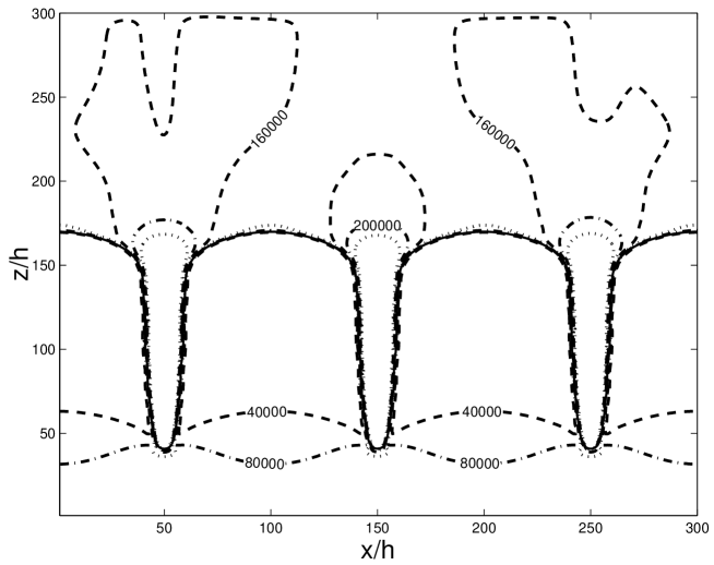
FIG. 6.: Stresses at $t=0.45$ (lowest curve in Fig. 4). Six contour values are displayed, the sequence of line patterns is dashed, dash-dotted, dotted with increasing value of $\sigma_{xx}$ and an increment of $4\times 10^{4}$ dynes/cm² between successive curves. To distinguish lines with the same pattern from each other, the values have been explicitly marked at those curves where there was enough room, e.g., for $\sigma_{xx}=4\times 10^{4}$ dynes/cm². The lower dash-dotted curve corresponds to the value of the applied external stress.

The next three figures show a simulation at a stress roughly 20% above the critical value. Our numerical box contains six wavelengths of the pattern initially. One of the grooves has however been made by 2% deeper than its neighbours. Contrary to the situation in Fig. 4, no prestress was applied, so a planar interface would move downward to a new equilibrium position. This kind of motion is superimposed on the shape-changing dynamics and serves nicely in separating the curves on the plot.

FIG. 7.: Dynamical evolution of a perturbed interface at $\sigma_{0}=1.16\,\sigma_{c}$ ($\sigma_{0}=3\times 10^{4}$ dynes/cm², $\epsilon=0.025$, $E=3.2\times 10^{8}$ dynes/cm²). MG model, no prestress. Time interval between curves 0.25; the final time is 2.5. After an initial phase of acceleration, the interface slows down and approaches a cycloid-like curve.

The temporal dynamics can be divided into several stages. At first, the sinusoidal pattern changes its shape in the way already discussed by Nozières [22]: the tips become flat, the grooves pointed. After some time, the interface becomes similar to a cycloid but with different depths of the grooves. Also, the dynamics almost comes to a halt. Below, we shall discuss the similarity with a cycloid in more detail (see Fig. 10). It holds up to $t=2.5$ approximately, which is the time of the lowest curve in Fig. 7. At this point the apparent periodicity of the pattern has doubled. (Of course, strictly speaking this periodicity has been broken from the outset by our making one groove a little deeper. But this was only to avoid its being broken by numerical noise in an uncontrolled manner, i.e., to introduce a well-defined perturbation.)

The groove that was ahead initially, wins the competition for the elastic field; the losing grooves fall back and even close again. This is shown in Fig. 8, displaying the temporal continuation of Fig. 7. In the initial structure of Fig. 8 (the solid line that is shallowest in the big grooves), the smaller grooves are deeper than in the final one (the dashed line which is deepest in the big grooves but shallowest in the small ones). At the end of the period of time depicted in Fig. 8, there are three clear survivors and three losers of the competition.

FIG. 8.: Continuation of the evolution from Fig. 7. Initial time $t=2.75$, time step $\Delta t=0.25$, final time $t=5.0$. The biggest groove is still accelerating, while the other even-numbered grooves have a roughly constant velocity and seem to decelerate towards $t=5.0$. Odd-numbered grooves retract. They are deepest at $t=2.75$ and have almost closed at $t=5.0$.

Finally, as shown in Fig. 9, only one groove survives. Its velocity is almost constant over a range of times. Eventually it slows down and grows sideways towards the end, which may have to do with the fact that it gets too close to the bottom of the numerical box (which is at $\zeta=-1$). Also gravity has a decisive decelerating effect here.

What we observe, then, is a coarsening process that seems to proceed via imperfect period doubling transitions. Because our system has only six grooves, we cannot explicitly see more than the first period doubling here. These transitions are local in the following sense. Not all grooves surviving the first period doubling get ahead of the others simultaneously. Rather what happens is that first the winning groove gets ahead of its nearest neighbours, screening each of them off the stress field on one side a little. This causes these neighbours to grow more slowly, making them screen off their next neighbours on the other side less. So these get ahead of their neighbour grooves, and so on. The perturbation made by one groove moves through the array in an alternating fashion. In an infinite system, one could imagine a series of “near” period doublings propagating through the array. These morphology changes are not exact period doubling transitions, because there is no restabilization of a structure with doubled periodicity. The system remains dynamic (but see the discussion on gravity below) which means that the foremost groove does not get slower than its competitors, which would be necessary for length adjustment.

FIG. 9.: Continuation of the evolution from Fig. 8. Initial time $t=5.25$, time step $\Delta t=0.25$, final time $t=8.0$. The winning groove has a constant velocity most of the time.

The first of these period doublings may be discussed analytically in some detail. Consider the shape of the interface close to the last time of Fig. 7. It can be modeled approximately by a curve that we would like to call a “double cycloid”. A parameter representation of this curve is given by

$$x = \xi-A\sin k\xi-B\sin 2k\xi$$ (51)

$$z = \phantom{\xi}-A\cos k\xi-B\cos 2k\xi$$ (52)

Figure 10 compares a double cycloid with the interface at $t=2$. The wavenumber $2k$ (= 9.425) is given by the basic periodicity of the initial interface (before it is perturbed), the amplitudes $A$ and $B$ have been fitted “by eye” and the double cycloid has been shifted using translational invariance in the $x$ direction. (Its position in the $z$ direction can also be adjusted, which corresponds to a particular choice of the initial chemical potential of the solid.)

FIG. 10.: Comparison of the interface at $t=2$ from Fig. 7 (dashed line) with a double cycloid (solid line).

Since we made only one of the grooves deeper than the others, the agreement of the groove minima is not quite perfect, as we can adjust only the depths of this groove and its nearest neighbours by an appropriate choice of the two constants $A$ and $B$. Had we taken an initial perturbation of periodicity length $2\pi/k$ instead of a local one in the simulation, a much better agreement would have been obtained. The purpose of this comparison, however, is not to claim that the interface shape goes precisely to a double cycloid but only to show that it may be well approximated by such a curve, which can be considered a cycloid (with amplitude $B$) modified by a small perturbation of twice its wavelength. In our fit shown in Fig. 10, we have $A\approx B/10$.

Our key observation is then that we can solve the sharp-interface elastic problem for a double cycloid exactly in an extension of the work of Gao et al. [24], using a conformal mapping technique. This solution is given in appendix C. In what follows, we will neglect the gravity term, a procedure that we justify later. The evaluation of the nondimensional velocity via Eq. (44) for the double cycloid yields, in the bottoms of the grooves [see appendix, Eq. (C41)]

$$\tilde{v}_{n}=-\frac{1}{2\left[1-k\left(A(-1)^{m}+2B\right)\right]^{2}}\left\{\left(1+2Bk+\frac{1+Bk}{1-Bk}Ak(-1)^{m}\right)^{2}-\alpha k\left[A(-1)^{m}+4B\right]\right\}\>,$$ (53)

where $\alpha=2k/q_{f}$ is the ratio of the actual wavenumber of the basic cycloid and the wavenumber of the fastest-growing mode. The formula with odd $m$ holds for the minima with depth $-2Bk+Ak$, that with even $m$ for those with depth $-2Bk-Ak$. A condition for the solution to hold is that there are no self-crossings of the curve, therefore we must require $Ak+2Bk<1$. Let us now assume that $A\ll B$, i.e. that the pattern actually is a slightly perturbed cycloid (where the perturbation has twice the basic wavelength $\pi/k$). Then the denominator in Eq. (53) in front of the braces goes to zero for even $m$ as $2Bk$ approaches the value 1. This is the finite-time singularity, already identified by Gao al. [24]. The velocity goes to $-\infty$, if the braces remain positive, which they do for small enough $\alpha$, i.e., when the wavelength is large enough. For small $A$, we can expand (53). This gives

$$\tilde{v}_{n} = -\frac{1}{2\left[1-k\left(A(-1)^{m}+2B\right)\right]^{2}}\Biggl{\{}(1-2Bk)^{2}+4(1-\alpha)Bk$$ (55)

$$\quad\quad\quad\quad\mbox{}+Ak(-1)^{m}\left[2\frac{(1+Bk)(1+2Bk)}{1-Bk}-\alpha\right]\Biggr{\}}\>,$$

a formula that shows that the marginal value of $\alpha$ is 1. Thus, for wavelengths larger than that corresponding to the fastest-growing mode ($\alpha\approx 1$), the velocity will diverge in the deepest minima, leading to cusps in the sharp-interface limit. We could leave the gravity term out of this consideration, because it never diverges for finite $\zeta$.

Now assuming we are at or slightly above the wavelength of the fastest-growing mode, we can see from (55) that for $(1-2Bk)^{2}<Ak$ the velocity is positive in the secondary minima corresponding to odd $m$ [32]. This means resolidification and closure of the corresponding grooves.

Suppose for a moment that $A=0$. Then the system with a sharp interface will evolve towards a cusped cycloid, i.e., $2Bk$ will increase towards 1. But this means that eventually a point will be reached where $1-2Bk$ is small enough that any perturbation will be larger than $(1-2Bk)^{2}$. In this case, our equations state that (for $1-\alpha\ll 1$) the tip perturbed in this way in the right direction (i.e., the perturbation must reduce the depth of the groove) will recede again, its velocity will become positive. A groove tip that is perturbed in the other direction will approach the cusp singularity even faster and reduce the speed of its neighbours. Of course, not all perturbations are periodic; what happens when only a local perturbation is applied, can be seen from the simulation.

What the analytic calculation shows, then, is that the first period-doubling bifurcation happens before the cusp singularity is reached, if the periodicity of the system is equal to the wavelength of the fastest-growing mode. Whereas the bifurcation to a set of alternatingly receding and advancing grooves may happen for any wavelength larger than this one, whether it happens before or after the predictable time of cusp formation will in general depend on the strength of the perturbations present in the system. In the simulation of Figs. 7-9, the periodicity of the unperturbed system is $\frac{2}{3}$, the wavelength of the fastest-growing mode is 0.5.

Ordinarily, the time when the finite-time singularity appears in the sharp-interface system will be too short for the losing grooves to have appreciably retracted. In our phase-field model, there are no finite-time singularities, so the evolution can continue. It is then highly plausible that further period doublings occur, even though we have no analytic model for these. But on general grounds, we expect screening of neighbouring grooves to become more effective as all grooves get deeper. Hence the process should repeat, even at wavelengths far from, but above, $\lambda_{f}$.

The difference between the cases of a wavelength close to that of the fastest-growing mode and one far above it is that in the former case, the first period doubling will happen before the time $t^{\ast}$, at which cusps form in the sharp-interface limit, whereas in the latter case, it will happen afterwards. This case is, in fact, realized in Fig. 4, where the wavelength of the fastest-growing mode is about one tenth of the periodicity length. From Fig. 6, we can infer that the translational symmetry with respect to the basic wavelength $\lambda=\frac{2}{3}$ has already been broken by numerical noise (the stress pattern does not show this periodicity in the upper half of the picture, this symmetry breaking will slowly propagate into the lower half where everything still appears periodic).

Another interesting conclusion from formula (53) is that for $\alpha>1$, i.e., for systems with small enough wavelength, stable steady states may be possible, because then surface tension may succeed in overwhelming the effects of stress. For $\alpha>1$ and $A=0$, the formula predicts that a cycloid becomes stationary in its minima before the appearance of cusps. We hope to report on this aspect in the future.

Finally, let us have a look at a system with a random initial condition. Figure 11 shows the evolution starting from an interface resulting from uniformly random perturbations of a planar front. We see that first some 10 waves develop, which is already a coarsened structure, as the wavenumber of the fastest-growing linear mode would correspond to about 24 waves fitting into the system. However, the initial amplitude is too small for this wavelength to become clearly visible. Some time later, there are much fewer features and eventually, only two grooves remain.

FIG. 11.: Evolution of a random interface. $\sigma_{0}=3.5\times 10^{4}$ dynes/cm², $\epsilon=0.05$. Periodic boundary conditions, i.e., MG model. $0\leq t\leq 11.6$, $\Delta t=0.4$.

Whether one of the two will die off in the end is not clear, since this is a simulation with gravity. Hence the largest groove is bound to stop at some time, because the stress and curvature terms remain constant once all other grooves are sufficiently small, but the gravity term continues to increase. If the second-largest groove still has a positive velocity when the first stops, it will not reverse its growth direction, but only grow to a point where its velocity becomes zero.

An example, where the final state actually consists of two grooves, is shown in Fig. 12. Here the applied stress is smaller than in Fig. 11, so the pattern actually does come to a halt within the numerical box, after a long time ($t\approx 60$). Note that during most of the period where two grooves are dominant, one of them is ahead. Once it stops, the second approaches and in the end it has the same length as the first, to numerical accuracy. In the case of two periodically repeated grooves, this is to be expected for symmetry reasons. With three or more grooves, it is also conceivable that not all of them are the same length in the steady state.

FIG. 12.: Evolution of a random interface with periodic boundary conditions. $\sigma_{0}=2.8\times 10^{4}$ dynes/cm², $\epsilon=0.035$, $0<t\leq 80.0$, $\Delta t=0.8$. The final interface has only two grooves and no further substructure. It is symmetric with respect to two symmetry axes at the two possible central positions between the two grooves.

We think that in the absence of gravity, the situation in this strongly nonlinear region is very similar to the evolution of a Saffmann-Taylor finger in a Laplacian field. The Lamé equations determining the displacement field are scale invariant just as the Laplace equation (and in fact, Eq. (44) is scale invariant for $\ell_{2}=\infty$). Once a strongly nonlinear state has been reached, none of the length scales discussed in section II can play a role anymore, since they only govern the local behavior of the growth pattern. The long-range elastic field will determine the factor $\sigma_{tt}-\sigma_{nn}$ of the destabilizing term in (44) and this factor will be the larger, the fewer competitors of a groove have grown to the same depth. This will lead to smaller grooves not growing anymore. This situation bears strong similarities to the growth of thermal cracks described in [33]. The main difference is that there a loser in the competition will simply stop growing. In our case, it will even shrink again, for the crystal can not only melt but also freeze again, and whether it will do so is simply determined by the chemical potential difference (1).

An analogous behavior is found in the side branching activity of a dendrite in the region about 20 to 50 tip radii behind the tip [34, 35]. There coarsening is observed, too, which also proceeds via imperfect period doubling. If this dynamics can be described in terms of a series of nonequilibrium phase transitions at all, these would have to be considered first-order transitions because of the discussed locality aspect. There is no diverging length scale in a single transition.

We expect that the dynamics of large systems can be described by scaling laws similar to those given previously for the growth of needles in a Laplacian field [36]. The fact that “needles” can shrink again in the elastic problem should modify the long-time behavior of the needle density, which must pass through a maximum and then go to zero as a function of time, for any needle length.

To some extent, this expectation is supported by the coarsening scenario described in [17] in which extended systems without gravity are studied using random initial conditions. They measured the Fourier transform of the height-height correlation function $S(q,t)$ and observed dynamical scaling. For early times, they observed a strong similarity between this behavior and early-stage soinodal decomposition in long-range systems. For later times, when the linear theory no longer describes the data, coarsening is evident: The location of the peak $q_{\rm max}$ of $S(q,t)$ moves to smaller wavenumbers, as the peak height increases and sharpens. The peak height follows $S(q_{\rm max},t)\sim t^{\alpha+1}$, where $\alpha\approx 2$, while the peak width sharpens with time as $w\sim t^{-\gamma}$, where $\gamma\approx 0.5$. The former dependence is due to the total interface length increasing linearly with time for any unstable wavenumber. The latter dependence is due to competitive ordering between different wavenumbers, analogous to phase ordering. Within the accuracy of their study, they find that the structure factor shows scale invariance: $S(q,t)/S(q_{\rm max},t)=S^{*}(q^{*})$, where the scaled wave number $q^{*}=(q-q_{\rm max})/w$. Fitting to $S^{*}\sim(q^{*})^{\delta}$ and $S^{*}\sim(1/q^{*})^{\psi}$, for small and large $q^{*}$ respectively, gives $\delta\sim 1-2$, and $\psi\sim 5-6$.

It is however difficult to assess to which time regimes these results correspond when compared with the present simulations, because the freedom to rescale parameters has been used extensively in [17]. Since the vanishing of grooves does not seem to be a dominant mechanism of coarsening in their simulations, it is likely that the time windows considered in [17] and here have little overlap and that the stage of needle-like growth of the grooves is never reached in [17]. Of course, the concept of short and long times is ambiguous in the absence of gravity due to the scale invariance of (44) for $\ell_{2}=\infty$. However, one can compare the depths of grooves with their lateral distances to decide whether growth is best described as competition of wavenumbers (a Fourier space concept) or as competition of needles (a real-space concept). In this context, it is also important to realize that the validity of the simulations in [17] is restricted to small values of $\mu/K$ with the parameter $\eta_{0}$ (see app. B) being $O(1)$, hence these simulations are quantitative only for external stresses $\sigma_{0}=O(\mu)$. For these stresses, the state describable as a forest of needles is only obtained after a long time [of order $(K/\mu)^{4}$]. Therefore, the scaling exponents obtained in [17] might not be relevant to the scenario discussed here, which makes an analytic treatment along the lines of [36] even more desirable, because it could provide these exponents.

In an infinite system what we have depicted here is probably just the continuation of the coarsening scenario described in [17].

It should also be pointed out that for sufficiently wide systems, i.e., in particular for infinite ones, this dynamics may be an intermediate state only. Once a groove becomes sufficiently long, stresses along its side may become large enough to provoke a Grinfeld instability of the “side walls” of this crack-like structure, as has been shown by Brener and Marchenko [38]. Whether or not this happens, depends on how efficiently the stresses are relaxed along the grooves, on the speed of the grooves, on the perturbation amplitude, etc. This secondary instability might completely change the scaling behavior, possibly leading to tip splitting of the grooves and tree-like structures. So far, we have not seen anything of this kind in our simulations.

In a system of finite lateral extent (or periodicity) we think coarsening will in the absence of gravity generally lead to the disappearance of all grooves except one which will grow at constant velocity. If gravity is present, several grooves can survive and in a sufficiently deep system they will stop once they reach a depth where the gravity term compensates the stress one.

IV Conclusions

In this article, we have constructed a class of phase-field models from a free-energy functional including the elastic energy density. A salient feature of the model is that the liquid is treated as a shear-free solid, which is to be contrasted with phase-field models taking into account hydrodynamic effects in solidification, where the solid is usually treated as a liquid of infinite viscosity [37]. Our approach implies the artificial introduction of coherence conditions at the interface which is however counterbalanced by the fact that the only relevant elastic variable in the liquid is $\nabla{\bf u}$. A whole class of models is obtained instead of a single one as a consequence of the freedom of choice for the state of reference used in measuring displacements. We compared the two most natural choices and found them to yield slightly different numerical results despite their asymptotic equivalence.

Investigating a large number of laterally small and extended systems, we believe to be able now to describe the generic dynamic behavior. For systems smaller than the wavelength of the fastest-growing mode of linear stability theory but larger than that of the marginal mode (where surface tension stabilizes the planar interface), stable steady-state strucures are possible even in the sharp-interface limit. This is similar to the findings by Spencer and Meiron [23] for the case of transport via surface diffusion, even though we think the whole picture is more complex than what they described [39]. Here, we did not show detailed results on small systems but focused on extended systems.

The case without gravity is particularly simple, as the equation of motion can then be made parameter free [Eq. (44) without the last term]. Initially, an interface may grow periodically but as soon as perturbations break the periodicity, coarsening will proceed via approximate period doubling transitions. Supposing randomized perturbations, the interface will, after a sufficient lapse of time, not look much different from one started with random initial conditions (compare Figs. 9 and 11). If the system is of finite lateral extent (but infinitely deep), only a single groove will survive growing at constant velocity, determined by the final constant stress and constant surface tension terms near its tip. The final velocity will scale with the system width $L$ and the radius of curvature $\epsilon$ as $v_{n}\sim L/\epsilon$. All the other grooves will eventually retract, i.e., they will not even survive keeping a finite depth, which is different from the behavior of cracks [33]. For wide systems, stresses near the groove tips may become large enough to trigger a secondary instability [38] which would considerably modify the system behavior and allow the appearance of complex crack morphologies. It is however possible that this will arise only in the case of finite perturbations, as grooves may grow too fast in this situation for the instability to develop before it is “advected” (relative to the groove tip) into a region of very small stresses along the groove. If the system is laterally infinite, the system state will first follow dynamical scaling as studied in [17] and should then cross over to the scaling dynamics described here with the number of grooves continually decreasing according to a power law, possibly with logarithmic corrections. Alternatively, the coarsening scenarios observed in [17] and in this article might be governed by the same scaling laws, with their difference being only apparent. The emphasis of [17] was on the scaling laws governing coarsening, that of the present study is on the mechanism of coarsening. Obviously, this situation calls for large-scale simulations in order to determine the scaling exponents in cases where the mechanism presented here is definitely at work already.

If the mentioned secondary instability [38] becomes important, the identified state of competing grooves will be only of intermediate nature. Of course, all our considerations hold only as long as linear elasticity remains valid in the bulk, nonlinear elastic effects may alter the scenario.

With gravity included (which was not considered in [17]), there are some modifications. First, it is now possible for a planar interface to be stable (apart from a vertical translation). Once the threshold of the instability has been exceeded, the behavior will be similar to the case without gravity. However, we predict that it is possible for several grooves to survive in a finite system and that they will eventually stop growing, because the stress does not increase beyond a certain magnitude due to the lateral system width, whereas the gravity term increases as long as a groove gets deeper. That several grooves may survive has to do with the fact that now we have length scales in Eq. (44). More simple-mindedly we can immediately see that once the biggest groove stops, the second-largest will not retract, if it still has a downward velocity at that moment. Once the second stops, we can repeat the argument for the third, and so on. The final state will consist of a number of grooves, probably of different lengths and disordered. (For large-width systems, the aforementioned secondary instability may again complicate the picture.) In laterally infinite systems, it seems likely that a scaling state will prevail, possibly with a modified scaling exponent. Because now both stresses at the tips of the largest grooves and the gravity terms continue to grow, but they will both grow linearly with the length of the grooves. If initially the stress was large enough to overcompensate the gravity term, it will presumably stay like that. It is, however, not excluded that starting from specific initial conditions a system can be stabilized by gravity in the end.

Acknowledgments

This work was supported by the German Research Society (Deutsche Forschungsgemeinschaft) under grant Ka 672/4-2, which is gratefully acknowledged. Moreover, we acknowledge a PROCOPE grant for travel exchanges by the DAAD (German academic exchange service), grant no. 9619897, and the A.P.A.P.E. (corresponding French organisation), grant no. 97176, as well as financial support by the TMR network “Pattern formation, noise and spatio-temporal chaos in complex systems”.

A Derivation of the sharp-interface limit

In deriving the sharp-interface limit, we will restrict ourselves to the two-dimensional case as we did in discussing the sharp-interface equations (where we used only two stress components and only one curvature). The generalization to three dimensions is, however, straightforward. We may use (39) and (42) as outer equations, to be used in the regions where the gradient of the phase field is small. For convenience, we set $z_{0}=0$.

To obtain the inner equations, we transform to a local system of (orthogonal) curvilinear coordinates comoving with the interface, with one coordinate axis parallel to $\nabla\phi$; the corresponding coordinate will be called $r$, while the second will be conveniently expressed by the arclength $s$ along the interface [40]. We introduce a stretched variable setting $r=\tilde{\epsilon}\rho$. It is then easy to see that a distinguished limit of (39), leading to a nontrivial inner equation that allows to satisfy the boundary conditions, is obtained by setting $\tilde{\epsilon}=\epsilon$. In saying this, we have assumed that the stresses and strains behave properly under rescaling, i.e., do not diverge. Designating by capital letters the values of the fields in the inner domain (where the gradient of the phase field is large), we then have the inner equations

$$-\frac{v}{\epsilon}\>{\partial_{\rho}}\Phi = \frac{\gamma}{{\tilde{k}}}\>\Biggl{\{}\frac{1}{\epsilon^{2}}{\partial_{\rho}^{2}}\Phi+\frac{\kappa}{\epsilon}\>{\partial_{\rho}}\Phi+{\partial_{s}^{2}}\Phi-\frac{1}{\epsilon^{2}}\Biggl{[}2g^{\prime}(\Phi)$$ (A2)

$$\mbox{}+\frac{\epsilon}{3\gamma}h^{\prime}(\Phi)\left(\mu\,U_{ij}U_{ij}+\frac{\lambda-\tilde{\lambda}}{2}U_{ii}^{2}+\Delta p\,U_{ii}+\Delta W+\Delta\rho gz\right)\Biggr{]}\Biggr{\}}\>,$$

$$0 = \frac{1}{\epsilon}\>{\partial_{\rho}}\tilde{\Sigma}_{\rho\rho}+{\partial_{s}}\tilde{\Sigma}_{\rho s}+\kappa\left(\tilde{\Sigma}_{\rho\rho}-\tilde{\Sigma}_{ss}\right)\>,$$ (A3)

$$0 = \frac{1}{\epsilon}\>{\partial_{\rho}}\tilde{\Sigma}_{s\rho}+{\partial_{s}}\tilde{\Sigma}_{ss}+\kappa\left(\tilde{\Sigma}_{\rho s}+\tilde{\Sigma}_{s\rho}\right)\>,$$ (A4)

where

$$\tilde{\Sigma}_{\alpha\beta}=h(\Phi)\Sigma_{\alpha\beta}-(1-h(\Phi))P\delta_{\alpha\beta}$$ (A5)

is the generalized stress tensor of the two-phase system. In order to obtain (A2–A4), we have used

$$\nabla = \frac{1}{\epsilon}\>{\bf n}\>{\partial_{\rho}}+{\bf t}\>{\partial_{s}}\>,$$ (A6)

$$\nabla^{2} = \frac{1}{\epsilon^{2}}\>{\partial_{\rho}^{2}}+\frac{\kappa}{\epsilon}\>{\partial_{\rho}}+{\partial_{s}^{2}}\>.$$ (A7)

Derivatives such as $\partial_{x}u_{x}$ can then be expressed in invariant form as ${\bf e}_{x}({\bf e}_{x}\nabla){\bf u}$, which leads to the following relations for the strain tensor components in the new coordinates:

$$U_{\rho\rho} = \frac{1}{\epsilon}\>{\partial_{\rho}}U_{\rho}\>,$$ (A8)

$$U_{ss} = {\partial_{s}}U_{s}+\kappa U_{\rho}\>,$$ (A9)

$$U_{\rho s} = U_{s\rho}\mbox{}=\mbox{}\frac{1}{2}\left({\partial_{s}}U_{\rho}+\frac{1}{\epsilon}\>{\partial_{\rho}}U_{s}-\kappa U_{s}\right)\>.$$ (A10)

The next step consists in solving the outer and inner equations via an asymptotic analysis that leads to a globally valid approximation for small interface thickness $\epsilon$ which approaches the sharp-interface equations as $\epsilon\to 0^{+}$. To this end we expand both outer and inner fields in powers of $\epsilon$:

$$\phi(x,z,t) = \phi_{0}(x,z,t)+\epsilon\phi_{1}(x,z,t)+...\>,$$ (A11)

$$u_{ij}(x,z,t) = u_{ij}^{(0)}(x,z,t)+\epsilon u_{ij}^{(1)}(x,z,t)+...\>,$$ (A12)

and

$$\phi(x,z,t) = \Phi(\rho,s,t)=\Phi_{0}(\rho,s,t)+\epsilon\Phi_{1}(\rho,s,t)+...\>,$$ (A13)

$$u_{ij}(x,z,t) = U_{ij}(\rho,s,t)=U_{ij}^{(0)}(\rho,s,t)+\epsilon U_{ij}^{(1)}(\rho,s,t)+...\>,$$ (A14)

where, due to the transformation properties of tensors, we can think of the subscripts $i$, $j$ as running either over the values ($x$,$z$) or ($r$,$s$) and ($\rho$,$s$), respectively. Our basic field equations are, however, equations not for the strains but for the displacement fields. Thus, the expansion of the $U_{ij}(\rho,s,t)$ induces one for the displacement components:

$$u_{r} = U_{\rho}(\rho,s,t)=U_{\rho}^{(0)}(\rho,s,t)+\epsilon U_{\rho}^{(1)}(\rho,s,t)+...\>,$$ (A15)

$$u_{s} = U_{s}(\rho,s,t)=U_{s}^{(0)}(\rho,s,t)+\epsilon U_{s}^{(1)}(\rho,s,t)+...\>.$$ (A16)

Now the physical requirement that both $u_{r}$ and $u_{s}$ remain finite in the limit $\epsilon\to 0^{+}$ allows us to conclude from (A8) and (A10) that neither $U_{\rho}^{(0)}$ nor $U_{s}^{(0)}$ can depend on $\rho$, hence

$$U_{\rho}^{(0)} = U_{\rho}^{(0)}(s,t)\>,$$ (A17)

$$U_{s}^{(0)} = U_{s}^{(0)}(s,t)\>.$$ (A18)

Furthermore, we have matching conditions for $1\ll\rho\ll\epsilon^{-1}$ that can be obtained from the inner and outer expansions by equating equal powers of $\epsilon$ (and taking into account that the variable $r$ is itself $\epsilon$ dependent):

$$\Phi_{0}(\rho,s,t) \sim \phi_{0}(r,s,t)|_{r=\pm 0}\>,\quad\quad\rho\to\pm\infty\>,$$ (A19)

$$\Phi_{1}(\rho,s,t) \sim [\phi_{1}(r,s,t)+\rho\>\partial_{r}\phi_{0}(r,s,t)]|_{r=\pm 0}\>,\quad\quad\rho\to\pm\infty\>,$$ (A20)

$$U_{\alpha\beta}^{(0)}(\rho,s,t) \sim u_{\alpha\beta}^{(0)}(r,s,t)|_{r=\pm 0}\>,\quad\quad\rho\to\pm\infty\>,$$ (A21)

where we use the $\sim$ symbol in the sense of asymptotic equality, i.e., $f(x)\sim g(x)$, $x\to x_{0}$ is equivalent to $\lim_{x\to x_{0}}f(x)/g(x)=1$, and for two series in $x-x_{0}$ we require this relation for each corresponding pair of terms.

The relations induced by (A21) for the displacements are more complicated. We just give two examples. Because each derivative with respect to $r$ comes with a factor $1/\epsilon$ when transformed into a derivative w.r.t. $\rho$, we have $U_{\rho\rho}^{(0)}=\partial_{\rho}U_{\rho}^{(1)}$ and hence

$$\lim_{\rho\to\pm\infty}\partial_{\rho}U_{\rho}^{(1)}(\rho,s,t)=\partial_{r}u_{r}^{(0)}(r,s,t)|_{r=\pm 0}\>.$$ (A22)

Our second example is even more instructive. We write

$$\lim_{\rho\to\pm\infty}U_{ss}^{(0)}(\rho,s,t) = \lim_{\rho\to\pm\infty}\left(\partial_{s}U_{s}^{(0)}(s,t)+\kappa U_{\rho}^{(0)}(s,t)\right)$$ (A23)

$$= \partial_{s}U_{s}^{(0)}(s,t)+\kappa U_{\rho}^{(0)}(s,t)$$ (A24)

$$= [\partial_{s}u_{s}^{(0)}(r,s,t)+\kappa u_{\rho}^{(0)}(r,s,t)]|_{r=\pm 0}\>,$$ (A25)

which shows that the linear combination $u_{s}^{(0)}+\kappa u_{\rho}^{(0)}$ must be continuous across the interface.

Finally, we need the expansions of all functions of $\phi$ in powers of $\epsilon$, e.g.:

$$h(\phi)=h(\phi_{0})+\epsilon h^{\prime}(\phi_{0})\phi_{1}+\epsilon^{2}\left(h^{\prime}(\phi_{0})\phi_{2}+\frac{1}{2}h^{\prime\prime}(\phi_{0})\phi_{1}^{2}\right)+...\>,$$ (A26)

and we will use the obvious abbreviations $h_{0}$, $h_{0}^{\prime}$, etc., for functions of $\phi_{0}$. Let us note a few useful relations in passing:

$$h^{\prime}(\phi) = 6\phi(1-\phi)\>,$$ (A27)

$$g(\phi) = \phi^{2}(1-\phi)^{2}=\left(\frac{1}{6}h^{\prime}(\phi)\right)^{2}\>,$$ (A28)

$$g^{\prime}(\phi) = 2\phi(1-\phi)(1-2\phi)=\frac{1}{18}h^{\prime}(\phi)h^{\prime\prime}(\phi)\>,$$ (A29)

We have now collected all the prerequisites to perform the asymptotic analysis providing the sharp-interface limit.

First, we note that the outer solution to lowest order [order $\epsilon^{-2}$ of (39)] is simply given by $g^{\prime}(\phi_{0})=0$, which yields the solutions $\phi_{0}=0$, $\phi_{0}=1$, and $\phi_{0}=\frac{1}{2}$ [see (A29)]. The last of these is unstable and also not compatible with the boundary conditions in typical numerical setups. We assume $\phi_{0}=0$ for $r>0$, corresponding to the liquid phase, and $\phi_{0}=1$ for $r<0$, corresponding to the solid phase. Equation (A27) tells us that $h^{\prime}(\phi_{0})=0$, and hence these solutions are valid at all orders of $\epsilon$. Using $h(\phi_{0})=0$ in the liquid and $h(\phi_{0})=1$ in the solid, we immediately see that (42) turns into the mechanical equilibrium condition for the liquid and solid, respectively:

$$\partial_{i}p = 0\quad\quad\mbox{(liquid)}\>,$$ (A30)

$$\partial_{j}\sigma_{ij} = 0\quad\quad\mbox{(solid)}\>.$$ (A31)

This is again true at all orders of $\epsilon$, and we can write the zeroth-order piece of the result in the form:

$$p^{(0)} = p_{0\ell}-{\tilde{\lambda}}u_{kk}^{(0)}=p_{0}={\rm const.}\>,$$ (A32)

$$\sigma_{ij}^{(0)} = -p_{0s}\delta_{ij}+2\mu u_{ij}^{(0)}+\lambda u_{kk}^{(0)}\delta_{ij}\>.$$ (A33)

Later, we will look at two reference states in particular. One is the “natural” choice $p_{0s}=p_{0\ell}$, i.e., the unstrained state is hydrostatic and corresponds to the same pressure in the liquid and in the solid. If moreover, this pressure is chosen equal to the equilibrium pressure $p_{0}$, then we have $u_{kk}^{(0)}\equiv 0$ in the liquid at equilibrium. The second choice corresponds to assuming a finite difference $\Delta p=p_{0\ell}-p_{0s}$ while keeping $p_{0\ell}=p_{0}$. This means that zero strain corresponds to a prestressed solid, with a stress tensor $\sigma_{ij}=-p_{0}\delta_{ij}+\Delta p\,\delta_{ij}$, i.e., the deviation from equilibrium is the isotropic tensor $\Delta p\,\delta_{ij}$. Both approaches can be exploited numerically.

We now consider the inner solution. The lowest order of (A2) gives

$$\partial_{\rho}^{2}\Phi_{0}-2g^{\prime}(\Phi_{0})=0\>.$$ (A34)

This equation can be solved by standard methods. Multiplying by $\partial_{\rho}\Phi_{0}$, we immediately obtain a first integral, written down here for further reference,

$$\partial_{\rho}\Phi_{0}=-2\Phi_{0}(1-\Phi_{0})=-\frac{1}{3}h_{0}^{\prime}\>,$$ (A35)

which is solved by $\Phi_{0}=\frac{1}{2}(1-\tanh\rho)$, and this solution satisfies the matching conditions (A19).

From the strain equations (A3), (A4) we obtain to lowest order

$$\partial_{\rho}\tilde{\Sigma}^{(0)}_{\rho\rho} = 0\>,$$ (A36)

$$\partial_{\rho}\tilde{\Sigma}^{(0)}_{s\rho} = 0\>,$$ (A37)

which on integration from $\rho=-\infty$ to $\rho=\infty$ together with the matching conditions (A21) yields

$$\sigma^{(0)}_{rr}|_{r=0^{-}} = \tilde{\Sigma}^{(0)}_{\rho\rho}(-\infty)=\tilde{\Sigma}^{(0)}_{\rho\rho}(\infty)=-P=-p_{0}\>,$$ (A38)

$$\sigma^{(0)}_{sr}|_{r=0^{-}} = \tilde{\Sigma}^{(0)}_{s\rho}(-\infty)=\tilde{\Sigma}^{(0)}_{s\rho}(\infty)=0\>.$$ (A39)

The limiting values of $\tilde{\Sigma}^{(0)}_{\rho\rho}$ and $\tilde{\Sigma}^{(0)}_{s\rho}$ can be gathered from (A5). Obviously, these two equations constitute the condition of mechanical equilibrium at the interface, as $\sigma^{(0)}_{rr}$ and $\sigma^{(0)}_{sr}$ are the normal and shear components of the stress tensor of the outer solution there.

However, the strain equations provide more information than just mechanical equilibrium on the outer scale. We write (A36) explicitly in terms of the strains and integrate indefinitely with respect to $\rho$, which yields

$$h_{0}\left[(2\mu+\lambda-{\tilde{\lambda}})U_{\rho\rho}^{(0)}+(\lambda-{\tilde{\lambda}})U_{ss}^{(0)}+\Delta p\right]+{\tilde{\lambda}}(U_{\rho\rho}^{(0)}+U_{ss}^{(0)})=f(s,t)\>,$$ (A40)

where $f(s,t)$ is a function of integration, to be determined from the matching conditions. This is straightforward and yields $f(s,t)=p_{0\ell}-p_{0}$. Moreover, we know that the only spatial dependence of $U_{ss}^{(0)}$ is that on $s$ [see (A25) and (A18)], which suggests to solve for $U_{\rho\rho}^{(0)}$ in terms of $U_{ss}^{(0)}$. The result is

$$U_{\rho\rho}^{(0)} = \frac{-1}{(2\mu+\lambda-{\tilde{\lambda}})h_{0}+{\tilde{\lambda}}}\biggl{\{}\Delta p\>h_{0}+p_{0}-p_{0\ell}+[{\tilde{\lambda}}+(\lambda-{\tilde{\lambda}})h_{0}]U_{ss}^{(0)}\biggr{\}}\>.$$ (A41)

The advantage of this equation is that it provides us with the full $\rho$ dependence of $U_{\rho\rho}^{(0)}$, allowing the explicit evaluation of integrals on $\rho$ containing the strains. An analogous procedure for the second strain equation determines $U_{s\rho}^{(0)}$ to be equal to zero.

Now we proceed to the next-order equation for $\Phi$. Written out explicitly, it reads

$$-v\partial_{\rho}\Phi_{0} = \frac{\gamma}{{\tilde{k}}}\biggl{\{}\partial_{\rho}^{2}\Phi_{1}+\kappa\partial_{\rho}\Phi_{0}-2g^{\prime\prime}_{0}\Phi_{1}$$ (A44)

$$\mbox{}-\frac{h^{\prime}_{0}}{3\gamma}\Bigl{(}\mu\bigl{[}{U_{\rho\rho}^{(0)}}^{2}+{U_{ss}^{(0)}}^{2}\bigr{]}+\frac{\lambda-{\tilde{\lambda}}}{2}\bigl{(}U_{\rho\rho}^{(0)}+U_{ss}^{(0)}\bigr{)}^{2}$$

$$\mbox{}+\Delta p\bigl{(}U_{\rho\rho}^{(0)}+U_{ss}^{(0)}\bigr{)}+\Delta W+\Delta\rho gz(s)\Bigr{)}\biggr{\}}$$

where we have used $U_{s\rho}^{(0)}=0$. With the help of (A27) and (A35), we can arrange this as

$$L\Phi_{1} = \frac{h^{\prime}_{0}}{3\gamma}\biggl{\{}{\tilde{k}}v+\gamma\kappa+\mu\bigl{[}{U_{\rho\rho}^{(0)}}^{2}+{U_{ss}^{(0)}}^{2}\bigr{]}+\frac{\lambda-{\tilde{\lambda}}}{2}\bigl{(}U_{\rho\rho}^{(0)}+U_{ss}^{(0)}\bigr{)}^{2}$$ (A46)

$$\mbox{}+\Delta p\bigl{(}U_{\rho\rho}^{(0)}+U_{ss}^{(0)}\bigr{)}+\Delta W+\Delta\rho gz(s)\biggr{\}}\>,$$

with $L\equiv\partial_{\rho}^{2}-2g^{\prime\prime}_{0}$ being a self-adjoint linear operator. The solvability condition for this inhomogeneous linear equation is that the right-hand side be orthogonal to the left-sided null eigenspace of $L$. Since $L$ is hermitean, we know that the translational mode $\partial_{\rho}\Phi_{0}$ is an appropriate eigenvector:

$$\partial_{\rho}\Phi_{0}L=L\partial_{\rho}\Phi_{0}=0\>.$$ (A47)

Multiplying (A46) by $3\gamma\partial_{\rho}\Phi_{0}$ from the left and integrating on $\rho$, we find

$$0 = \int_{-\infty}^{\infty}\,d\rho\>\biggl{\{}{\tilde{k}}v+\gamma\kappa+\mu\bigl{[}{U_{\rho\rho}^{(0)}}^{2}+{U_{ss}^{(0)}}^{2}\bigr{]}+\frac{\lambda-{\tilde{\lambda}}}{2}\bigl{(}U_{\rho\rho}^{(0)}+U_{ss}^{(0)}\bigr{)}^{2}$$ (A49)

$$\mbox{}+\Delta p\bigl{(}U_{\rho\rho}^{(0)}+U_{ss}^{(0)}\bigr{)}+\Delta W+\Delta\rho gz(s)\biggr{\}}h^{\prime}_{0}\partial_{\rho}\Phi_{0}\>.$$

Now we can exploit (A41), telling us that the $\rho$ dependence of the braces in (A49) is fully contained in their dependence on $h_{0}$. All the integrals can be done analytically, using

$$I\equiv-\int_{-\infty}^{\infty}\,d\rho\>f(h_{0})h^{\prime}_{0}\partial_{\rho}\Phi_{0}=-\int_{1}^{0}\,d\Phi_{0}\>f(h(\Phi_{0}))h^{\prime}(\Phi_{0})=\int_{0}^{1}\,dh\>f(h)\>.$$ (A50)

Integrals that appear in (A49) are

$$I_{1} = -\int_{-\infty}^{\infty}\,d\rho\>h^{\prime}_{0}\partial_{\rho}\Phi_{0}=1\>,$$ (A51)

$$I_{2} = -\int_{-\infty}^{\infty}\,d\rho\>U_{\rho\rho}^{(0)}h^{\prime}_{0}\partial_{\rho}\Phi_{0}\>,$$ (A52)

$$I_{3} = -\int_{-\infty}^{\infty}\,d\rho\>{U_{\rho\rho}^{(0)}}^{2}h^{\prime}_{0}\partial_{\rho}\Phi_{0}\>.$$ (A53)

The evaluation of the latter two integrals is as straightforward as that of the first, although a little more tedious. We just give the final result for the solvability condition, taking $p_{0\ell}=p_{0}$ for simplicity:

$$-{\tilde{k}}v=\gamma\kappa+\Delta\rho gz+\frac{\mu}{2(\mu+\lambda)(2\mu+\lambda)}\left[2(\mu+\lambda)U_{ss}^{(0)}+\Delta p\right]^{2}-\frac{2\mu+\lambda}{8\mu(\mu+\lambda)}\sigma_{00}^{2}\>,$$ (A54)

At this point, we may specify our choice of reference state for the solid. First, let us assume that the unstrained state corresponds to a state of equal hydrodynamic pressure in the two phases, i.e. $p_{0s}=p_{0\ell}$, or $\Delta p=0$. This is the KM choice. Then taking the limit $\rho\to-\infty$ of (A41) we get ($U_{ss}^{(0)}=u_{ss}^{(0)}$)

$$u_{rr}^{(0)}=\frac{-\lambda u_{ss}^{(0)}}{2\mu+\lambda}\>,$$ (A55)

implying $\sigma_{ss}^{(0)}-\sigma_{rr}^{(0)}=2\mu(u_{ss}^{(0)}-u_{rr}^{(0)})=4\mu(\mu+\lambda)u_{ss}^{(0)}/(2\mu+\lambda)$, from which we obtain

$$u_{ss}^{(0)}=\frac{2\mu+\lambda}{4\mu(\mu+\lambda)}(\sigma_{tt}^{(0)}-\sigma_{nn}^{(0)})\>,$$ (A56)

where we have now switched to the conventional notation for the principal components of the stress tensor in the normal and tangential directions ($\sigma_{rr}=\sigma_{nn}$, $\sigma_{ss}=\sigma_{tt}$). Finally, expressing the Lamé constants by Young’s modulus and the Poisson ratio, we arrive at

$$v=-\frac{1}{{\tilde{k}}}\biggl{\{}\frac{1-\nu^{2}}{2E}\left[(\sigma_{tt}^{(0)}-\sigma_{nn}^{(0)})^{2}-\sigma_{00}^{2}\right]+\gamma\kappa+\Delta\rho gz\biggr{\}}\>,$$ (A57)

which is the desired sharp-interface limit. [In eqs. (1, 2), $\sigma_{00}=0$.]

A remark is in order here. The phase-field equations imply the continuity of $u_{ss}^{(0)}$ across the interface. As this quantity is obviously nonzero whenever the solid is strained, this means that we will not have $u_{ss}^{(0)}=0$ in the liquid. However, we will still have $u_{ss}^{(0)}+u_{rr}^{(0)}=0$, i.e., the divergence of the displacement vector vanishes in the liquid. But this is all that matters, because it is only this quantity that enters the description of the liquid.

The reason for $u_{ss}^{(0)}\neq 0$ in the liquid is that the phase-field description imposes coherence of the strain across the interface, which ultimately goes back to our viewing the liquid as a (shear-free, but nonetheless) solid. For a true liquid in contact with a solid there is no such coherence condition as it is free to slip on the solid surface. Therefore, it could always keep its strain tensor isotropic (if such a notion made much sense at all for a liquid). The reason why we can nevertheless model the liquid as a solid is the additional degree of freedom that arises in the description of a liquid by having two fields $u_{x}$ and $u_{z}$ at our disposal even though only their combination $\nabla{\bf u}$ enters the free-energy expression. Therefore, we can compensate, so to speak, for imposing (nonphysical) coherence by allowing (equally nonphysical) anisotropic strain in the liquid.

At this point we may also note that if we were to model the elastic properties of two real solids by the current phase-field approach, we would necessarily impose coherence at the interface. The treatment of noncoherent solid-solid interfaces via phase fields would require some rethinking of the method.

Concerning computational purposes, one disadvantage of the chosen reference state is that it is not very well-suited for the use of periodic boundary conditions, meaning periodically varying stresses and strains. The field equations are set up in terms of the displacements which acquire linearly increasing or decreasing components in directions where the strain has a nonzero average. This observation motivates the consideration of a different reference state in the solid, in which the average strain due to the external stress is subtracted. This is the MG choice (see App. B). If we impose a constant stress $\sigma_{0}$ in the $x$ direction, the stress tensor in the solid is $\sigma_{ij}=-p_{0}\delta_{ij}+\sigma_{0}\delta_{i1}\delta_{1j}$ and requiring $u_{xx}=0$, we find that this is achieved by setting

$$\Delta p=\frac{2\mu+\lambda}{2\mu}\sigma_{0}\>.$$ (A58)

The corresponding homogeneous strain tensor is given by $u_{xx}=0$, $u_{xz}=0$, and $u_{zz}=-\Delta p/(2\mu+\lambda)$. We then obtain taking the limit $\rho\to-\infty$ of (A41)

$$u_{rr}^{(0)}=\frac{-\Delta p-\lambda u_{ss}^{(0)}}{2\mu+\lambda}\>.$$ (A59)

This can be used to express

$$\sigma_{ss}^{(0)}-\sigma_{rr}^{(0)}=2\mu(u_{ss}^{(0)}-u_{rr}^{(0)})=\frac{2\mu}{2\mu+\lambda}\left[2(\mu+\lambda)u_{ss}^{(0)}+\Delta p\right]\>,$$ (A60)

wherefrom we obtain $2(\mu+\lambda)u_{ss}^{(0)}+\Delta p=(2\mu+\lambda)(\sigma_{tt}^{(0)}-\sigma_{nn}^{(0)})/2\mu$, which on insertion in (A54) leads back to (A57).

Note that even here we cannot require $u_{ss}^{(0)}=u_{rr}^{(0)}=0$ in the liquid, which would imply $u_{ss}^{(0)}=0$ at the interface and thus, according to (A41), $u_{rr}^{(0)}=-\Delta p/(2(\mu+\lambda))$, i.e., $u_{rr}^{(0)}$ would be constant along the interface. Then also $\sigma_{tt}^{(0)}-\sigma_{nn}^{(0)}$ would have to be constant, which would lead to a dynamics entirely different from that of the Grinfeld instability [where $(\sigma_{tt}^{(0)}-\sigma_{nn}^{(0)})^{2}$ increases in the grooves and diminishes on the peaks]. Hence, once again we are obliged to make use of the additional degree of freedom of the fields inside the liquid, even though now we can impose $u_{xx}^{(0)}=u_{zz}^{(0)}=0$ in the liquid as an initial condition (and as a far-field boundary condition), because this satisfies the periodicity requirement.

B Mapping of the Müller-Grant model to the present formulation

The main difference between the form of the MG model given in [17] and the one given here is a different choice of the functions $g(\phi)$ and $h(\phi)$. To make this conspicuous, we will rename their original functions to $\tilde{g}(\phi)$ and $\tilde{h}(\phi)$ (since the second function was called $g(\phi)$ in [17], our renaming is also useful to avoid unnecessary confusion here). We shall leave the gravity and shift terms, $f_{{\rm grav}}$ and $f_{{\rm c}}$ out of the consideration, since they were not used by MG.

Their double well potential is defined as

$$f_{{\rm dw}}(\phi)=\frac{1}{a}\tilde{g}(\phi)\>,$$ (B1)

with $\tilde{g}(\phi)=\phi^{2}(1-\phi^{2})^{2}$, which is a sixth-order polynomial and actually has a third minimum at $\phi=-1$. The latter does not, however, play any role in the dynamics, provided no negative $\phi$ values are given in the initial condition. $a$ is a constant to be identified via the sharp-interface limit.

Second, there is an elastic contribution to the free energy which they give as

$$f_{{\rm el}}(\phi,\{u_{ij}\})=\frac{1}{2}K(\nabla\cdot{\bf u})^{2}+\tilde{\mu}\sum_{ij}\left(u_{ij}-\frac{\delta_{ij}}{d}\nabla\cdot{\bf u}\right)^{2}\>,$$ (B2)

where $K$ is the bulk modulus and $\tilde{\mu}$ the shear modulus which is $\phi$ dependent:

$$\tilde{\mu}=\mu_{1}\tilde{h}(\phi).$$ (B3)

The convenient choice

$$\tilde{h}(\phi)=\frac{1}{2}\phi^{2}-\frac{1}{4}\phi^{4},$$ (B4)

guarantees that both bulk phases keep their equilibrium values at $\phi=0$ (liquid) and $\phi=1$ (solid). This is due to the fact that $\tilde{h}^{\prime}(0)=\tilde{h}^{\prime}(1)=0$, a property $\tilde{h}(\phi)$ shares with $h(\phi)$ from the KM model (see Sec. II C). Obviously, the true shear modulus of the solid is $\mu=\mu_{1}\tilde{h}(1)=\mu_{1}/4$.

For simplicity and since it does not change the behavior qualitatively, the bulk modulus is assumed to be the same in both phases. However, this restriction can be easily dropped by replacing $K$ with

$$K=K_{0}+K_{1}\tilde{h}(\phi).$$ (B5)

As reference state they chose a prestressed state of the solid with $\sigma_{xx}=\sigma_{0}$, in which the strains $u_{xx}$ and $u_{xz}$ for a flat surface vanish. This entails that the state in which all strains vanish is a hydrostatic state with a different stress value. It is described by MG using a parameter $\eta_{0}$ and [as may be verified easily from Eq. (B10) below], in this state we have $\sigma_{xx}=\sigma_{zz}=\eta_{0}\tilde{h}(1)=\eta_{0}/4$. As a result, there is a relation between the new parameter $\eta_{0}$ and the external stress $\sigma_{0}$ in the uniaxially stressed reference state

$$\eta_{0}=\frac{8(K+\mu_{1}/4)}{\mu_{1}}\,\sigma_{0}\>.$$ (B6)

The free energy density is then given as the sum of $f_{{\rm dw}}(\phi)$ and $f_{{\rm el}}(\phi,\{u_{ij}\})$ and two additional terms $(\eta_{0}^{2}/2K)\tilde{h}(\phi)^{2}$ and $\eta_{0}\tilde{h}(\phi)\nabla\cdot{\bf u}$. The first of these terms describes an energy shift, the second an additional coupling between the phase field and the elastic field (beyond that already implied by the $\phi$ dependence of the shear modulus and, possibly, the bulk modulus). A nice feature of the approach given in the present paper is that these terms are automatically generated by accounting for the fact that the equilibrium state does not have vanishing strain when the MG reference state is used: these are the terms containing $p_{0}-p_{0s}$ in (17) and the corresponding terms $\Delta p\,u_{ii}$ and $\Delta W$ in (39).

The free energy density is then given by:

$$f(\phi,u_{ij})=\frac{1}{a}\tilde{g}(\phi)+\frac{\eta_{0}^{2}}{2K}\tilde{h}(\phi)^{2}+\eta_{0}\ \tilde{h}(\phi)\nabla\cdot{\bf u}+\frac{1}{2}K(\nabla\cdot{\bf u})^{2}+\tilde{\mu}\sum_{ij}\left(u_{ij}-\frac{\delta_{ij}}{d}\nabla\cdot{\bf u}\right)^{2}\>.$$ (B7)

The first term is the double well potential. The second and third terms are due to the particular choice of reference frame, and $\eta_{0}$ is related to the externally applied stress as described by Eq. (B6). Applying the same line of reasoning as in Sec. II C, they obtain a system of coupled partial differential equations:

$$\frac{\partial\phi}{\partial t} = -\tilde{\Gamma}\biggl{[}\frac{1}{a}\tilde{g}^{\prime}(\phi)-l^{2}\nabla^{2}\phi$$ (B8)

$$+ \left.\frac{\eta_{0}^{2}}{K}\tilde{h}(\phi)\tilde{h}^{\prime}(\phi)+\eta_{0}\tilde{h}^{\prime}(\phi)\nabla\cdot{\bf u}+\mu_{1}\tilde{h}^{\prime}(\phi)\sum_{ij}\left(u_{ij}-\frac{\delta_{ij}}{d}\nabla\cdot{\bf u}\right)^{2}\right]\,,$$ (B9)

and

$$\frac{\partial\sigma_{ij}}{\partial x_{j}}=\frac{\partial}{\partial x_{i}}[\eta_{0}\tilde{h}(\phi)+K\nabla\cdot{\bf u}]+2\mu_{1}\frac{\partial}{\partial x_{j}}\left[\tilde{h}(\phi)\left(u_{ij}-\frac{\delta_{ij}}{d}\nabla\cdot{\bf u}\right)\right]=0\,.$$ (B10)

They show in [41] that the phase field equations of this model also converge to the sharp interface equations. By expanding the solution of the mechanical equilibrium condition to first order in the shear modulus they were able to integrate out the elastic fields, so that they were left with an equation for $\phi$ only. That allowed them to use a pseudospectral method with which they could study wide periodic systems and three dimensional systems [17].

Whether this expansion is entirely consistent is an open question, since they consider $\eta_{0}$ an independent parameter that is $O(1)$, whereas for fixed $\sigma_{0}$ we actually have $\eta_{0}=O(1/\mu_{1})$, and $\mu_{1}$ is the small quantity in their expansion. Probably this does not really matter in the absence of gravity where the precise value of $\eta_{0}$ is immaterial as it only sets the time scale. The problem may be more awkward in the presence of gravity.

Equations (B9) and (B10) are in a form that allows direct comparison with Eqs. (39) and (42), respectively. First note that in two dimensions $K=\lambda+\mu=\lambda+\mu_{1}/4$ and that we must set ${\tilde{\lambda}}=K$ to have the same elastic constants in the two sets of equations. In 2D, we have $[u_{ij}-(\delta_{ij}/{d})\nabla\cdot{\bf u}]^{2}=u_{ij}u_{ij}-\frac{1}{2}u_{ii}^{2}$ (summations over $i$ and $j$ are implied) and because of $\lambda-{\tilde{\lambda}}=-\mu$, we obtain

$$\mu u_{ij}u_{ij}+\frac{\lambda-{\tilde{\lambda}}}{2}u_{ii}^{2}=\frac{1}{4}\mu_{1}\left(u_{ij}-\frac{\delta_{ij}}{d}\nabla\cdot{\bf u}\right)^{2}\>,$$ (B11)

which shows that on replacing $\tilde{h}(\phi)$ with $\frac{1}{4}h(\phi)$ the term of (B9) that is quadratic in the strains becomes equal to the corresponding term of (39). Common prefactors will be discussed below. We then see immediately, that the choice $\Delta p=\eta_{0}/4$ will make the linear terms equal. This choice is the right one as is revealed by a quick comparison of Eq. (B6) with Eq. (A58), derived in appendix A. Next we have to compare the constant terms which are $\eta_{0}^{2}/K$ and $\Delta W$. Here we notice that in [17], it was assumed that $p_{0\ell}=p_{0}=0$. If we furthermore set $\sigma_{00}=0$, then we infer from (41) that $\Delta W=\Delta p^{2}/2K=\eta_{0}^{2}/32K$. Now the $\phi$-dependent factor of $\eta_{0}^{2}/K$ in (B9) is $\tilde{h}(\phi)\tilde{h}^{\prime}(\phi)=\frac{1}{2}\partial[\tilde{h}(\phi)^{2}]/\partial\phi$. We have checked by directly performing the sharp-interface limit of the original MG model, that this limit does not change when $\tilde{h}(\phi)^{2}$ is replaced with $\frac{1}{4}\tilde{h}(\phi)$ (the solid and liquid phase limits are obviously unchanged). Doing this replacement first and then substituting $\frac{1}{4}h(\phi)$ for $\tilde{h}(\phi)$, we get identity of the constant terms, too.

Finally, the prefactors should be discussed. In order to make the prefactor of the elastic expressions the same in both equations, we must set $\tilde{\Gamma}=1/(3{\tilde{k}}\epsilon)$, which shows that $l^{2}=3\gamma\epsilon$. To determine the factor $1/a$ of the double well potential in (B9), one must actually perform the sharp-interface limit [because the potential is not the same as in (39)], which yields $a=3\epsilon/8\gamma$. With these choices, Eqs. (B9) and (39) are asymptotically equivalent.

The comparison of the equations describing mechanical equilibrium is even more straightforward. Inserting the expressions (37) and (38) with $p_{0\ell}=0$ and $p_{0s}=-\Delta p=-\eta_{0}/4$ into (42) and using ${\tilde{\lambda}}=K$, we get

$$0 = \frac{\partial}{\partial x_{j}}\left\{h(\phi)\left[\frac{\eta_{0}}{4}\delta_{ij}+Ku_{kk}\delta_{ij}+2\mu\left(u_{ij}-\frac{1}{2}u_{kk}\delta_{ij}\right)\right]+[1-h(\phi)]Ku_{kk}\delta_{ij}\right\}$$ (B12)

$$= \frac{\partial}{\partial x_{i}}\left[\frac{\eta_{0}}{4}h(\phi)+Ku_{kk}\right]+2\mu\frac{\partial}{\partial x_{j}}\left[h(\phi)\left(u_{ij}-\frac{1}{2}u_{kk}\delta_{ij}\right)\right]\>,$$ (B13)

which is obviously identical to (B10), once we replace $h(\phi)/4$ by $\tilde{h}(\phi)$.

C Analytic solution of the elastic problem for the double cycloid

In this appendix (only!), we switch back from our notation for geometric relations in the plane which was based on a coordinate system spanned by the $x$ and $z$ axes (thus reminding ourselves that in reality we have a three-dimensional system and we simply suppress deformations in the $y$ direction) to the more conventional use of $x$ and $y$ for the planar coordinates. This way we “liberate” the symbol $z$ for use as a complex variable: $z=x+iy$.

We wish to solve the elastic problem in a half-infinite geometry, the top of which is bounded by the double cycloid given by Eq. (52) with $z$ replaced by $y$. In the complex plane, this curve is described by

$$z=x+iy=\xi-iAe^{-ik\xi}-iBe^{-2ik\xi}$$ (C1)

and because the parameter $\xi$ is real, this equation also defines a conformal mapping frome the $z$ plane to the $\zeta$ plane, where $\zeta=\xi+i\eta$, mapping the curve $z(x)$ to the $\xi$ axis.

To rephrase the elastic problem in the complex plane, we use the Goursat function formalism. Its basic statements can be easily inferred from the representation of two-dimensional elasticity in terms of a single scalar function, the Airy function $\chi(x,y)$. Setting $\sigma_{xx}=\partial_{y}^{2}\chi$, $\sigma_{yy}=\partial_{x}^{2}\chi$, and $\sigma_{xy}=-\partial_{x}\partial_{y}\chi$, the mechanical equilibrium equations $\partial_{j}\sigma_{ij}=0$ are automatically satisfied. Hooke’s law for isotropic bodies then implies that $\chi$ obeys the biharmonic equation:

$$\nabla^{4}\chi=0.$$ (C2)

In terms of the complex variables $z$ and ${\bar{z}}=x-iy$, the Laplacian becomes $\nabla^{2}=4\partial_{\bar{z}}\partial_{z}$ [because $\partial_{x}=\partial_{z}+\partial_{\bar{z}}$, $\partial_{y}=i(\partial_{z}-\partial_{\bar{z}})$], hence the most general form of the solution to (C2) is given by

$$\chi(x,y)\equiv\tilde{\chi}(z,{\bar{z}})={\bar{z}}f_{1}(z)+g_{1}(z)+zf_{2}({\bar{z}})+g_{2}({\bar{z}})\>,$$ (C3)

where $f_{j}$, $g_{j}$ ($j=1,2$) are analytic functions of their arguments. Since we are looking for real solutions, we can restrict ourselves to two independent complex functions instead of four, i.e., we can write

$$\tilde{\chi}(z,{\bar{z}})=\frac{1}{2}\left\{{\bar{z}}\,\phi(z)+\int\psi(z)dz+z\,\overline{\phi(z)}+\int\overline{\psi(z)}d{\bar{z}}\right\}\>,$$ (C4)

where an overbar denotes complex conjugation. In this formula, $\phi$ and $\psi$ are the Goursat functions.

From (C4), we obtain by direct differentiation

$$\sigma_{xx}+\sigma_{yy}=\nabla^{2}\tilde{\chi} = 2\left[\phi^{\prime}(z)+\overline{\phi^{\prime}(z)}\right]\>,$$ (C5)

$$\sigma_{yy}-\sigma_{xx}+2i\sigma_{xy} = 2\left[{\bar{z}}\phi^{\prime\prime}(z)+\psi^{\prime}(z)\right]\>.$$ (C6)

The displacements can also be expressed by the Goursat functions [using Hooke’s law and (C5,C6)], but since we do not need the corresponding relation, we omit it here.

We have boundary conditions for the stresses on the curve given by Eq. (C1), which one could attempt to use directly in (C5,C6) to obtain equations for the Goursat functions. However, since we are going to employ conformal mapping, it is useful to keep the order of derivatives small – the analytic evaluation of higher-order derivatives can be quite cumbersome. Thus it is desirable to reformulate the boundary conditions in partially integrated form. The force $(f_{x},f_{y})$ on the boundary can be condensed into a single complex number

$$f_{x}+if_{y}=\sigma_{xj}n_{j}+i\sigma_{yj}n_{j}=(\sigma_{xx}+i\sigma_{xy})n_{x}+(\sigma_{yy}-i\sigma_{xy})in_{y}\>,$$ (C7)

where $(n_{x},n_{y})$ is the normal vector to the boundary. Introducing the arclength $s$, we have (directing $s$ such that $s\to\infty$ corresponds to $x\to\infty$)

$$n_{x}+in_{y}=-\frac{dy}{ds}+i\frac{dx}{ds}=i\frac{dz}{ds}$$ (C8)

and thus

$$f_{x}+if_{y} = \frac{1}{2}\left(\sigma_{xx}+\sigma_{yy}\right)i\frac{dz}{ds}+\frac{1}{2}\left(\sigma_{yy}-\sigma_{xx}-2i\sigma_{xy}\right)i\frac{d{\bar{z}}}{ds}$$ (C9)

$$= \left[\phi^{\prime}(z)+\overline{\phi^{\prime}(z)}\right]i\frac{dz}{ds}+\left[z\overline{\phi^{\prime\prime}(z)}+\overline{\psi^{\prime}(z)}\right]i\frac{d{\bar{z}}}{ds}$$ (C10)

$$= i\frac{d}{ds}\left\{\phi(z)+z\overline{\phi^{\prime}(z)}+\overline{\psi(z)}\right\}\>.$$ (C11)

Integrating this local relation along the boundary, we obtain

$$-if\equiv-i\int\left(f_{x}+if_{y}\right)ds=\phi(z)+z\overline{\phi^{\prime}(z)}+\overline{\psi(z)}\>,$$ (C12)

which allows to apply the boundary condition in expressions involving first-order derivatives only.

We substract the stress at infinity from our (linear) elastic equations to be able to work with analytic functions that are bounded at infinity. Hence, we set

$$\sigma_{ij}=\sigma_{ij}^{(0)}+\sigma_{0}\delta_{ix}\delta_{jx}$$ (C13)

and replace $\sigma_{ij}$ with $\sigma_{ij}^{(0)}$ in Eqs. (C5,C6) above. Taking the equilibrium pressure in the liquid equal to zero (which we can do without loss of generality), the boundary conditions at the liquid-solid interface ($\sigma_{ij}n_{j}=0$) become

$$\sigma_{ij}^{(0)}n_{j}=-\sigma_{0}\delta_{ix}n_{x}\>,$$ (C14)

translating into

$$f_{x}+if_{y}=\sigma_{0}\frac{dy}{ds}\quad\Rightarrow\quad-if=\frac{1}{2}({\bar{z}}-z)\sigma_{0}\>,$$ (C15)

where we have dropped an arbitrary constant of integration.

Before embarking on the actual calculation, we ought to ponder one more point. We would like to solve a problem with periodic boundary conditions for strains and stresses in the $x$ direction. But periodicity of the strains does not imply periodicity of the displacements nor does it imply periodicity of the Goursat functions. On the other hand, the use of periodic functions greatly facilitates the derivation. As noted by Spencer and Meiron [23], we can express the Goursat functions by periodic functions $\phi_{0}$ and $\psi_{0}$ via

$$\phi(z) = \phi_{0}(z)\>,$$ (C16)

$$\psi(z) = \psi_{0}(z)-z\phi_{0}^{\prime}(z)\>.$$ (C17)

The mathematical problem is then to find two periodic functions $\phi_{0}$ and $\psi_{0}$, analytic in the domain occupied by the solid, satisfying

$$\phi_{0}(z)+(z-{\bar{z}})\overline{\phi_{0}^{\prime}(z)}+\overline{\psi_{0}(z)}=-\frac{1}{2}(z-{\bar{z}})\sigma_{0}$$ (C18)

at the interface and remaining bounded for $y\to-\infty$. The solution to this problem must be unique apart from possible additive constants to the functions $\phi_{0}(z)$ and $\psi_{0}(z)$.

We transform to the $\zeta$ plane, using the analytic continuation of (C1)

$$z=\zeta-iAe^{-ik\zeta}-iBe^{-2ik\zeta}\equiv\omega(\zeta)\>.$$ (C19)

This maps the interface to the real axis and the solid to the half plane $\eta<0$. To designate functions in the $\zeta$ plane, we put a tilde on the letter they have in the $z$ plane:

$$\phi_{0}(z) = \phi_{0}(\omega(\zeta))\equiv\tilde{\phi}_{0}(\zeta)\>,$$ (C20)

$$\psi_{0}(z) = \tilde{\psi}_{0}(\zeta)\>.$$ (C21)

The derivative of $\phi_{0}$ transforms as follows:

$$\phi_{0}^{\prime}(z)=\tilde{\phi}_{0}^{\prime}(\zeta)\frac{d\zeta}{dz}=\frac{\tilde{\phi}_{0}^{\prime}(\zeta)}{\omega^{\prime}(\zeta)}\>.$$ (C22)

Our task therefore is to construct two analytic functions satisfying

$$\tilde{\phi}_{0}(\xi)+[\omega(\xi)-\bar{\omega}(\xi)]\frac{\overline{\tilde{\phi}_{0}^{\prime}}(\xi)}{\overline{\omega^{\prime}}(\xi)}+\overline{\tilde{\psi}}_{0}(\xi)=-\frac{\sigma_{0}}{2}[\omega(\xi)-\bar{\omega}(\xi)]$$ (C23)

on the real axis ($\eta=0$) and remaining bounded as $\eta\to-\infty$. $\omega(\xi)$ is given by Eq. (C19), hence

$$\omega^{\prime}(\xi)=1-Ake^{-ik\xi}-2Bke^{-2ik\xi}$$ (C24)

and Eq. (C23) becomes ($A$ and $B$ are real)

$$\tilde{\phi}_{0}(\xi)-i\left(Ae^{-ik\xi}+Be^{-2ik\xi}+Ae^{ik\xi}+Be^{2ik\xi}\right)\frac{\overline{\tilde{\phi}_{0}^{\prime}}(\xi)}{1-Ake^{ik\xi}-2Bke^{2ik\xi}}+\overline{\tilde{\psi}_{0}}(\xi)$$ (C25)

$$\quad\quad=i\frac{\sigma_{0}}{2}\left(Ae^{-ik\xi}+Be^{-2ik\xi}+Ae^{ik\xi}+Be^{2ik\xi}\right)\>.$$ (C26)

Note that $\overline{\tilde{\phi}_{0}^{\prime}}(\xi)$ and $\overline{\tilde{\psi}_{0}}(\xi)$ are functions that should be analytically continued to the upper half plane, for if $\overline{\tilde{\phi}_{0}^{\prime}}(\bar{\zeta})$ [$\overline{\tilde{\psi}_{0}}(\bar{\zeta})$] is analytic in the upper half plane, $\tilde{\phi}_{0}^{\prime}(\zeta)$ [$\tilde{\psi}_{0}(\zeta)$] is analytic in the lower half plane which is what we need. The basic idea in constructing the solution is to divide the terms in (C26) into two groups, one of which corresponds to functions analytic in the upper half plane, the other to those analytic in the lower half plane. The equality between these two groups implies that each of them is equal to a constant, which gives us two equations for the two functions sought. It is clear that $\tilde{\phi}_{0}(\xi)$ belongs to the terms of (C26) that are analytic in the lower half plane (on replacement of $\xi$ by $\zeta$) whereas $\overline{\tilde{\psi}_{0}}(\xi)$ has to be analytic in the upper half plane. The difficult term is the middle one on the left hand side as it contains some expressions that are analytic and bounded in the upper half plane (e.g., $e^{ik\xi}$) but also some for which this is the case in the lower half plane (e.g., $e^{-ik\xi}$). One way to proceed is to expand both $\tilde{\phi}_{0}$ and $\tilde{\psi}_{0}$ in a series in powers of $e^{-ik\xi}$ (a one-sided Fourier series, so to speak), to multiply Eq. (C26) by the denominator of the middle expression, and to separate terms with plus signs and minus signs in the exponents. This gives a two-termed recursion for $\tilde{\phi}_{0}$ containing two constants that have to be determined from the analyticity properties. As it turns out, the series for $\tilde{\phi}_{0}$ is finite, only the two first terms are nonzero. This suggests that a close look at Eq. (C26) would have revealed this property, allowing to avoid the tedious expansion procedure. Indeed, there is a more elegant way leading to this result. Its discovery is left as an exercise to the astute reader. Here, we simply take

$$\tilde{\phi}_{0}(\xi)=a_{1}e^{-ik\xi}+a_{2}e^{-2ik\xi}$$ (C27)

as an ansatz. Inserting this into (C26), we get

$$a_{1}e^{-ik\xi}+a_{2}e^{-2ik\xi}+\left(Ae^{-ik\xi}+Be^{-2ik\xi}+Ae^{ik\xi}+Be^{2ik\xi}\right)\frac{\bar{a}_{1}ke^{ik\xi}+2\bar{a}_{2}ke^{2ik\xi}}{1-Ake^{ik\xi}-2Bke^{2ik\xi}}$$ (C28)

$$\quad\quad-i\frac{\sigma_{0}}{2}\left(Ae^{-ik\xi}+Be^{-2ik\xi}+Ae^{ik\xi}+Be^{2ik\xi}\right)=-\overline{\tilde{\psi}_{0}}(\xi)\>.$$ (C29)

Since we have just $\tilde{\psi}_{0}(\xi)$ on the right-hand side, which must be analytically continued to the upper half plane and remain bounded there, the left-hand side must not contain, after substitution of $\zeta$ for $\xi$, any “dangerous” terms diverging as $\eta\to\infty$. Dangerous terms would obviously be the terms $e^{-ik\zeta}$ and $e^{-2ik\zeta}$ as well as the zeros of the denominator. Now, we have the condition $Ak+2Bk<1$ and we have $|e^{ik\zeta}|\leq 1$ for $\eta\geq 0$. Therefore, the denominator is always different from zero in the upper half plane. All we have to do then is to choose $a_{1}$ and $a_{2}$ such that the dangerous terms cancel. This is straightforward for $a_{2}$, since there are only two terms containing $e^{-2ik\zeta}$, after the prefactor of the second term has been multiplied with the numerator. There remains a term proportional to $e^{-ik\zeta}$, however, in the numerator, which must also be canceled by the choice of $a_{1}$. The result is

$$a_{1} = \frac{\sigma_{0}}{2}\,i\,\frac{A}{1-Bk}\>,$$ (C30)

$$a_{2} = \frac{\sigma_{0}}{2}\,i\,B\>.$$ (C31)

From this, we immediately get $\tilde{\phi}_{0}$ as

$$\tilde{\phi}_{0}(\zeta)=\frac{\sigma_{0}}{2}\,i\left\{\frac{A}{1-Bk}e^{-ik\zeta}+Be^{-2ik\zeta}\right\}\>.$$ (C32)

Once $\tilde{\phi}_{0}$ is known, $\tilde{\psi}_{0}$ is obtained from (C26) or, using (C31), from (C29). We give the result for reference purposes, even though it will not be needed in the following

$$\tilde{\psi}_{0}(\zeta) = -\frac{\sigma_{0}}{2}i\frac{1}{1-Ake^{-ik\zeta}-2Bke^{-2ik\zeta}}\Biggl{\{}k\left(2B^{2}+A^{2}\frac{1+Bk}{1-Bk}\right)+\frac{2ABk}{1-Bk}e^{-ik\zeta}$$ (C34)

$$\mbox{+}\left(Ae^{-ik\zeta}+Be^{-2ik\zeta}\right)\left(1+\frac{ABk^{2}}{1-Bk}e^{-ik\zeta}\right)\Biggr{\}}\>.$$

Note that only exponentials of negative multiples of $ik\zeta$ appear; the numerators are thus analytic and bounded in the lower half-plane and the denominator remains nonzero because of $Ak+2Bk<1$, hence $\tilde{\psi}_{0}(\zeta)$ satisfies all the required analyticity and boundedness conditions. In the case $A=0$ or $B=0$, these results reduce to those of Gao et al. [24] for the simple cycloid (after transforming back to the nonperiodic Goursat functions).

We need only $\tilde{\phi}_{0}$ to compute the tangential stresses on the boundary. Since we know the normal stresses to be equal to zero from the boundary condition, we can write $\sigma_{tt}=\mbox{tr}\sigma=\sigma_{xx}^{(0)}+\sigma_{yy}^{(0)}+\sigma_{0}$. We have

$$\sigma_{xx}^{(0)}+\sigma_{yy}^{(0)}=2\left[\frac{\tilde{\phi}_{0}^{\prime}(\zeta)}{\omega^{\prime}(\zeta)}+\frac{\overline{\tilde{\phi}_{0}^{\prime}(\zeta)}}{\overline{\omega^{\prime}(\zeta)}}\right]\>,$$ (C35)

which, when specialized to the boundary, gives us

$$\sigma_{tt}=\frac{\sigma_{0}}{2}\left\{\frac{1+\frac{1+Bk}{1-Bk}Ake^{-ik\xi}+2Bke^{-2ik\xi}}{1-Ake^{-ik\xi}-2Bke^{-2ik\xi}}+c.c.\right\}\>$$ (C36)

In the grooves of the pattern, we have $k\xi=m\pi$ hence $e^{-ik\xi}=(-1)^{m}$, $e^{-2ik\xi}=1$, from which we obtain the tangential stress as

$$\sigma_{tt}=\sigma_{0}\frac{1+\frac{1+Bk}{1-Bk}Ak(-1)^{m}+2Bk}{1-Ak(-1)^{m}-2Bk}\>.$$ (C37)

To obtain the normal velocity in the grooves, we need the curvature there. The curvature is easily calculated from the parametric representation of the double cycloid

$$\kappa = -\frac{x^{\prime}(\xi)y^{\prime\prime}(\xi)-y^{\prime}(\xi)x^{\prime\prime}(\xi)}{\left(x^{\prime}(\xi)^{2}+y^{\prime}(\xi)^{2}\right)^{3/2}}$$ (C38)

$$= \frac{k^{3}\left[A^{2}+8B^{2}+6AB\cos k\xi\right]-k^{2}\left[A\cos k\xi+4B\cos 2k\xi\right]}{\left(A^{2}k^{2}+4B^{2}k^{2}+4ABk^{2}\cos k\xi+1-2Ak\cos k\xi-4Bk\cos 2k\xi\right)^{3/2}}$$ (C39)

and its value in the bottom of the grooves is ($\cos k\xi=\pm 1$)

$$\kappa=-\frac{k^{2}\left[A(-1)^{m}+4B\right]}{\left[1-Ak(-1)^{m}-2Bk\right]^{2}}\>.$$ (C40)

Note that as a cusp is approached ($Ak+2Bk\to 1$), $\sigma_{tt}^{2}$ and the curvature diverge with the same denominator, for even $m$.

Inserting (C37) and (C40) into Eq. (44) for the nondimensional normal velocity and neglecting the gravity term we obtain

$$\tilde{v}_{n}=-\frac{1}{2\left[1-Ak(-1)^{m}-2Bk\right]^{2}}\left\{\left(1+2Bk+\frac{1+Bk}{1-Bk}Ak(-1)^{m}\right)^{2}-2\ell_{1}k^{2}\left[A(-1)^{m}+4B\right]\right\}\>,$$ (C41)

where we have nondimensionalized the curvature via multiplication by $\ell_{1}$. Setting $\alpha=2\ell_{1}k$, we generate Eq. (53). Note that if we consider the amplitude $A$ to be a small perturbation of a cycloid determined by $B$, the basic wave number is $2k$, not $k$. Then $\alpha$ is just the ratio of the basic wave number and the wave number of the fastest-growing mode.

REFERENCES

- [1] V. Ginzburg and L. D. Landau, JETP 20, 1064 (1950).
- [2] J. Cahn and J. E. Hilliard, J. Chem. Phys. 28, 258 (1958).
- [3] B. Halperin and P. C. Hohenberg, Phys. Rev. B 10, 139 (1974).
- [4] J. S. Langer and R. F. Sekerka, Acta Metall. 23, 1225 (1975).
- [5] S. Langer, R. Goldstein, and D. Jackson, Phys. Rev. A 46, 4894 (1992).
- [6] A. A. Wheeler, W. J. Boettinger, and G. B. McFadden, Phys. Rev. A 45, 7424 (1992)
- [7] A. A. Wheeler, B. T. Murray, and R. J. Schaefer, Physica D 66, 243 (1993).
- [8] A. A. Wheeler, W. J. Boettinger, and G. B. McFadden, Phys. Rev. E 47, 1893 (1993).
- [9] R. Kobayashi, Physica D 63, 410 (1993).
- [10] G. B. McFadden, A. A. Wheeler, R. J. Braun, S. R. Coriell, and R. F. Sekerka, Phys. Rev. E 48, 2016 (1993).
- [11] R. Kobayashi, Experimental Mathematics 3, 59 (1994).
- [12] A. Karma and W.-J. Rappel, Phys. Rev. E 57, 4323 (1998).
- [13] C. Caroli and C. Misbah, J. Phys. France I 7, 1259 (1997).
- [14] R. Asaro and W. Tiller, Metall. Trans. 3, 1789 (1972).
- [15] M. Grinfeld, Sov. Phys. Dokl. 31, 831 (1986).
- [16] I. Cantat, K. Kassner, C. Misbah and H. Müller-Krumbhaar, Phys. Rev. E 58, 6027 (1998).
- [17] J. Müller and M. Grant, Phys. Rev. Lett. 82, 1736 (1999).
- [18] K. Kassner and C. Misbah, Europhys. Lett. 46, 217 (1999).
- [19] W. H. Yang and D. J. Srolovitz, Phys. Rev. Lett. 1593, 71 (1993).
- [20] K. Kassner and C. Misbah, Europhys. Lett. 28, 245 (1994).
- [21] B. J. Spencer, S. H. Davis, and P. W. Voorhees, Phys. Rev. B 47, 9760 (1993).
- [22] P. Nozières, J. Phys. France I 3, 681 (1993).
- [23] B. J. Spencer and D. I. Meiron, Acta Metall. 42, 3629 (1994).
- [24] C.-H. Chiu and H. Gao, Int. J. Solid Structures 30, 2983 (1993).
- [25] While we have not explicitly included capillary overpressure, we believe it to be automatically present in a phase-field model that is set up thermodynamically consistently. In our model, these effects should appear in a higher-order asymptotic analysis.
- [26] These parameters are: dynes/cm2, , dynes/cm, g/cm3, g/cm3, hence g/cm3. The value for is estimated as cm/s. With these parameters, the critical stress for appearance of the Grinfeld instability is dynes/cm2. For the purpose of estimating , we assumed a slightly supercritical stress dynes/cm2 and we took .
- [27] R. H. Torii and S. Balibar, J. Low. Temp. Phys. 89, 391 (1992).
- [28] Note that the concept of anisotropic equilibrium stress is unambiguous, as long as we assume Hooke’s law (37) to keep its isotropic form for an isotropic state of reference. Of course, we could use our freedom in choosing an arbitrary state of reference for the strains to set . But then Hooke’s law would acquire anisotropic additive terms for isotropic strain states.
- [29] It should however be mentioned that the program at that time still contained an error, resulting in an effective stress that was wrong by a factor of about 10. Therefore, the quantitative descriptions of the figures given in [18] are incorrect, even though the qualitative statements remain valid. That we found approximately the right value for the instability threshold was due to our taking an overly large value for the interface thickness which compensated the effect of the too large stresses.
- [30] J. Kappey, K. Kassner, C. Misbah, in preparation.
- [31] A. Boesch, H. Müller-Krumbhaar, O. Shochet, Z. Physik B 97, 367 (1995).
- [32] The precise condition is , where . The inequality given in the main text implies the one stated here.
- [33] H. A. Bahr, U. Bahr, and A. Petzold, Europhys. Lett. 19, 485 (1992).
- [34] Q. Li, C. Beckermann, Phys. Rev. E 57, 3176 (1998).
- [35] D. P. Corrigan, M. B. Koss, J. C. LaCombe, K. D. de Jager, L. A. Tennenhouse, M. E. Glicksman, Phys. Rev. E 60, 7217 (1999).
- [36] J. Krug, K. Kassner, P. Meakin, F. Family, Europhys. Lett. 24, 527 (1993).
- [37] R. Tönhardt, G. Amberg, J. Cryst. Growth 194, 406 (1998).
- [38] E. A. Brener, V. I. Marchenko, Phys. Rev. Lett. 81, 5141 (1998).
- [39] P. Kohlert, K. Kassner, C. Misbah, in preparation.
- [40] Note that the actual orthogonal coordinates are and a polar angle , connected with via the curvature of the interface: . This difference becomes important only when taking second derivatives.
- [41] J. Müller, ”Study of Stress-induced Morphological Instabilities”, PhD-thesis, McGill University, 1998, and J. Müller, M. Grant, in preparation.