The Structure of a Quantized Vortex in a Bose-Einstein Condensate

Abstract

The structure of a quantized vortex in a Bose-Einstein Condensate is investigated using the projection method developed by Peierls, Yoccoz, and Thouless. This method was invented to describe the collective motion of a many-body system beyond the mean-field approximation. The quantum fluctuation has been properly built into the variational wave function, and a vortex is described by a linear combination of Feynman wave functions weighted by a Gaussian distribution in their center positions. In contrast to the solution of the Gross-Pitaevskii equation, the particle density is finite at the vortex axis and the vorticity is distributed in the core region.

PACS numbers: 03.75.Fi, 67.40.Vs.

1 INTRODUCTION

Ever since the experimental realizations of the Bose-Einstein Condensation in trapped atomic gases,[1, 2, 3, 4] the generation of quantized vortices has become the subject of numerous theoretical and experimental studies. Two different schemes have been successfully implemented in magnetically trapped rubidium gases. The first one, which is proposed by Williams and Holland,[5] uses a laser beam to imprint a phase winding between the two components in a binary mixture of condensates.[6] One of the components rotates around the other one with a quantized circulation. The second scheme creates vortices by stirring the condensate with a laser beam which alters the trapping potential.[7] In contrast to the vortices in the superfluid ⁴He, the size of the vortex core in a gaseous condensate is orders of magnitudes larger, and can be observed optically. It is the structure of a singly quantized vortex generated by the second scheme that is studied in this work.

In the framework of the mean-field theory developed by Bogoliubov,[8] the ground state of a weakly interacting Bose gas can be well described by the Gross-Pitaevskii (GP) equation.[9, 10] The $N$-body wave function of the ground state is, to a good approximation, a product of $N$ identical single-particle wave functions. This single-particle wave function, called the condensate wave function, is the solution of the GP equation. For currently available experiments, the quantum depletion, which characterizes the fraction of atoms not in the condensate due to interactions, estimated using the local density approximation is typically about $1\%$ or less.[11]

The GP equation is often being generalized to describe the wave function of a collective excitation. In the case of a singly quantized vortex along the $z$ axis in the center of a trapped gas, the mean-field solution corresponds to putting all the atoms in the single-particle state with angular momentum $\ell_{z}=\hbar$. The condensate wave function has to vanish on the axis of the vortex because the phase of the condensate wave function is not well-defined on the axis. The modulus of the condensate wave function quickly rises from zero at the axis to its maximum value over a distance called healing length, which defines the size of the core of a vortex. However, this is the same length scale in which quantum fluctuations are important.[12] It is not clear to what extent the mean-field approximation remains valid in the vortex core. In other words, the non-condensate part can play an important role in the core region, and the real particle density distribution can deviate from the solution of the GP equation significantly.[13]

2 PROJECTION METHOD

In order to properly address the issue on quantum fluctuations, I use the projection method to construct a many-body wave function for a vortex by spreading out the vorticity over a finite region. This method was first proposed by Hill and Wheeler[14] in the context of rotational states of a nucleus, and was developed in detail by Peierls, Yoccoz, and Thouless[15] a few years later. Recently, this method has been successfully applied to a study on the collective motion of a vortex in a uniform two-dimensional superfluid.[16] In Madison’s experiment[7] on a rotating single-component condensate, the aspect ratio of the condensate between the longitudinal size ($z$ axis) and the transverse size ($x$-$y$ plane) is about $20:1$. Therefore, it is reasonable to consider an effective two-dimensional theory, which assumes the structure of a static vortex is invariant under translations along the longitudinal direction. The Kelvin waves[17] propagating along a vortex filament are completely outside the scope of the present study.

In the mean-field theory, a singly quantized vortex line located at a point ${\bf r}_{0}$ near the $z$ axis is described by a Feynman wave function,[18]

$$\Psi_{\rm F}({\bf r}_{1},\ldots{\bf r}_{\tilde{N}};{\bf r}_{0})=\left[\prod_{j=1}^{\tilde{N}}g(|{\bf r}_{j}-{\bf r}_{0}|)e^{i\phi({\bf r}_{j};{\bf r}_{0})}\right]\Psi_{\rm gs}({\bf r}_{1},\ldots{\bf r}_{\tilde{N}})\;,$$ (1)

where ${\tilde{N}}$ is the total number of atoms in this effective two-dimensional system, $\Psi_{\rm gs}$ is the ground state wave function, $g(|{\bf r}-{\bf r}_{0}|)$ is solved by the GP equation, and $\phi({\bf r};{\bf r}_{0})$ is a scalar potential describing the circulating velocity field. For all practical purposes, the normalized ground state wave function is given by the Thomas-Fermi approximation,

$$\Psi_{\rm gs}=\prod_{j=1}^{\tilde{N}}\sqrt{\frac{2}{\pi R^{2}}\left(1-\frac{|{\bf r}_{j}|^{2}}{R^{2}}\right)}\;,$$ (2)

where $R$ is the radius of the condensate. The normal component of the velocity field has to vanish at the boundary, and the velocity potential can be easily solved as

$$\phi({\bf r}_{j};{\bf r}_{0})=\tan^{-1}\frac{y_{j}-y_{0}}{x_{j}-x_{0}}-\tan^{-1}\frac{y_{j}-R^{2}y_{0}/r_{0}^{2}}{x_{j}-R^{2}x_{0}/r_{0}^{2}}\;,$$ (3)

by using an image vortex with an opposite circulation located at $(R/r_{0})^{2}{\bf r}_{0}$.

As I already mentioned in the introduction, the difficulty of the mean-field theory was that the radial wave function $g(r)$ had to vanish at the vortex axis because the phase of the single-particle wave function was not well-defined. To go beyond the mean-field approximation, I set $g(r)$ to unity, and construct an alternative vortex wave function as a linear combination of Feynman wave functions centered at different positions,

$$\Psi({\bf r}_{1},\ldots{\bf r}_{\tilde{N}})=\int d^{2}{\bf r}_{0}f(r_{0})e^{i{\tilde{N}}\theta_{0}}\Psi_{\rm F}({\bf r}_{1},\ldots{\bf r}_{\tilde{N}};{\bf r}_{0})\;,$$ (4)

where the weighting function $f(r_{0})$ can be determined from a variational calculation.[16] This wave function $\Psi$ has several salient features. First of all, it is an eigenfunction of the total angular momentum operator $\hat{L}_{z}$ with eigenvalue ${\tilde{N}}\hbar$. Secondly, it is consistent with the symmetry of the Hamiltonian that the wave function $\Psi$, unlike the Feynman wave function $\Psi_{\rm F}$, does not explicitly contain the vortex position ${\bf r}_{0}$. Thirdly, quantum fluctuations have been properly addressed, and the single-particle aspect of the vortex motion can be described through the weighting function $f(r_{0})$.

To compute the weighting function, consider the variational integral,

$$\langle E\rangle=\frac{\langle\Psi|H|\Psi\rangle}{\langle\Psi|\Psi\rangle}=\frac{\int d^{2}{\bf r}^{\prime}_{0}\int d^{2}{\bf r}_{0}f(r^{\prime}_{0})f(r_{0})e^{i{\tilde{N}}\Delta\theta_{0}}\langle\Psi_{\rm F}^{*}({\bf r}^{\prime}_{0})|H|\Psi_{\rm F}({\bf r}_{0})\rangle}{\int d^{2}{\bf r}^{\prime}_{0}\int d^{2}{\bf r}_{0}f(r^{\prime}_{0})f(r_{0})e^{i{\tilde{N}}\Delta\theta_{0}}\langle\Psi_{\rm F}^{*}({\bf r}^{\prime}_{0})|\Psi_{\rm F}({\bf r}_{0})\rangle}\;,$$ (5)

where $\Delta\theta_{0}=\theta_{0}-\theta^{\prime}_{0}$ and $H$ is the Hamiltonian. The requirement that $\langle E\rangle$ be a minimum leads to an integral equation for $f(r_{0})$,

$$\int_{0}^{R}dr_{0}K(r^{\prime}_{0},r_{0})f(r_{0})-\langle E\rangle\int_{0}^{R}dr_{0}J(r^{\prime}_{0},r_{0})f(r_{0})=0\;,$$ (6)

where

$$J(r^{\prime}_{0},r_{0}) = r_{0}\int_{0}^{2\pi}d\theta_{0}^{\prime}\int_{0}^{2\pi}d\theta_{0}e^{i{\tilde{N}}\Delta\theta_{0}}\langle\Psi_{\rm F}^{*}({\bf r}^{\prime}_{0})|\Psi_{\rm F}({\bf r}_{0})\rangle\;,$$ (7)

$$K(r^{\prime}_{0},r_{0}) = r_{0}\int_{0}^{2\pi}d\theta_{0}^{\prime}\int_{0}^{2\pi}d\theta_{0}e^{i{\tilde{N}}\Delta\theta_{0}}\langle\Psi_{\rm F}^{*}({\bf r}^{\prime}_{0})|H|\Psi_{\rm F}({\bf r}_{0})\rangle\;.$$ (8)

Further mathematical details on solving this integral equation is given in Ref. Tang00. I will only show the relevant results here. The most important quantity in calculating the structure is the overlap between two Feynman wave functions. In the limit of large number of particles, the overlap takes the following form,

$$e^{i{\tilde{N}}\Delta\theta_{0}}\langle\Psi_{\rm F}^{*}({\bf r}^{\prime}_{0})|\Psi_{\rm F}({\bf r}_{0})\rangle=\exp\left[-\left(\frac{1}{2}\ln\frac{2R}{d}+\alpha\right)\frac{d^{2}}{\sigma^{2}}-i\hat{z}\cdot\frac{{\bf r}_{0}\times{\bf r}^{\prime}_{0}}{\sigma^{2}}\right]\;,$$ (9)

where $d=|{\bf r}_{0}-{\bf r}^{\prime}_{0}|$ is the separation between the two Feynman wave functions, $\alpha=0.424$ is a numerical constant, and $\sigma=(R^{2}/2{\tilde{N}})^{1/2}$ is approximately the two-dimensional interatomic spacing of the ground state in the center of the gas. The imaginary part in the overlap is related to the Magnus force, and makes the weighting function localized in space. For the case of a stationary vortex along the $z$ axis, the weighting function is given by a simple Gaussian $f(r_{0})\sim\exp(-r_{0}^{2}/2\sigma^{2})$ apart from a normalization constant.

3 DENSITY AND VELOCITY PROFILES

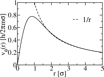
Figure 1: The left panel shows the column density profile of a vortex in the center of the trap. The central density drops about $47\%$ from its ground state value. The right panel shows the velocity distribution.

Using the wave function in Eq. (4), one can calculate the number density and the current density. The number density is defined as

$$\rho({\bf r})=\left(\prod_{i=1}^{\tilde{N}}\int d{\bf r}_{i}\right)\Psi^{*}\left[\sum_{j=1}^{{\tilde{N}}}\delta({\bf r}-{\bf r}_{j})\right]\Psi\;.$$ (10)

Since the density is independent of the azimuthal angle by symmetry, I can perform an angular average, and rewrite the integrand as a function of $\Delta\theta_{0}$. The radial profile of the number density is

$$\rho(r)=\frac{2{\tilde{N}}}{\pi R^{2}}\left(1-\frac{r^{2}}{R^{2}}\right)\int d^{2}{\bf r}^{\prime}_{0}\int d^{2}{\bf r}_{0}\left[S({\bf r}_{0},{\bf r}^{\prime}_{0})\int_{0}^{2\pi}\frac{d\theta}{2\pi}e^{i(\phi-\phi^{\prime}+\Delta\theta_{0})}\right],$$ (11)

where

$$S({\bf r}_{0},{\bf r}^{\prime}_{0})=f(r_{0})f(r^{\prime}_{0})e^{i{\tilde{N}}\Delta\theta_{0}}\langle\Psi_{\rm F}^{*}({\bf r}^{\prime}_{0})|\Psi_{\rm F}({\bf r}_{0})\rangle\;.$$ (12)

The angular average integral in Eq. (11) can be worked out explicitly as a combination of elliptic integrals.[16] The rest integrals can then be carried out numerically. In order to compare with the experimental result, I use the parameters in Ref. Madison00. The scattering length for ⁸⁷Rb is $5.45$ nm.[19] The frequency of the harmonic trap in the transverse direction is $\omega_{\perp}/2\pi=219$ Hz, and in the longitudinal direction is $\omega_{z}/2\pi=11.7$ Hz. For $10^{5}$ atoms, the maximum transverse size is $R=2.6\,\mu$m, and the central density for the ground state is about $n(0)=177\,\mu$m^-3. However, one has to find the effective length scale $\sigma$ in the two-dimensional theory from the parameters in three dimensions. Since $\sigma$ determines the size of the vortex core, a reasonable estimation is the healing length $\xi$. For a uniform gas, the healing length is given by $\xi=(8\pi na)^{-1/2}$, which is about $0.2\,\mu$m if the central density $n(0)$ is used. In units of this effective length scale, $\sigma\approx\xi$, the transverse size of the condensate is about $R/\sigma\approx 13$. I have carried out a calculation for $R/\sigma=15$, and the normalized density profile is shown in Fig. 1. The radial dependence of the condensate wave function has been changed from the pure two-dimensional profile $(1-r^{2}/R^{2})$ to the column density of a three-dimensional condensate $(1-r^{2}/R^{2})^{3/2}$.

One can compute the current density in a similar way. The azimuthal current density is defined as

$$J_{\theta}({\bf r})=\Im\left\{\frac{\hbar}{m}\left(\prod_{i=1}^{\tilde{N}}\int d{\bf r}_{i}\right)\Psi^{*}\left[\sum_{j=1}^{\tilde{N}}\delta({\bf r}-{\bf r}_{j})\frac{1}{r}\frac{\partial}{\partial\theta}\right]\Psi\right\}\;.$$ (13)

The radial distribution of the azimuthal velocity, $v_{\theta}(r)=J_{\theta}(r)/\rho(r)$, is also shown in Fig. 1 together with the velocity profile $\hbar/mr$ of a singular vortex line. In conclusion, a many-body wave function incorporating quantum fluctuations is presented to describe a vortex in a BEC. The calculated particle density at the vortex axis is finite, and agrees quantitatively with the experimental observation. The finite density at the vortex axis cannot be described by the GP equation, and manifests the quantum depletion.

References

- [1] M. H. Anderson, J. R. Ensher, M. R. Matthews, C. E. Wieman, and E. A. Cornell, Science 269, 198 (1995).
- [2] C. C. Bradley, C. A. Sackett, J. J. Tollett, and R. G. Hulet, Phys. Rev. Lett. 75, 1687 (1995).
- [3] K. B. Davis, M.-O. Mewes, M. R. Andrews, N. J. van Druten, D. S. Durfee, D. M. Kurn, and W. Ketterle, Phys. Rev. Lett. 75, 3969 (1995).
- [4] D. G. Fried, T. C. Killian, L. Willmann, D. Landhuis, S. C. Moss, D. Kleppner, and T. J. Greytak, Phys. Rev. Lett. 81, 3811 (1998).
- [5] J. E. Williams and M. J. Holland, Nature (London) 401, 568 (1999).
- [6] M. R. Matthews, B. P. Anderson, P. C. Haljan, D. S. Hall, C. E. Wieman, and E. A. Cornell, Phys. Rev. Lett. 83, 2498 (1999).
- [7] K. W. Madison, F. Chevy, W. Wohlleben, and J. Dalibard, Phys. Rev. Lett. 84, 806 (2000).
- [8] N. N. Bogoliubov, J. Phys. (USSR) 11, 23 (1947).
- [9] E. P. Gross, Nuovo Cimento 20, 454 (1961).
- [10] L. P. Pitaevskii, Zh. Eksp. Teor. Fiz. 40, 646 (1961) [Sov. Phys. JETP 13, 451 (1961)].
- [11] E. Timmermans, P. Tommasini and K. Huang, Phys. Rev. A 55, 3645 (1997).
- [12] E. Braaten and A. Nieto, Phys. Rev. B 56, 14745 (1997).
- [13] A. L. Fetter, Phys. Rev. Lett. 27, 986 (1971); A. L. Fetter, Ann. Phys. (N.Y.) 70, 67 (1972).
- [14] D. L. Hill and J. A. Wheeler, Phys. Rev. 89, 1102 (1953).
- [15] R. E. Peierls and J. Yoccoz, Proc. Roy. Soc. A 70, 381 (1957); R. E. Peierls and D. J. Thouless, Nucl. Phys. 38, 154 (1962).
- [16] J.-M. Tang, cond-mat/9812438.
- [17] Sir W. Thomson, Phil. Mag. 10, 155 (1880).
- [18] R. P. Feynman, in Progress in Low Temperature Physics, edited by C. J. Gorter (Elsevier Science Publishers B.V., Amsterdam, 1955), Vol. 1, Chap. 2, pp. 17–53.
- [19] P. S. Julienne, F. H. Mies, E. Tiesinga, and C. J. Williams, Phys. Rev. Lett. 78, 1880 (1997).