Shot Noise Suppression at 2D Hopping

Abstract

We have used Monte Carlo simulation to calculate the shot noise intensity $S_{I}(\omega)$ at 2D hopping using two models: a slanted lattice of localized sites with equal energies and a set of localized sites with random positions and energies. For wide samples we have found a similar dependence of the Fano factor $F\equiv S_{I}(0)/2eI$ on the sample length $L$: $F\propto L^{-\alpha}$ where $\alpha=0.85\pm 0.02$ and $\alpha=0.85\pm 0.07$ in uniform and random models, respectively. Moreover, at least for the uniform model, all the data for $F$ as the function of sample length $L$ and width $W$ may be presented via a single function of the ratio $W/L^{\beta}$, with $\beta=2\alpha-1\approx 0.7$. This relation has been interpreted using a simple scaling theory.

Shot noise at electron transport has been the subject of intensive experimental and theoretical research lately (for a recent review see, e.g., Ref. [1]), because it may provide important information about nonequilibrium properties of conductors, unavailable from other transport characteristics. Another motivation for studies of shot noise is its direct relation to electric charge discreteness. Namely, the smallness of the spectral density of current fluctuations at low frequency, $S_{I}(0)$, in comparison with the Schottky value of $2eI$, is a necessary condition for quasi-continuous charge transfer [2, 3]. Such “sub-electron” transfer through conductors with sufficiently high resistance $R$ and low stray capacitance $C$ may make possible several resistively-coupled single-electron devices insensitive to background charge randomness [4]. In this context, hopping conductors are very promising, so that the development of understanding of shot noise in such conductors seems to be an important task.

However, though the basic theory of hopping conductivity is well developed [5], until recently little had been known about noise at hopping. Few publications we were aware of had been devoted to narrowband, $1/f$-type noise (see, e.g., Ref. [6] and references therein) rather than broadband fluctuations such as shot noise. This is why in the recent work of our group [7] a detailed theoretical study of broadband current fluctuations at 1D hopping was carried out (on the foundation of prior important work on statistics of the so-called Asymmetric Simple Exclusion Process (ASEP) model [8]).

For uniform, linear 1D arrays the low-frequency noise depends on the boundary conditions (namely, the filling factors $f_{L},f_{R}$ of the edge sites) and may or may not be dominated by boundary bottlenecks. In the former case, the Fano factor $F=S_{I}(0)/2eI$ tends to a finite value of the order of 1 (e. g., for $f_{L}=f_{R}=f$, $T=0$ and negligible Coulomb interaction, $F=|1-2f|$) i.e., shot noise suppression is insignificant. In the absence of boundary bottlenecks (e. g., if $f_{L}=f_{R}=1/2$), the Fano factor tends to zero at large number of hops $N$, but only as $N^{-1/2}$, i.e. much slower than in 1D arrays of tunnel junctions where $F=1/N$ far enough from the Coulomb blockade threshold [3, 7]. (This behavior has been explained [7] using a simple scaling theory which also explains other features, i.e. the frequency dependence $S_{I}(\omega)\propto\omega^{-1/3}$ in an intermediate frequency range.) Nonuniformity of 1D hopping systems decreases the noise suppression, bringing the Fano factor closer to the Schottky value $F=1$.

The goal of this paper is to show that the ability of electrons to circumvent transport bottlenecks at 2D hopping leads to a qualitatively different situation. Namely, in sufficiently long and broad samples the shot noise may be suppressed quite considerably:

$$F\propto L^{-\alpha},$$ (1)

where $L$ is the conductor length and $\alpha\approx 0.85$, even in ultimately nonuniform conductors.

We have employed the usual Monte-Carlo simulation technique (see, e.g., Ref. [7]) to analyze two different models, so far both without Coulomb interaction and at vanishing temperature:

- Model A: hopping between sites with random localization energies, randomly distributed over a 2D sample, and

- Model B: hopping on a uniform, slanted lattice without site energy fluctuations.

In both models, each site may be occupied by just one electron, and the rate of (inelastic) transitions between the sites is described by the usual formula (see, e.g., Eq. (4.2.17) in Ref. [5]):

$$\Gamma_{i\rightarrow j}=A\,\frac{\epsilon_{ij}}{1-\exp(-\epsilon_{ij}/T)},$$ (2)

corresponding to the constant density of phonon states. Here $\epsilon_{ij}$ is the electron energy gain during the hop $i\rightarrow j$; in the absence of Coulomb interaction between electrons this gain can be expressed as

$$\epsilon_{ij}=(\epsilon_{i}-\epsilon_{j})-eE(x_{i}-x_{j}),$$ (3)

where $E$ is an external electric field applied along the $x$ axis. For relatively short samples special care should be taken to adequately describe electron transfer between the electrodes and the edge localized sites. After experimenting with various options, we have concluded that the same expression (2) may be used to describe this transfer, without creating unphysical bottlenecks at the electrode-sample interfaces [9].

In our main Model A, single-particle site energies $\epsilon_{i}$ are distributed randomly within a broad energy band, with a constant 2D density of states $D$, and site positions ${x_{i},y_{i}}$ are randomly distributed within a rectangular sample of length $L$ and width $W$. The rate amplitude $A$ is an exponential function of the intersite distance $r_{ij}$:

$$A=A_{0}\exp(-r_{ij}/a),$$ (4)

where $a$ is half of the localization radius. All the results have been averaged not only over a sufficiently long time period, but also over a set of random samples with the same global dimensionless parameters $L/a$, $W/a$, and $eEDa^{3}$ (parameter $A_{0}$ just determines the scale $I_{0}=eA_{0}W/Da^{3}$ of the total current). Such averaging requires considerable computer resources; the calculations have been performed on IBM SP parallel supercomputer.

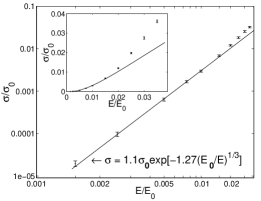
FIG. 1.: The nonlinear dc conductivity $\sigma=I/WE$ (normalized by $\sigma_{0}=I_{0}/WE_{0}$), as a function of electric field $E$ for Model A. The straight line is the analytical fit discussed in the text. Inset: the same data on a linear scale.

Figure 1 shows the numerically calculated nonlinear dc conductivity $\sigma=I/WE$ as a function of electric field $E$ for sufficiently long and wide samples. Depending on $E$, we have simulated samples of area $L\times W$ ranging from $120a\times 30a$ up to $300a\times 120a$ to keep the number of “active” sites $N_{s}\sim 1500$ approximately constant (the growing error bars at lower $E$ are due to larger fluctuations from sample to sample). The absence of significant dependence of $\sigma$ on the sample size was being checked. For low electric fields $E\lesssim 0.02E_{0}$ ($E_{0}=1/eDa^{3}$) the current follows closely the dependence $I/E\propto\exp[-C(E_{0}/E)^{1/3}]$ expected for 2D variable range hopping [5, 10] in the activationless (“high field”) regime. The best fit (straight line in Fig. 1) gives the numerical constant $C\approx 1.27$. (This number is to be compared with the value $C=1.02$ following from analytical calculations in Ref. [11].) The minor deviation from the analytical dependence at $E\gtrsim 0.02E_{0}$ is possibly due to multiple, well-branched percolation paths which are not considered in the usual theoretical treatment of high field hopping.

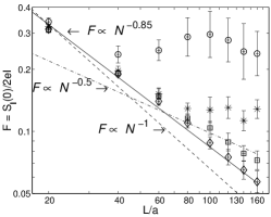
FIG. 2.: Dependence of the Fano factor $F$ in Model A (averaged over 32 sample realizations) on the sample length $L$ for $E=0.035E_{0}$. Circles: $W=5a$, asterisks: $W=10a$, squares: $W=20a$, diamonds: $W\rightarrow\infty$. Error bars show the standard deviation of the mean.

Figure 2 shows the Fano factor (averaged over 32 sample realizations) as a function of the sample length for $E=0.035E_{0}$ and for tree values of sample width: $W=5a$ (circles), $W=10a$ (asterisks) and $W=20a$ (squares). At this field the average hop length is $\overline{r}\approx 3.3a$ (with r.m.s. projections $r_{x}\approx 3.1a$, $r_{y}\approx 1.9a$) so that the factor $\exp(-\overline{r}/a)$ is still small. Most importantly, we see that shot noise is suppressed considerably ($F\ll 1$) in wide and long samples. As a function of the sample length $L$ at fixed width $W$, the average Fano factor first decreases following Eq. (1) (solid line in Fig. 2) and then at certain length deviates up from this dependence. The deviation starts at larger $L$ for wider samples. For narrower samples one can see the saturation of the average Fano factor at large $L$; simultaneously the width of the Fano factor distribution grows significantly. The average Fano factor also decreases with the sample width at fixed length, obviously saturating at large $W$ since the electron transport in remote parts of a very wide sample is uncorrelated. Having performed the calculations at fixed length for several widths (not all the results are shown in Fig. 2) we have extrapolated the Fano factor dependence to infinitely wide 2D samples. As a function of $L$, these results (shown in Fig. 2 by diamonds) closely follow Eq. (1) with $\alpha=0.85\pm 0.07$. The power-law dependence $F(L)$ has been observed within one order of magnitude range of $L$. The longer samples have not been studied due to computer limitations (as an example, calculations of a single point $L=160a$, $W=20a$ in Fig. 2 has required 380 hours of total CPU time).

In order to verify the shot noise suppression for larger set of lengths and widths, we have used the simplified Model B in which $(N-1)\times M$ localized sites with equal energies are arranged on a uniform slanted square lattice (see inset in Fig. 3) [12]. In accordance with Eq. (2), at $T=0$ the transport is unidirectional, and transfer rates $\Gamma$ between all the internal neighboring sites are equal. For the links from the left electrode to the nearest internal sites we have selected the rates $2\Gamma f_{L}$ (the factor of 2 reflects two “channels” per internal site) while the rates of hopping onto the right electrode are $2\Gamma(1-f_{R})$. For the numerical analysis we have chosen the case $f_{L}=f_{R}=0.5$ in which, similarly to 1D model, there are no boundary bottlenecks. Since Model B does not require averaging over different random realizations, it may be studied with much better accuracy using the same computer resources.

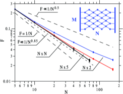
FIG. 3.: Fano factor dependence on the length $N$ for hopping on a uniform slanted square lattice (Model B, inset) with width $M$ equal to 2, 5, and $N$.

Figure 3 shows the Fano factor as a function of the array length $N$ for several values of width $M$. Again, we see a strong shot noise suppression. For sufficiently wide samples the suppression follows Eq. (1) (where now $L$ should be replaced by $N$), with similar exponent as in the wide random samples: $\alpha=0.85\pm 0.02$. On the other hand, for fixed $M$ and sufficiently long $N$ the suppression power approaches $0.5$, i.e. the same value as for 1D hopping [7].

There is numerical evidence (see Fig. 4), as well as scaling arguments (see below), that for $N\gg 1$ and $M\gg 1$ the crossover between these two asymptotic laws may be parameterized in the following way:

$$F(N,M)=N^{-\frac{1}{2}}M^{-\frac{1}{2}}g(N^{\beta}/M),$$ (5)

where $\beta=0.70\pm 0.04$, and the function $g(x)$ is shown in Fig. 4:

$$g(x)\propto\left\{\begin{array}[]{ll}const,&x\gg 1\\ x^{-1/2},&x\ll 1.\end{array}\right.$$ (6)

Checking if the data from Fig. 2 for the random Model A may also be collapsed on the similar universal curve we have found a reasonable fit for relatively wide samples (see inset in Fig. 4) for the following replacements: $N=L/5.9a$, $M=W/11a$ (for the particular field $E=0.035E_{0}$).

We will start the interpretation of our findings from the uniform Model B. Similarly to the 1D ASEP model [8], in the absence of lateral boundary effects due to finite $M$, and at $f_{L}=f_{R}=f$ the probability of any charge configuration is expected to be the same as if each site had independent occupation with probability $\rho=f$ [13]. As a result, dc current between any two neighboring sites should equal $\Gamma\rho(1-\rho)$, so the total dc current is

$$I=2M\Gamma\rho(1-\rho).$$ (7)

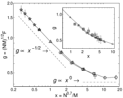
FIG. 4.: The data from Fig. 3 (circles: $M=2$, triangles: $M=5$, and stars: $M=N$) collapsed onto universal curve $g(x)$ using parameterization $x\equiv N^{0.7}/M$ and $g\equiv(NM)^{1/2}F$. Lines connecting points are just guides for the eye. The inset shows the same data with added points for $W=20a$ (squares) from Fig. 2 using the rescaling $N=L/5.9a$ and $M=W/11a$.

Following the arguments of Ref. [7] we obtain only a minor suppression of low-frequency shot noise, $F\approx|1-2\rho|$, in the case $\rho\neq 0.5$ (the noise significantly decreases at frequencies $\omega\gtrsim\omega_{l}\sim\Gamma|1-2\rho|/N$). However, when the coupling with electrodes is strong enough, $f_{L}\geq 0.5$, $f_{R}\leq 0.5$, the half-filling is expected inside the array, $\rho=0.5$, and the Fano factor can indefinitely decrease with the array length $N$. In this case, for sufficiently large $N$ (narrow array) we may repeat all 1D scaling arguments of Ref. [7] based on Eq. (7), and arrive at the following estimates:

$$F\sim(NM)^{-1/2},\,\,\,\omega_{l}\sim\Gamma N^{-3/2}M^{-1/2},$$ (8)

for the Fano factor and the saturation frequency $\omega_{l}$, above which the dependence $S_{I}(\omega)/2eI\sim(\omega/\Gamma)^{-1/3}N^{-1}$ is expected.

Obviously, this result should eventually fail if we start increasing the width $M$ for fixed $N$, because $F$ cannot depend on $M$ in the limit of wide array (since the transport in remote parts of the array is uncorrelated and so both $S_{I}$ and $I$ are additive). Denoting the crossover width as $M_{0}$ we get the estimate $F\sim(NM_{0})^{-1/2}$ for wide arrays. It would be natural to expect $M_{0}\propto N$, however, the numerical results (Fig. 3) indicate the power-law dependence, $M_{0}\propto N^{\beta}$, with $\beta$ being a phenomenological parameter. If this assumption is true, we obtain the following estimates:

$$F\sim N^{-(1+\beta)/2},\,\,\,\omega_{l}\sim\Gamma N^{-(3+\beta)/2},$$ (9)

for wide arrays, $M\gg N^{\beta}$. Our numerical result, $\alpha=0.85\pm 0.02$, then leads to the value $\beta=2\alpha-1=0.7\pm 0.04$. For intermediate widths it is natural to suggest that the crossover is governed by some function of the ratio $x\equiv N^{\beta}/M$ alone. Thus we recover the behavior described by Eqs. (5)–(6) and illustrated by Fig. 4. [Actually, at this stage we cannot rule out the possibility that the function $g$ in Eq. (5) also has a weak dependence on $M$ that would lead to either smoothing or sharpening of the curve in Fig. 4, leaving however the asymptotes (6) intact.]

If we apply the same scaling arguments which have led to Eq. (9), to smaller blocks [7] of size $N_{\omega}\times N_{\omega}^{\beta}$, we obtain the noise frequency dependence

$$S_{I}(\omega)/2eI\sim\omega^{-\gamma}N^{-1},\,\,\,\gamma\equiv(1-\beta)/(3+\beta),$$ (10)

for wide arrays at intermediate frequencies, $\omega_{l}\ll\omega\ll\Gamma$.

This power-law dependence, $S_{I}(\omega)\propto\omega^{-0.08}$, was confirmed numerically with the accuracy of the exponential factor about $\pm 0.007$. The same frequency dependence should be expected for the narrow arrays, $M\ll N^{\beta}$, at frequencies higher than $\sim\Gamma M^{-(3+\beta)/2\beta}$, while at lower frequencies $S_{I}(\omega)\propto\omega^{-1/3}$, as discussed above.

Now, let us turn back to our main, random Model A. According to the percolation picture of hopping [5], the conductivity of a sample is determined by a “percolation cluster”, essentially a network of sites connected by the most probable hop paths. The percolation cluster may be divided into blocks of a certain size, such that the aggregate characteristics of each block (e.g. the average current) are nearly equal, even though inside each block the sample is highly (exponentially) nonuniform. Average block size in the transport direction for the random model A may be determined by mapping 2D hopping in disordered wide samples onto the uniform model B, for $M>N$, where the shot noise suppression was found to be similar. If this interpretation is valid, then the ratio $L/N=5.9a$ obtained from the mapping should be comparable to the correlation length $L_{c}\sim\overline{r}(\overline{r}/a)^{\nu}\sim 3.3a$ [14]. We believe these numbers are reasonably consistent.

On the other hand, the model A behavior in narrow samples ($W\lesssim 10a$) is quite different from that in the uniform model: instead of going down with growing $N$, the Fano factor saturates. Simultaneously, the statistics of $F$ becomes much wider. This behavior is very natural, since if the sample is narrower than the block size (for our value of electric field, about $10a$), the exponentially broad distribution of hopping paths within the block is revealed and is mapped onto the properties of the sample as a whole.

Our results for wide samples are in good agreement with data from a recent experiment [15] in which shot noise at hopping was measured in $p-$type SiGe quantum wells. Actually, the experimental I-V curve significantly differs from that in our Model A. However, our result (1) for $F$ seem more general. For wide samples with two different lengths $L_{1}=2\mu$m and $L_{2}=5\mu$m the Fano factor was measured [15] to equal $F_{1}=0.43$ and $F_{2}=0.2$, respectively. This corresponds to Eq. (1) with $\alpha=0.84$, the value which is virtually equal to our result $\alpha=0.85$. Such perfect agreement is possibly just a coincidence, since so far only two experimental points are available. Evidently, it would be valuable to have more experimental data, in order to verify the shot noise suppression power $\alpha=0.85$.

In conclusion, we have numerically investigated shot noise suppression at 2D hopping in random samples as well as in uniform arrays. Very similar shot noise suppression has been found for both models for wide and long samples. At 2D hopping the Fano factor decreases with the sample length as $F\propto 1/L^{0.85}$. This suggests that shot noise suppression at 2D hopping is insensitive to details of the hopping process, e.g., the energy dependence of the hopping rate. If this surmise is true, the Fano factor should not be a very strong function of temperature. It may, however, be substantially altered by Coulomb interaction of hopping electrons, as in the 1D case [7]. Our next plans are to explore the effects of both these factors.

Fruitful discussions with V. Kuznetsov and generous help by J. Wells are gratefully acknowledged. The work was supported in part by the Engineering Research Program of the Office of Basic Energy Sciences at the Department of Energy. The authors also acknowledge the use of the Oak Ridge National Laboratory IBM SP computer, funded by the Department of Energy’s Offices of Science and Energy Efficiency program.

REFERENCES

- [1] Ya. M. Blanter and M. Büttiker, Physics Reports 336, 2 (2000).
- [2] D. V. Averin and K. K. Likharev, in: Mesoscopic phenomena in solids, ed. by B. Altshuler et al. (Elsevier, Amsterdam, 1991), Ch. 6.
- [3] K. A. Matsuoka and K. K. Likharev, Phys. Rev. B 57, 15613 (1998).
- [4] K. K. Likharev, Proc. IEEE 87, 606 (1999); A. N. Korotkov, Int. J. Electron 86, 511 (1999).
- [5] B. I. Shklovskii and A. L. Efros, Electronic properties of doped semiconductors (Springer, Berlin, 1984).
- [6] Sh. Kogan, Phys. Rev. B 57, 9736 (1998).
- [7] A. N. Korotkov and K. K. Likharev, Phys. Rev. B 61, 15975 (2000).
- [8] B. Derrida and E. Domany, J. Stat. Phys. 69, 667 (1992).
- [9] Physically, this transfer may be dominated by elastic tunneling for which Eq. (2) is not quite adequate. Our study, however, was focused on long samples () for which this difference is unimportant.
- [10] M. Pollak and I. Riess, J. Phys. C: Solid State Phys. 9, 2339 (1976.)
- [11] R. B. Thompson and M. Singh, Phil. Mag. B 75, 293 (1997).
- [12] The uniform model on the usual (non-slanted) 2D array cannot give an adequate presentation of hopping in random systems, since it fails to describe any hops other than exactly along the applied field, and hence may be exactly reduced to the uniform 1D model studied in Ref. [7].
- [13] This result becomes exact even for finite at the cyclic boundary conditions in the direction normal to the field.
- [14] B. I. Shklovskii, Fiz. Tekh. Poluprovodn. 10, 1440 (1976) [Sov. Phys. Semicond. 10, 855 (1976)].
- [15] V. V. Kuznetsov, E. E. Mendez, E. T. Croke, X. Zuo, and G. L. Snider, Phys. Rev. Lett. 85, 397 (2000)