Local Reorientation Dynamics of Semiflexible Polymers in the Melt

Abstract

The reorientation dynamics of local tangent vectors of chains in isotropic amorphous melts containing semiflexible model polymers was studied by molecular dynamics simulations. The reorientation is strongly influenced both by the local chain stiffness and by the overall chain length. It takes place by two different subsequent processes: A short-time non-exponential decay and a long-time exponential reorientation arising from the relaxation of medium-size chain segments. Both processes depend on stiffness and chain length. The strong influence of the chain length on the chain dynamics is in marked contrast to its negligible effect on the static structure of the melt. The local structure shows only a small dependence on the stiffness, and is independent of chain length. Calculated correlation functions related to double-quantum NMR experiments are in qualitative agreement with experiments on entangled melts. A plateau is observed in the dependence of segment reorientation on the mean-squared displacement of the corresponding chain segments. This plateau confirms, on one hand, the existence of reptation dynamics. On the other hand, it shows how the reptation picture has to be adapted if, instead of fully flexible chains, semirigid chains are considered.

For submission to Macromolecules

1 Introduction

Modern double-quantum nuclear magnetic resonance (NMR) experiments aim to understand the microscopic dynamics of polymer segments in the melt.[1] The polymer dynamics is most often described by either the Rouse[2] or the reptation[3, 4] model depending on chain length. Both models, however, take the architecture of a specific polymer into account only via the so-called Kuhn length. These local features are summarized into $C_{\infty}=\frac{\langle\vec{R}^{2}\rangle}{Nl_{b}^{2}}$, the ratio between the mean squared end-to-end distance $\langle\vec{R}^{2}\rangle$ and the number of monomers $N$ (multiplied with the squared bond length $l_{b}^{2}$). Statics and dynamics are thus renormalized onto a Gaussian bead-spring chain of larger but fewer beads of the size of the Kuhn length $l_{K}=\frac{\langle\vec{R}^{2}\rangle}{Nl_{b}}$. Experimentally, however, there is a qualitative difference between fully flexible polymers like poly-(dimethyl-siloxane) (PDMS)[5] and moderately stiff systems like poly-(butadiene) (PB)[6] when it comes to the reorientation of chain segments. These differences remain after both polymers have been appropriately renormalized onto Gaussian chains. The PB system shows unusual dynamics which has been taken as an indication of local order[6], whereas the PDMS data is quite successfully described by the standard reptation picture[5]. From the shape of reorientation auto-correlation functions a relatively high degree of residual structural order in the presence of entanglements has been deduced for PB. The experimental data, however, cannot be interpreted without model assumptions. Here, simulations which are validated against experimental raw data may contribute to a better understanding.[7]

Molecular dynamics simulations are widely applied to study the dynamics of simplified polymer models in solution[8, 9] and the melt[10, 11, 12, 13, 14, 15, 16]. To date, only simple models are capable of investigating dynamics of long entangled polymer chains in the melt to a satisfactory degree of accuracy. Models that allow for atomistic details are limited to shorter times and to fewer and shorter chains.[17, 18, 19, 20]

Recently, we showed that the static local mutual orientation of neighboring chains depends on chain stiffness in the amorphous melt, whereas the chain length has no influence on local static properties.[15, 21] In the present contribution, we now extend our investigations to the dynamics of entangled and unentangled melts of polymer chains with local stiffness. In the following section, the polymer model is shortly recapitulated and details of the simulated systems are described. In the main part (Section 3), reorientation correlation functions are analyzed and compared to theoretical considerations and experiments. Section 4 relates static chain packing and dynamic chain reorientation observables.

2 Model and Computational Details

We performed polymer melt simulations using Brownian dynamics (BD) of a widely used and well characterized generic polymer model[10, 12, 14] with added local stiffness.[21] All monomers interact via a truncated and shifted, therefore purely repulsive, Lennard-Jones potential (Weeks-Chandler-Andersen, WCA, potential[22])

$$V_{WCA}(r)=4\epsilon\left[\left(\frac{\sigma}{r}\right)^{12}-\left(\frac{\sigma}{r}\right)^{6}+\frac{1}{4}\right],\;r<\sqrt[6]{2}\sigma\;.$$ (1)

Neighbors on the chain are connected by a finitely extensible non-linear elastic (FENE) potential which is used for computational efficiency

$$V_{FENE}(r) = -\frac{\alpha}{2}\frac{R^{2}}{\sigma^{2}}\ln\left(1-\frac{r^{2}}{R^{2}}\right),$$ (2)

$$r<R = 1.5\sigma\;,\quad\alpha=30\epsilon\;.$$

This yields, together with the WCA-potential, an anharmonic spring. Most of our systems have an additional three-body potential to stiffen the chain locally

$$V_{bend}=b\left(1-\frac{\vec{r}_{i-1,i}\cdot{\vec{r}_{i,i+1}}}{r_{i-1,i}r_{i,i+1}}\right)\;,\quad\vec{r}_{ij}:=\vec{r}_{j}-\vec{r}_{i}\;.$$ (3)

For details of the implementation and parallelization, see ref. 23. Throughout this work, reduced units are used with mass $m$, bead diameter $\sigma$, and the strength of the WCA potential $\epsilon$ set to unity. The time unit is $t^{*}=\sigma\sqrt{\frac{m}{\epsilon}}$. Temperature is measured in units of $\epsilon$ by setting Boltzmann’s constant $k_{B}=1$. The average bond length is $l_{b}=0.97\sigma$ so that the beads overlap only slightly.

Systems of up to 1000 chains of length $N$ monomers ranging from 5 to 1000 were simulated at melt density ($\rho^{*}=0.85\sigma^{-3}$) and temperature $T^{*}=1$. The Brownian dynamics algorithm is mainly used to maintain this temperature. Additionally, it has been shown to be very efficient for our model [12]. The monomer friction coefficient of 0.5 inverse time units used here means that only processes on a time scale well above one of our time units have a meaningful dynamics. The persistence lengths $l_{p}$ defined via the decay of the bond direction correlation function along the chain backbones varied from one bond length up to 5 bond lengths.

$$\Big{\langle}\vec{u}(0)\vec{u}(l)\Big{\rangle}=e^{-l/l_{p}},$$ (4)

The distance $l$ is measured along the contour of the chain. The persistence length is related to the Kuhn length (Section 1) in the worm-like chain model by $l_{p}=\frac{1}{2}l_{K}$.[4] In the simulations, $l_{p}$ is controlled by choosing appropriate values of $b$ in Eq. 3. Hence, throughout this article we refer to systems of different stiffness with their $l_{p}$ rather than the corresponding $b$. The most flexible system ($l_{p}\approx l_{b}$) has no intrinsic stiffness, only the excluded-volume interaction leads to its persistence length being non-zero. The persistence length increases weakly with chain length due to end effects.[21] The values indicated here are the limits for long chains. For $N\geq 10$ the persistence length is much shorter than the contour length. An overall Gaussian behavior is therefore expected and confirmed by the characteristic ratio $\lim_{N\to\infty}\frac{R^{2}_{end-end}}{R^{2}_{gyr}}\approx 6$.[21] Note that the model would show a nematic liquid crystalline phase if the bending stiffness was increased far above $l_{p}=5$.[24]

All chains of length up to 75 and all flexible chains $(l_{p}=1)$ relaxed fully, as evidenced by the decay of all the Rouse modes. To cut down necessary equilibration times, the longer chains (or chains of greater stiffness) were initialized as non-reversal random walks whose local structure was estimated from simulations of shorter chains: In the setup configuration a monomer $i$ and its second neighbor $i+2$ are not allowed to approach closer than a certain distance. This setup procedure reduces the equilibration time substantially while producing useful configurations.[12]

The end-to-end distance and the gyration radius changed then only very slightly in the initial stage of the simulation. Their equilibrium values as a function of stiffness were already presented in reference 21 together with other static observables like structure functions, pair distribution functions and local chain orientation correlation functions. Some of this data is included in section 4. It is not yet possible to simulate the “slowest” systems (e.g. $l_{p}=5,\quad N=1000$) until the final regime of free diffusion is reached. Still, we trust that even this system is sufficiently equilibrated for the purpose under study.

Table 1 gives an overview of the simulated systems with their respective Rouse times and simulated times. We are aware that for non-flexible polymers the Rouse modes are no longer the true eigenmodes (see section 3). Still, the Rouse time is useful as an estimate of the relaxation time. For chains of equal length, the Rouse time $\tau_{R}$ would increase linearly with chain extension, i.e. $l_{p}$, if the friction due to neighboring chains were constant.[4] However, the relaxation times increase even stronger (Table 1 and Figure 1). Similarly, for the non-flexible chains ($l_{p}>1$), the increase of $\tau_{R}$ with $N^{2}$ as expected from the Rouse model is no longer observed. The slowdown is stronger, indicating an earlier onset of entanglement influence with increasing persistence length (Table 1).

$$\begin{array}[]{|D{.}{.}{-1}|r|r|r|r|D{.}{.}{-1}|}\hline\cr l_{p}$&N&N_{c}&t_{sim}&\tau_{R}&6DN$\\ \hline\cr.4$&5&1000&30000&(40)&0.44$\\ 3.0$&5&1000&30000&(62)&0.42$\\ 5.0$&5&1000&30000&(88)&0.38$\\ \hline\cr.0$&10&500&30000&140&0.43$\\ .4$&10&500&30000&170&0.43$\\ 3.0$&10&500&30000&290&0.35$\\ 5.0$&10&500&33000&(730)&0.27$\\ \hline\cr.4$&13&500&25000&290&0.35$\\ \hline\cr.4$&15&500&25000&370&0.35$\\ \hline\cr.4$&17&500&67000&590&0.30$\\ 3.0$&17&500&30000&1070&0.27$\\ 5.0$&17&500&30000&2600&0.21$\\ \hline\cr.4$&20&500&30000&780&0.29$\\ 3.0$&20&500&20000&1700&0.23$\\ 5.0$&20&500&25000&3700&0.19$\\ \hline\cr.0$&25&500&30000&900&0.42$\\ .4$&25&500&25000&1400&0.29$\\ 3.0$&25&500&63000&2900&0.20$\\ 5.0$&25&500&78000&6400&0.18$\\ \hline\cr.4$&30&500&25000&2000&0.26$\\ 3.0$&30&500&25000&5000&0.17$\\ \hline\cr 5.0$&35&500&53000&21000&$\\ \hline\cr.0$&50&500&20000&3500&0.31$\\ .4$&50&500&22000&8300&0.18$\\ 3.0$&50&500&70000&23000&0.10$\\ 5.0$&50&500&50000&43000&$\\ \hline\cr.4$&75&500&76000&27000&0.13$\\ \hline\cr.4$&200&500&300000&{}^{*}300000&$\\ 3.0$&200&500&350000&{}^{*}400000&$\\ 5.0$&200&500&700000&{}^{*}700000&$\\ \hline\cr.0$&350&120&1700000&530000&$\\ \hline\cr 5.0$&1000&250&60000&O(10^{7})&$\\ \hline\cr\end{array}$$

Table 1: Simulated systems: $l_{p}$: persistence length in monomers; $N$: chain length in monomers; $N_{c}$: number of chains, $t_{sim}$: Simulation times; $\tau_{R}$: Rouse times (obtained by exponential fit of the lowest 3 to 5 Rouse modes. ^∗ partly estimated), numbers in brackets for systems where chains are too short; $D$: center of mass diffusion constant (for the systems where free diffusion could be reached). Some data of the system with 120 chains of length 350 are also presented in ref. 16. The errors in $\tau_{R}$ are at most 5% and the errors in $6DN$ are about 0.01.

Figure 1: Increase of Rouse times with persistence length at $N=50$. The dashed line corresponds to an algebraic increase with $l_{p}^{1.54}$.

The very short chains ($N\leq 15$) allow an estimate of the diffusion coefficient of chains of a given stiffness, i.e. their mobility in the absence of entanglements. The diffusion coefficient does not decrease linearly with chain stiffness as would be expected from the Rouse model; for reptation this decrease is quadratic. As entanglement length we take the chain length for which the crossover from linear to quadratic takes place.[25, 26]

3 Chain Reorientation

3.1 Reorientation Correlation Function

The main purpose of this work is to investigate the reorientation dynamics of local chain segments in dense melts. This was studied by means of the auto-correlation function of the second Legendre polynomial $P_{2}$ of chain tangent vectors

$$C_{reor}(t)=\Bigg{\langle}\frac{1}{2}\Big{[}3(\vec{u}(t)\vec{u}(0))^{2}-1\Big{]}\Bigg{\rangle}=\Big{\langle}P_{2}[\vec{u}(t)\vec{u}(0)]\Big{\rangle}$$ (5)

As chain tangent vectors we take (normalized) vectors connecting neighboring beads

$$\vec{u}=\frac{\vec{r}_{i+1}-\vec{r}_{i}}{|\vec{r}_{i+1}-\vec{r}_{i}|}$$ (6)

unless noted otherwise. The second, rather than the first, Legendre polynomial is taken because its Fourier transform relates directly to NMR measurements ($T_{1}$ experiments) Also the double-quantum experiments aimed at the chain dynamics are related to this function (below).

3.1.1 Short-time behavior

For all systems investigated, we have found that the reorientation correlation function (Eq. 5) consists of two qualitatively different parts. For short times, its decay follows a power law (algebraic). At long times, the decay is exponential. All characteristics of the reorientation correlation function are influenced by the chain length $N$ and the chain stiffness $l_{p}$: the short-time part, the long-time part, the time at which the cross-over from algebraic to exponential behavior occurs and the function value at this point. We will see that the short-time regime is influenced more by stiffness, while the long-time regime shows a stronger dependence on chain length.

The influence of the chain architecture on the short-time behavior is illustrated in Fig. 2. Reorientation is slowed by increasing the stiffness at constant length (Fig. 2a) as well as by increasing the length at constant stiffness (Figs. 2b and  2c for $l_{p}=5$ and $l_{p}=1.4$, respectively). The more flexible chains and the shorter chains reach exponential behavior earlier. At the same time, the short-time algebraic process is more ”efficient” for the shorter and the more flexible chains, i.e. the reorientation correlation function has decreased to a smaller value when long-time exponential behavior sets in.

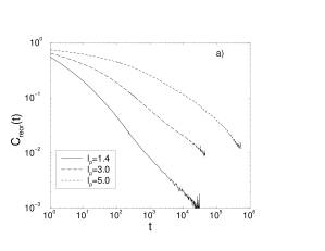
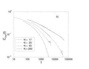
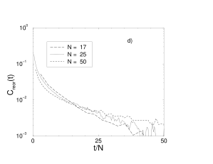
Figure 2: Short-time behavior of time dependent second Legendre polynomial of next neighbor vectors for different systems. a) $N=200$ different persistence lengths, b) $l_{p}=5$ different chain lengths, c) $l_{p}=1.4$ different chain lengths. d) System $l_{p}=1.4$ for very short times rescaled by $\frac{1}{N}$.

These findings can be understood if one attributes the short-time behavior to local dynamics and the long-time behavior to the relaxation of larger chain segments or, ultimately, to the rotational diffusion of entire chains. If the chains are flexible much of the reorientation can be achieved by local rearrangement, i.e. without the local tangent vector feeling that it is part of a long entangled chain. As stiffness increases, it hinders the reorientation on local scales, so the reorientation of the local tangent vector has to wait for some larger-scale reorientation which is exponential. The early crossover to exponential behavior and the apparently small efficiency of the short-time process for short chains, on the other hand, is due to a faster rotational diffusion of the entire chains, as they become shorter. The rotational diffusion begins to contribute substantially to the reorientation, before the local process can complete. Its time dependence is exponential according to e.g. the Debye model.[27]

If the Rouse model were strictly applicable the relaxation time of entire chains in the melt (Rouse time $\tau_{R}$) should scale with $N^{2}$. Hence, for constant stiffness the reorientation correlation functions belonging to different $N$ should coincide if the time axis is transformed $t\to t/N^{2}$. Instead, we find empirically that coincidence is achieved for $t\to t/N$ (Fig. 2d). This indicates that even for a small deviation from full flexibility ($l_{p}$=1.4) the Rouse model is not appropriate for the short-time relaxation, the local process being dominated by effects other than connectivity, e.g. stiffness. Additionally the “bead friction” enters which also increases sublinearly with stiffness.[26]

In contrast to the local dynamics, there is no chain length influence at all on local structural properties.[21]

As a general result, we note that, while the short-time process is influenced by both stiffness and chain length, the influence of stiffness is much stronger. (This can, for example, be seen by comparing Figures 2b and 2c.) It is, therefore, to be expected that also in experiments on real polymers the short-time regime will experience the influence from the chemical architecture of the polymer, whereas the chain length should be secondary.

3.1.2 Long-time behavior

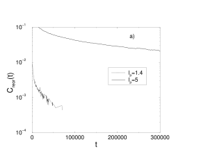
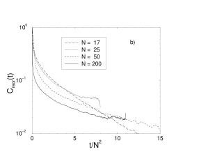
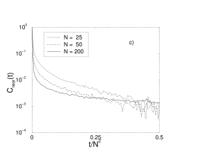
Figure 3: Late stage exponential decay of $C_{reor}(t)$ for different systems. Time is rescaled by $\frac{1}{N^{2}}$ to show differences to Rouse behavior. a)-c) as in Figure 2

The long-time tail of the reorientation correlation function is exponential to a reasonable approximation (Figure 3). The rate of decay depends – as the short-time behavior – on both chain stiffness (Fig. 2a) and chain length (Figs. 2b and c). The reorientation time of the exponential part $\tau_{reor}$ increases with both chain length $N$ and stiffness $l_{p}$ (Fig. 4). The dependence on $N$ is stronger than in the short-time regime, where an approximately linear increase with chain length was found (Figure 2d). This is expected because for larger scale processes the Rouse model should be appropriate and the overall chain relaxation characterized by the decay of all Rouse modes should scale with $N^{2}$. Therefore, the time axis is rescaled in Figures 3b and 3c to highlight the remaining deviation from Rouse behavior. As one approaches the entanglement regime (the entanglement lengths of the systems are compiled in Table 2), an even stronger increase with chain length is expected.

The reorientation time $\tau_{reor}$ (Figure 4) is much shorter than the time for the reorientation of entire long chains. Thus, one may suspect that in the case of long entangled chains, it is no longer important for the reorientation of a tangent vector, whether the entire chain reorients completely. Instead, the relaxation of a shorter part of the chain appears to be sufficient.

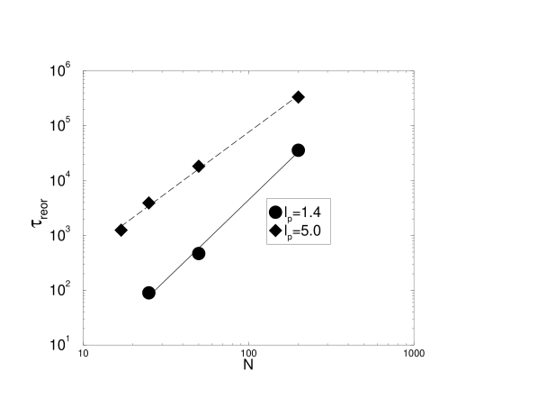
Figure 4: Reorientation times $\tau_{reor}$ of local segments as a function of chain length and stiffness. These are calculated from exponential fits to the long-time part of the reorientation correlation function Eq. 5. The dashed line indicates an increase with $N^{2.3}$ for $l_{p}=5$ whereas the solid line indicates $N^{2.9}$ for $l_{p}=1.4$.

$l_{p}$	$N_{e}$	$\tau_{e}$
1.0	32	1800
1.4	15	1300
3.0	8	1300
5.0	6	–

Table 2: Approximate entanglement lengths $N_{e}$ (in number of monomers) and respective times $\tau_{e}=\tau_{R}(N_{e})$ for the different persistence lengths.These were determined from the mean-squared displacements of chains.[12, 25] For $l_{p}=5$ the entanglement time is not defined.

This is in line with theoretical expectations: In the limit of infinitely long chains, the local segmental dynamics has to become independent of the chain length. The relaxation of a large but finite segment of the chain (a few entanglement lengths long) has to give enough freedom for the local reorientation to take place. This would only be different if the ends of the relevant segment were constrained for all times. We were able to corroborate these considerations by simulating an entangled melt of fully flexible chains ($N=350,\,l_{p}=1$) where the initial algebraic decay of $C_{reor}$ is very fast ($\approx 1800t^{*}$)[14] and effective in the sense that it reduces $C_{reor}(\tau_{e})$ to less than 0.01 before the long-time reorientation sets in. The decay time of the long-time process is about 5000$t^{*}$ which is the relaxation time of chain-segments of the length of about 60 monomers. This corresponds to about two entanglement lengths of the system[12], so we can deduce that, after completion of short-time relaxation, only relaxations on a length scale of up to the order of the entanglement length are relevant.

3.1.3 Reorientation of medium-size chain segments

It is also of interest to analyze the reorientation of longer chain segments. As the orientation vector of a segment of length $d$ we take the unit vector between two monomers whose indices on the chain differ by $d$

$$\vec{u}_{d}=\frac{\vec{r}_{i+d}-\vec{r}_{i}}{|\vec{r}_{i+d}-\vec{r}_{i}|}\;.$$ (7)

Thus $d=1$ represent the vectors connecting neighbors discussed up to now.

Figure 5: Reorientation of chain segments of different length $d$ for the system with length $N=200$ and persistence length $l_{p}=5$: $d$=1, 3, 5, 9, 11, 13, 19, 39, 79, 119 and 199 (end-end vector) from bottom to top.

$d$	$\beta$	$\frac{\tau_{reor}}{1000}$
1	0.055	269
3	0.087	272
5	0.115	276
9	0.172	283
11	0.202	286
39	0.533	335
199	0.796	558

Table 3: Fitted exponential decays to the curves in Figure 5 ($N=200,\,l_{p}=5$) in the time domain between $t=100000$ and 300000. The amplitude $\beta$ is defined by the following relation $C_{reor}(t)\to~{}\beta e^{-t/\tau_{reor}},\,t\to\infty$, i.e. it is the fictitious intersection of the exponential long-time curve with the $y$-axis.

Using simple topological arguments, the dependence of the exponential part of the reorientation correlation function (Eq. 5) of $u_{d}$ on $d$ has been predicted.[6] The value of the reorientation correlation function at any given time is proportional to $(3dl_{K})/(5N_{e}l_{b})$, where $N$ is the chain length, $N_{e}$ the entanglement monomer number, and $l_{K}$ the Kuhn length. This relation holds for $l_{K}<Nl_{b}<N_{e}l_{b}$. As a measure of the amplitude of the exponential part of the reorientation correlation function we define the ordinate intercept $\beta$ obtained by fitting an exponential to the long-time tail of the reorientation correlation function and extrapolating back to $t=0$. If the assumptions of the theory were true, $\beta$ would be proportional to $d$. In Table 3, however, $\beta$ is seen to increase monotonically but sublinearly with $d$. The data of Table 3 correspond to a non-flexible chain ($l_{p}=5$). Hence, it is obvious that the arguments of topological entanglement are not sufficient to explain the behavior of stiff chains. The reason for this is most likely that for the $l_{p}=5$ system $l_{K}$ and $N_{e}l_{b}$ are of the same order of magnitude, as shown elsewhere,[25] so that the above condition is not fulfilled.

The long-time exponential parts of the reorientation correlation functions belonging to different $d$ are almost parallel (Fig. 5). They have relaxation times $\tau_{reor}$ of similar magnitude, although the $\tau_{reor}$ seem to increase slowly but monotonically with $d$ (Table 3).

3.2 Comparison to Double-Quantum NMR Experiments

The direct experimental observable in double-quantum (DQ) experiments like the ones performed by Graf et al.[6] is

$$C_{DQ}(t)=\Big{\langle}P_{2}[\vec{B}\vec{u}(0)]P_{2}[\vec{B}\vec{u}(t)]\Big{\rangle}\;.$$ (8)

The vector $\vec{u}$ is a unit vector along an atom-atom distance vector which is usually not parallel to the chain tangent vector. If enough of these are available, then the $C_{DQ}$ of the backbone can be recalculated. [28] $\vec{B}$ is a unit vector parallel to the external magnetic field in the NMR experiment. We can choose $\vec{B}=\hat{e}_{z}$ for convenience because amorphous melts are rotationally invariant. $C_{DQ}$ is proportional to $C_{reor}$ if the vectors $\vec{u}$ are isotropically distributed with respect to the field

$$C_{DQ}(t)=\frac{1}{5}C_{reor}(t)\;.$$ (9)

Thus, $C_{reor}$ can be used for the comparison to experiments. However, absolute values cannot be compared, since the experimentally detectable $C_{reor}(0)$ is reduced from 1 to a value $S$ by very fast motions of internal degrees of freedom not present in our bead-spring model. For the C$=$C double bond in polybutadiene, $S$ is found to be 0.24, for example.[6] For comparison, we therefore normalize both curves to $C_{reor}(0)=1$.

Ball et al. have derived expressions for the DQ correlation functions assuming the reptation model and infinitely long chains.[29] They predict an algebraic decay with different exponents in the different dynamic regimes of the standard tube model. In the time interval between the entanglement time $\tau_{e}$ and the Rouse time $\tau_{R}$, for which the inner degrees of freedom of the chain are relaxed, a $t^{-1/4}$ regime of $C_{reor}$ is expected. Later, in the regime where the chain as a whole reptates in its tube, a $t^{-1/2}$ behavior should be found. The exponent of $C_{reor}$ should be the negative of that of the monomer mean-square-displacement in the same dynamic regime. Algebraic fits of the short-time part of the decay curves (linear region of the double logarithmic plot cf. Fig. 2a-c) yield exponents $\kappa$ shown in Table 4.

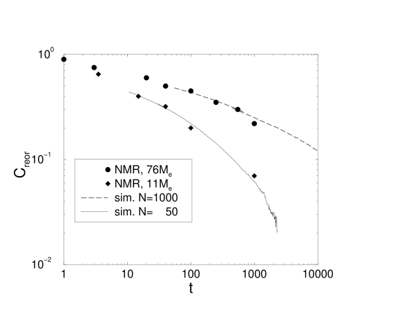
Figure 6: Comparison of $C_{reor}$ from our simulations ($l_{p}=5$) with the experiments on polybutadiene of ref. 6. Both are scaled to $C(0)=1$. The time axis for the simulation data is scaled empirically as an independent mapping to experimental times is not possible. The experimental times are measured in entanglement times which are derived from viscosity measurements.

The systems under study are not very long compared to the infinite chain limit as they are at most about 30 times the entanglement length (except for $N=1000,\,l_{p}=5$). Our exponents $\kappa$ come therefore closer to the $t^{-1/2}$ dependence. The system with persistence length $l_{p}=5$ is the most strongly entangled.[25] It is found to reorient slowest with an exponent between $0.25<\kappa<0.5$. The system with persistence length $l_{p}=1.4$ shows an algebraic decay faster than $t^{-1/2}$. This is probably because it is so weakly entangled, that the effects of entanglements are just starting to play a role. The exponents decrease systematically with persistence length, which, as discussed earlier, indicates an increasing degree of entanglement. The dependence on the degree of entanglement is supported by the very low exponent ($\kappa=0.29$) for a system with $l_{p}=5$ and chain length $N=1000$.

A $t^{-1/4}$ dependence of the correlation was found experimentally by Graf et al.[6] for a system with very long and therefore highly entangled PB chains (76 entanglement molecular weight $M_{e}$). They also observed a power-law with $t^{-1/2}$ for a system with a molecular weight of 11$M_{e}$. Figure 6 compares directly simulation (at $l_{p}=5$) and experiment; the ratio between the lengths in simulation and experiment is not exactly the same, it is, however, only important to be slightly or far above $M_{e}$. The agreement shows that the simulations reproduce well the exponents found in experiments. To achieve this agreement, the time axis of the simulated correlation functions has been rescaled empirically by 0.153 and 0.5 for $N=50\approx 8N_{e}$ and $N=1000\approx 160N_{e}$ respectively. This scaling may be used to infer a mapping to experimental times.

$l_{p}$	$\kappa$
1.4	$0.68$
3.0	$0.50$
5.0	$0.40$
5.0∗	$0.29$

Table 4: Algebraic fits ($t^{-\kappa}$) of the decay of double-quantum correlation functions $C_{DQ}$ for $N=200$ (see text and Figure 6).                                                                                                                 ^∗ The bottom line for $l_{p}=5$ has chain length $N=1000$ but the system is not equilibrated.

3.3 Interdependence of reorientation and translation of segments

If the reptation model holds the reorientation process is coupled to the translation of the polymer in its tube. A useful relation to monitor is, therefore, the reorientation correlation function of the chain tangent vector versus the mean-squared displacement of the monomers defining it, irrespective of the time. This relation has to be averaged over a finite time window $2t_{av}$, which is centered at some time $t_{m}$ and does not necessarily start at $t=0$.

$$C_{reor}(\Delta r^{2}) = \Big{\langle}P_{2}[\vec{u}(0)\vec{u}(t)]\Big{\rangle}_{t_{m}-t_{av},t_{m}+t_{av}}\;,$$ (10)

$$\Delta r^{2} = \Big{\langle}[\vec{r}(t)-\vec{r}(0)]^{2}\Big{\rangle}_{t_{m}-t_{av},t_{m}+t_{av}}\;,$$ (11)

Both $C_{reor}$ and $\Delta r^{2}$ depend parametrically on $t$. If, during $t$, the tube relaxes (reorients) then $C_{reor}$ is zero. Any deviation from zero indicates that the orientation is correlated over the time interval corresponding to the displacement. In our analysis we have ruled out possible artifacts from the translation of the system as a whole which could be present in Brownian dynamics.

In Figure 7a, it is seen that this function at short $t$ ($0<t<30000$) does not decay to zero, but shows a plateau, whose value depends on the stiffness: stiffer chains have a higher residual correlation. The presence of a plateau is a consequence of the finite length of the chain: Every finite polymer has a trivial residual static orientation correlation between distant chain segments in the direction of the end-to-end vector. If the motion of the chain is predominantly along the fixed tube, this residual correlation is also visible in the dynamic $C_{reor}(\Delta r^{2})$ shown here, since one chain segment samples the very same fixed tube at different times. We have seen in the preceding sections that stiffer chains have a higher reptation component in their dynamics. Hence, it is no surprise that they exhibit a larger residual correlation.

Figure 7b shows, for the most interesting case $l_{p}=5$, how the $C_{reor}(\Delta r^{2})$ depends on the position of the time window $t_{m}$. With increasing $t_{m}$, the reorientation correlation at $\Delta r=0$ goes to zero. At the same time, intensity moves to larger $\Delta r^{2}$, so that eventually a maximum at $\Delta r^{2}>0$ develops. This observation is explained by a scenario that includes, in addition to reptation, a diffusive or rather subdiffusive translation of entire chain segments through space, without significant reorientation of these segments: When a chain segment has reptated along the tube and comes back to its former part of the tube and hence its former orientation, it finds that this part of the tube itself has translated in the meantime. On the other hand, when it returns to its former absolute position ($\Delta r^{2}=0$) it is now in a completely different part of the tube and has a different orientation. This picture of short-scale transverse translation of stiff tube segments has been borne out by visualizations of individual chains.[25, 26]

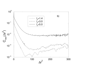
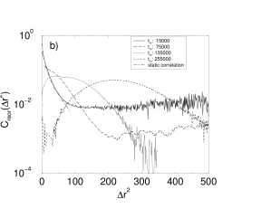
Figure 7: Reorientation correlation function depending on the mean-square displacement of monomers ($N=200$) a) Different systems at $0\leq t\leq 30000$. A running average was applied after the initial decay in order to show the possible plateau more clearly on all the curves in Figure a) and for the curve of $t_{m}=75000$ in Figure b) So the apparent final increase results from low statistics and is not meaningful. b) $l_{p}=5$ three different time intervals $t_{m}$ and comparison to static correlation. For reasons of statistics we always average over $2t_{av}=30000$, i.e. $t_{m}=15000$ means $0\leq t_{m}\leq 30000$. The static case is measured against topological distance, because distance in real space is not appropriate as the chain can fold back which leads for packing reasons (Section 4) to perpendicular alignments.

The time dependence of the plateau value contains information about the stability of the initial neighborhood. It measures the “similarity” i.e. correlation of the neighborhoods at different points in time as the chain returns. The neighborhood changes with time on a much longer time scale.

These results support the presence of reptation in our systems, as the chains come back to their former surrounding which has undergone only small changes in the meantime. As this memory effect preserves information about orientations, a tube picture is a suitable concept. However, the chains do not behave simply as the standard reptation picture would suggest. The reptation is considerably modified by their stiffness. Stiffer chains reptate in a more pronounced way, i.e. they follow the primitive path of the tube more closely as the stiffness suppresses the transversal motions efficiently. This leads to a higher degree of orientation memory for chains of the same length (Figure 7a).

4 Connection to Structure

The preceding section has shown that both the stiffness $l_{p}$ and the length $N$ have an effect on the dynamics of polymers already on the local level. In this section, we briefly review earlier results[21] about the local structure in polymer melts and how it is influenced by the chain architecture. This is done not only for comparisons within the model system. NMR experiments on melts have so far only been able to study the local dynamics. Any information on the structure had to be deduced from the dynamics using models. In contrast, the simulations of this work can be analyzed independently for both structure and dynamics. We, therefore, have an example case for which the assumptions can be checked that are used to analyze NMR experiments.

Of particular interest has been the question whether or not neighboring polymer chains are in any way aligned.[30] We therefore concentrate here on the static orientation correlation function $OCF$

$$OCF(r)=\Big{\langle}P_{2}[\vec{u}_{1}\vec{u}_{2}](r)\Big{\rangle}\;.$$ (12)

This function measures the mutual orientation of tangent vectors (defined in Eq. 6) of segments belonging to two different chains 1 and 2 as a function of their distance $r$. The second Legendre polynomial is used again, this time because our polymer chains have no direction, i.e. head and tail are equivalent. The $OCF$ is 1 for parallel orientation, $-1/2$ for perpendicular orientation, and 0 for random orientation.

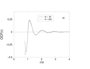
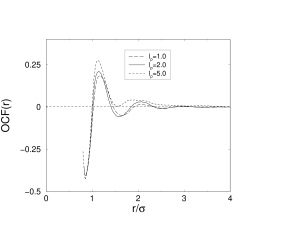
Figure 8: Comparison of the static orientation correlation of a) chains of different lengths (fully flexible system, $l_{p}=1$) and b) chains of different stiffness ($N=50$)

Figure 9: Comparison of the static orientation correlation of simple bead-spring chains against orientation correlation function of dimers on a perturbed fcc lattice, the dotted line is a spline curve as a guide to the eye.

The detailed discussion of the various $OCF$s is given elsewhere.[15, 21] Here we only note that the $OCF$ is a strictly local property. The chain length $N$ has no influence whatsoever on the short-range mutual orientation of two chains, even if one $N$ is below the entanglement length $N_{e}\approx 32$ and the other above (Figure 8a). The influence of the stiffness $l_{p}$ on the structure is clearly visible (Figure 8b), but small. We may conclude that the two parameters $N$ and $l_{p}$, which both influence significantly the local reorientation dynamics, have little ($l_{p}$) or no ($N$) effect on the local packing of chains. The fact that the chain length is not important for the local structure means that entanglements cannot be important either. This is yet another manifestation of the entanglement length $N_{e}$ being a purely dynamical quantity.

Local packing is, however, strongly influenced by another local quantity (which, in contrast, contributes little to the dynamics [31]), namely the excluded volume of the monomers. An example of this is shown in Figure 9. Here, the $OCF$ for a flexible chain ($l_{p}=1,\,N=50$) is overlaid by the $OCF$ for dimers on a randomly perturbed lattice. The monomers occupy fcc lattice sites whose positions were randomly displaced by small amounts to emulate finite temperature. The $OCF$ was then evaluated between all possible pairs of dimers which do not share a common atom. Although the $OCF$ for the dimers is much more accentuated than for the amorphous melt one can clearly see the short-range orientation of dimers shining through in the $OCF$ of the melt.

One may, therefore, conclude that local structure and local dynamics in polymer melts are dominated by different properties of the polymer. For this reason, it may be difficult to infer one from experimental results on the other.[31]

5 Conclusions

The reorientation of short segments in polymer chains in dense melts is governed by two subsequent processes. The fast one leads to an algebraic decay of the reorientation correlation function and the slow one to an exponential decay. The correlation times of both depend on the chain length as well as on the chain stiffness. Increasing chain stiffness leads to a strong slowing of the reorientation on both time scales.

A qualitative comparison of our reorientation correlation function showed that the power laws of the reorientation correlation function measured in double-quantum NMR experiments of systems not too far above the entanglement molecular weight could be reproduced. Therefore, our simplistic model, which is probably the simplest possible to incorporate stiffness and excluded volume, successfully describes the qualitative features of the dynamics. With our results, thus validated against experimental data, the reorientation correlation functions $C_{reor}(t)$ can be regarded as meaningful. In contrast, our simple model cannot explain two other experimental observations. The initial plateau of $C_{reor}(t)$, the so-called dynamical order parameter[6], of the experiment is not found, and in experiment the difference between persistence length and entanglement length is larger. Detailed atomistic models are probably necessary, in order to capture these features [26, 31].

One main result of this investigation is that, for the local reorientation to relax slowly, the chains have to be both stiff and long. Local stiffness ensures that the memory of orientation is not already lost during the fast algebraic process. On the other hand, the chains have to be above the entanglement length for the slow exponential process to extend into the experimentally observable regime (milliseconds in NMR). Although in principle both processes are always present, they have to span a big enough range in intensity and time, in order to be detectable in experiments. In agreement with our results, it has been found previously that the chain length has only little influence on the local reorientation, as long as it is below the entanglement length. In united atom polyethylene below the entanglement length local orientation relaxes like a stretched exponential, whereas the relaxation of the end-to-end vector is well described by the Rouse model.[19]

Although the dynamic reorientation correlation functions are found to be in qualitative agreement with experiments and theoretical predictions, our work shows that this does not necessarily imply an increase of static order due to topological entanglements of the polymer chains. The static local order increases with chain stiffness but does not at all depend on chain length. The entanglement length has emerged as a central quantity to explain the dynamics of flexible and especially stiff chains. It is not easily determined uniquely as there are several different definitions which lead to different values. This difficulty becomes even worse for chains with intrinsic stiffness. Nonetheless, we can say that the entanglement length in any definition decreases dramatically as the persistence length is increased. Evidence for this is found in the chain length dependence of the center of mass diffusion coefficient and in the segment size governing the long time relaxation of local order. In the system with $l_{p}=5$, it is questionable whether any length scale can be described by Rouse dynamics. The very local scales up to the persistence are dominated by bending modes and the very big length scales are dominated by entanglements. As $N_{e}l_{b}$ approaches $l_{p}$, the Rouse regime disappears between these two extremes.

A renormalization of the local scale properties onto an effective monomer or Kuhn segment is possible for static structural aspects as there is only one relevant length scale, namely the persistence length. However, this renormalization fails for dynamical properties of stiff polymers because two length scales (and the associated time scales) interdepend.[25] In dynamics one encounters, in addition to the persistence length, the entanglement length which describes the topological constraints imposed by non-crossability of the chains. When the two scales come into the same order of magnitude, new behaviors emerge which can not be deduced by renormalizing to Rouse dynamics or other simple models. The fact that the dynamics is not described appropriately by analytical theories implies also that the connection of translational and rotational dynamics is not a priori known. This has to be kept in mind by interpreting NMR experiments which predominantly measure reorientation.

The concept of reptation is supported by the existence of a time-dependent plateau value of reorientation as a function of the length of the diffused path in our simulations. Reptation is more pronounced if the chains are stiffer because of both the intrinsic stiffness and the stronger entanglement. They lead to the chain being more closely confined to the primitive path of the tube.

An analysis of the dependence of $N_{e}$ on $l_{p}$ and further consequences for chain and monomer motions will be discussed in more detail elsewhere.[25]

Appendix A List of Symbols

$\alpha$	strength of FENE potential
$\vec{B}$	magnetic field axis
$b$	strength of bending potential
$\beta$	amplitude of reorientation correlation function
$C_{DQ}$	double quantum correlation function
$C_{reor}$	reorientation correlation function
$D$	center-of-mass diffusion constant
$d$	chain segment length
$\epsilon$	nonbonded interaction strength
$k_{B}$	Boltzmann’s constant
$\kappa$	decay exponent for correlation function
$l$	distance along chain contour
$l_{b}$	bond length
$l_{p}$	persistence length
$l_{K}$	Kuhn segment length
$m$	monomer mass
$M_{e}$	entanglement molecular weight
$N$	chain length in monomers
$N_{C}$	number of chains

$N_{e}$	entanglement monomer number
$OCF$	orientation correlation function
$P_{2}$	second Legendre polynomial
$R$	characteristic length of FENE potential
$R_{end-end}$	end-to-end distance
$R_{gyr}$	gyration radius
$r$	distance
$\vec{r}$	position vector
$\rho$	density
$S$	dynamical order parameter
$\sigma$	monomer diameter
$T$	temperature
$T_{1}$	spin-lattice relaxation time
$t$	time
$t^{*}$	time unit
$t_{a}v$	averaging time
$t_{m}$	point of time for correlation of orientation and translation
$t_{sim}$	simulation time
$\tau_{e}$	entanglement time
$\tau_{R}$	Rouse time
$\tau_{reor}$	reorientation correlation time
$\vec{u}$	tangent unit vector
$\vec{u}_{d}$	tangent unit vector for segment length $d$
$V$	interaction potential

References

- [1] Schmidt-Rohr, K.; Spiess, H. W.; Multidimensional solid state NMR and polymers; Academic Press; New York; 1994.
- [2] Rouse, P. E.; J. Chem. Phys. 1953; 21, 1272–1280.
- [3] de Gennes, P.-G.; J. Chem. Phys. 1971; 55, 572–579.
- [4] Doi, M.; Edwards, S. F.; The Theory of Polymer Dynamics; vol. 73 of International Series of Monographs on Physics; Clarendon Press; Oxford; 1986.
- [5] Callaghan, P. T.; Samulski, E. T.; Macromolecules 1998; 31, 3693–3705.
- [6] Graf, R.; Heuer, A.; Spiess, H.; Phys. Rev. Letters 1998; 80, 5738–5741.
- [7] Müller-Plathe, F.; Schmitz, H.; Faller, R.; Prog. Theor. Phys. (Kyoto) Supplements, to appear in Vol. 138.
- [8] Dünweg, B.; Kremer, K.; Phys. Rev. Letters 1991; 66, 2996–2999.
- [9] Dünweg, B.; Kremer, K.; J. Chem. Phys. 1993; 99, 6983–6997.
- [10] Kremer, K.; Grest, G. S.; Carmesin, I.; Phys. Rev. Letters 1988; 61, 566–569.
- [11] Rigby, D.; Roe, R.-J.; J. Chem. Phys. 1988; 89, 5280–5290.
- [12] Kremer, K.; Grest, G. S.; J. Chem. Phys. 1990; 92, 5057–5086.
- [13] Takeuchi, H.; Roe, R.-J.; J. Chem. Phys. 1991; 94, 7446–7457.
- [14] Dünweg, B.; Grest, G. S.; Kremer, K.; in Whittington, S. G., ed., Numerical Methods for Polymeric Systems; vol. 102 of IMA Volumes in Mathematics and its Applications. Springer; 1998; 1998 pp. 159–196.
- [15] Faller, R.; Pütz, M.; Müller-Plathe, F.; Int J. Mod. Phys. C 1999; 10, 355–360.
- [16] Pütz, M.; Kremer, K.; Grest, G. S.; Europhysics letters 2000; 49, 735–741.
- [17] Moe, N. E.; Ediger, M. D.; Macromolecules 1995; 28, 2329–2338.
- [18] Paul, W.; Yoon, D. Y.; Smith, G. D.; J. Chem. Phys. 1995; 103, 1702–1709.
- [19] Harmandaris, V. A.; Mavrantzas, V. G.; Theodorou, D. N.; Macromolecules 1998; 31, 7934–7943.
- [20] Müller-Plathe, F.; J. Membr. Sci. 1998; 141, 147–154.
- [21] Faller, R.; Kolb, A.; Müller-Plathe, F.; Phys. Chem. Chem. Phys. 1999; 1, 2071–2076.
- [22] Weeks, J. D.; Chandler, D.; Andersen, H.; J. Chem. Phys. 1971; 54, 5237–5247.
- [23] Pütz, M.; Kolb, A.; Comput. Phys. Commun. 1998; 113, 145–167.
- [24] Kolb, A.; Molekular-Dynamik-Untersuchungen zum Wechselspiel zwischen flüssigkristalliner Ordnung und den Konformationen von Polymerketten; PhD thesis; MPI für Polymerforschung and Universität Mainz; 1999.
- [25] Faller, R.; submitted to Phys. Rev. Letters.
- [26] Faller, R.; Influence of Chain Stiffness on Structure and Dynamics of Polymers in the Melt; PhD thesis; MPI für Polymerforschung and Universität Mainz; 2000.
- [27] McQuarrie, D. A.; Statistical Mechanics; Harper’s Chemistry Series; Harper Collins Publishers; New York; 1976.
- [28] Graf, R.; Hochauflösende Doppelquanten-NMR-Spektroskopie an amorphen Polymeren; Ph.D. thesis; MPI für Polymerforschung and Universität Mainz; Shaker Verlag, Aachen; 1998.
- [29] Ball, R. C.; Callaghan, P. T.; Samulski, E. T.; J. Chem. Phys. 1997; 106, 7352–7361.
- [30] Kolinski, A.; Skolnick, J.; Yaris, R.; Macromolecules 1986; 19, 2550–2560.
- [31] Faller, R.; et. al.; in preparation