Self Consistent Field Theory of Twist Grain Boundaries in Block Copolymers

Abstract

We apply self consistent field theory to twist grain boundaries of block copolymer melts. The distribution of monomers throughout the grain boundary is obtained as well as the grain boundary free energy per unit area as a function of twist angle. We define an intermaterial dividing surface in order to compare it with minimal surfaces which have been proposed. Our calculation shows that the dividing surface is not a minimal one, but the linear stack of dislocations seems to be a better representation of it for most angles than is Scherck’s first surface.

1 Introduction

Bulk equilibrium properties of diblock copolymer melts are relatively well understood[1]. Incompatibility of the monomers comprising the two blocks drives the system toward ordered structures in which the number of contacts between dissimilar monomers is reduced, subject to various constraints. These ordered phases, of which the simplest is lamellar, are thermodynamically stable below some order-disorder transition temperature.

When the system is taken below this temperature, the lamellar phase is nucleated typically in distinct grains which differ, one from the other, by the orientation of the lamellae within them. The interface between lamellae of different grains constitutes a grain boundary, which can be considered an equilibrium structure arising from a constraint that imposes the different orientations of the lamellae of the two grains.

Because the lamellae of block copolymers lack any internal order, their grain boundaries are simpler than those between grains of crystalline solids. While the latter are combinations of five different independent boundaries, the former can be decomposed into only two independent ones. In the kink grain boundary, the normals perpendicular to the lamellae of the two grains define a plane which is perpendicular to the plane of the boundary. Kink grain boundaries have been studied recently both experimentally [2, 3, 4] and theoretically [5, 6, 7]. In the twist grain boundary (TGB), the plane defined by the normals is parallel to the plane of the boundary. The angle, $\alpha$, between the normals defines the twist angle. The geometry is shown in Fig. 1 where we fix the convention we use throughout: $x$ is the direction perpendicular to the grain boundary and $y$ and $z$ are in the plane of it; normals to the lamellae of the two grains are at angles $\pm\alpha/2$ with respect to the $y$ axis. Twist grain boundaries have been the subject of a thorough experimental study[8], but have received less theoretical attention.

Figure 1: Schematic of a twist grain boundary in which one looks down the $x$ axis. As $x\rightarrow\infty$, the IMDS approach that of the lamellar bulk, shown in dashed lines, while as $x\rightarrow-\infty$, the IMDS approach that of the lamellar bulk shown in solid lines. Normals to the planes of the bulk lamellae make angles of $\pm\alpha/2$ with respect to the $y$ axis.

Two different kinds of twist grain boundaries have been observed. The simplest consists of a stack of planes. In each plane, the orientation of lamellae differs slightly from those in planes above and below it. The structure is periodic along the stacking direction. It is observed for small twist angles ($\alpha<15^{\circ}$) only. A heuristic model for this boundary was proposed by Gido et al. [8] and checked against their experimental data, with good results.

The other structure, observed for all angles, is quite different: it is doubly periodic. A surface which displays this double periodicity is Scherck’s first surface, one which is characterized by zero mean curvature everywhere. It is shown in Fig. 2 for a twist angle $\alpha=0.5$ radians. This minimal surface was first proposed as a model of the TGB by Thomas et al.[9]. The reasoning is as follows. Suppose that one can ignore the components of the system, the block copolymers and the constituent monomers, $A$ and $B$ of the two blocks, and focus instead on the internal interfaces which divide the $A$-rich lamellae from the $B$-rich ones. Suppose further that one can ignore the finite thickness of these internal interfaces and approximate them by a suitably defined surface, the intermaterial dividing surface, (IMDS). The area of this surface is extensive, i.e. proportional to the volume of the system. Under these assumptions, the bulk free energy of the system should be expressable as the energy of this surface. Minimization of this free energy leads to the surface with minimum area subject to the constraint that it separate regions of certain volume. This is a surface of constant mean curvature. In particular for a symmetric system in which the volumes are equal, and that is the case for a diblock with equal volumes of $A$ and $B$ monomers, the constant value of the mean curvature is zero. Such surfaces are called minimal surfaces. The choice of the appropriate minimal surface depends upon boundary conditions and expected symmetries. Scherck’s first surface[10] was chosen in Ref [8] for comparison with experimental results because it connects two sets of parallel planes, the normals of which form an angle $\alpha$. The explicit expression for the surface is quite simple:

$$\exp\left[\frac{2\pi}{D}x\sin\alpha\right]=\frac{\cos\left[\frac{2\pi}{D}\{\cos(\alpha/2)y+\sin(\alpha/2)z\}\right]}{\cos\left[\frac{2\pi}{D}\{\cos(\alpha/2)y-\sin(\alpha/2)z\}\right]},$$ (1)

The equation defining the surface pertains only in the regions for which the right hand side is positive. This condition defines a chessboard-like domain in the $y$-$z$ plane (as a consequence of which the surface is sometimes referred to as “Scherck’s doubly periodic surface”). Far from the grain boundary, whose center is at $x=0$, the nature of the surface is easily inferred from Eq. 1: when $x\to-\infty$ the r.h.s. must vanish, and this defines a set of parallel planes with unit normal $(0,\cos(\alpha/2),\sin(\alpha/2))$ and spacing $D/2$. The period of the IMDS is half that of the lamellar phase, $D$, hence our convention. Similarly, when $x\to\infty$ the r.h.s. must diverge, and this defines a set of parallel planes with unit normal $(0,\cos(\alpha/2),-\sin(\alpha/2))$ and spacing $D/2$.

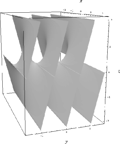
Figure 2: Scherck’s first surface is shown for a twist angle of $\alpha=0.5$ and a scale $D=1$.

A different description of the grain boundary, due to Renn and Lubensky [11], is that of a linear stack of dislocations (LSD). The model of a single dislocation is again a minimal surface, the helicoid. The whole structure arises from the stacking of infinitely many dislocations along a line. In this case the dislocations have vorticity along the $y$ axis with a pitch $D$, and are stacked along the $z$ axis with a separation $D/(2\sin(\alpha/2))$. It was later shown [12] that this approach is actually equivalent to the description employing Scherck’s surface, up to a $\cos(\alpha/2)$ dilation of the $x$ axis, the LSD being more “compressed” than Scherck’s surface.

The above approaches are valuable in providing simple models of the grain boundary which can be compared with experiment. They suffer, however, from the approximations which are inherent in the approach. Most importantly in the system of block copolymers, they ignore the physical constraints of incompressibility which causes the chains to stretch in order to fill the available volume. As a consequence, the IMDS is not a surface of constant mean curvature, a point made compellingly by Matsen and Bates[13], and confirmed in experiment[14].

Therefore we have studied the twist grain boundary in block copolymer systems using the self-consistent field theory in Fourier space which has been successful in describing lyotropic phases of block copolymer melts[15]. We follow the approach of Matsen[6] who adapted it to kink grain boundaries. First we will introduce the particular implementation of the theory which is useful in this case. We then present results for the TGB obtained within this framework and compare them with Scherck’s first surface and the LSD. We conclude with a brief discussion.

2 Theory

We consider an incompressible melt of $n$ AB diblock copolymers each composed of $N$ segments of volume $1/\rho_{0}$; the volume of the system is $V=nN/\rho_{0}$. The polymers are modeled as Gaussian random walks with statistical step length $a$. The natural length scale of the problem is the end to end mean distance, $aN^{1/2}$. To describe the incompatibility between A and B monomers the standard Flory-Huggins parameter, $\chi$, is introduced; the product $\chi N$ sets the units of energy and temperature.

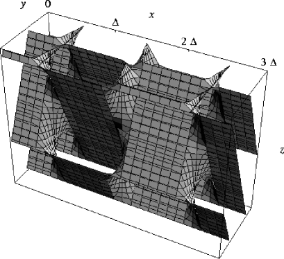
Figure 3: Schematic of the system, periodic in all three directions, on which we perform our calculations. The original system of interest is recovered on letting $\Delta$ increase without limit.

We utilize the SCFT method expressed in Fourier space as in Ref. [15], a method suited to the study of periodic phases. A system containing a twist grain boundary, however, is only periodic in the coordinates $y$ and $z$, but not in $x$. In order to circumvent this difficulty, we adopt the same strategy employed by Matsen in his study of the kink grain boundary[6]: to express the desired system as one periodic in all three directions in the limit in which one period becomes infinite. We therefore consider the system shown in Fig. 3 which, in addition to being periodic in $y$ and $z$ is periodic in $x$ with period $\Delta.$ We impose a reflection symmetry around $x=\Delta/2$, i.e., $(x,y)\to(\Delta-x,y)$. The desired grain boundary free energy per unit area, $\Gamma$, of the original system is obtained from the free energy, $F(\Delta)$, of our system according to

$$\Gamma=\lim_{\Delta\to\infty}[F(\Delta)-F_{\mathrm{b}}]\frac{\Delta}{V},$$ (2)

where the bulk free energy $F_{\mathrm{b}}=\lim_{\Delta\to\infty}F(\Delta)$, and the area of the grain boundary is $V/\Delta$. As the natural unit of area per polymer is $V/naN^{1/2}$, the natural unit of the grain boundary free energy is $k_{\mathrm{B}}TnaN^{1/2}/V$. Thus the boundary free energy can be written

$$\gamma\equiv\frac{V}{k_{\mathrm{B}}TnaN^{1/2}}\Gamma=\lim_{\Delta\to\infty}\frac{F(\Delta)-F_{\mathrm{b}}}{k_{\mathrm{B}}Tn}\frac{\Delta}{aN^{1/2}}$$ (3)

As the system is now periodic in all directions, we can expand all functions of position into a complete, orthonormal, set of eigenfunctions, $f_{lmn}$, of the Laplacian operator[15], eigenfunctions which explicitly express the symmetries of the system. It is clear that it is invariant under a rotation of $\pi$ about the $x$ axis, i.e. under $(x,y,z)\to(x,-y,-z)$. It is also invariant under rotations of $\pi$ about the $y$ and $z$ axes as well. Therefore the system is invariant with respect to the change in sign of any two of the coordinates. These considerations, together with the imposed reflection symmetry around $x=\Delta/2$, lead to the choice of functions

$$\begin{array}[]{l}f_{lmn}(x,y,z)=\\ =\left\{\begin{array}[]{l}c_{l}c_{m}c_{n}\cos(lk_{x}x)\cos(mk_{y}y)\cos(nk_{z}z),\\ \qquad\qquad\textrm{if $l$ is even}\\ c_{l}c_{m}c_{n}\sin(lk_{x}x)\sin(mk_{y}y)\sin(nk_{z}z),\\ \qquad\qquad\textrm{if $l$ is odd},\\ \end{array}\right.\end{array}$$ (4)

where $k_{x}=\pi/\Delta$, $k_{y}=2\pi\cos(\alpha/2)/D$ and $k_{z}=2\pi\sin(\alpha/2)/D$. Again $D$ is the bulk lamellar period.

It should be clear from Fig. 1 that the natural coordinates in which to express the periodicity of the system are $(y/D)\cos(\alpha/2)\pm(z/D)\sin(\alpha/2)$. Indeed Scherck’s surface, Eq. 1, is expressed in them. Translating an expansion in those coordinates into an expansion in $x$, $y$, and $z$, one sees that the parity of $m$ and $n$ above must be the same. Finally the $c_{l}$ are determined by orthonormality:

$$\frac{1}{V}\int f_{lmn}(\mathbf{r})f_{l^{\prime}m^{\prime}n^{\prime}}(\mathbf{r})d\mathbf{r}=\delta_{ll^{\prime}}\delta_{mm^{\prime}}\delta_{nn^{\prime}}.$$ (5)

Thus $c_{0}=1$ and $c_{i}=\sqrt{2}$ for $i>0$. This completes the specification of the basis functions.

One might think it necessary to impose an additional invariance: that the calculated free energy of the grain boundary with twist angle $\alpha\leq\pi/2$ be identical to that with angle $\pi-\alpha$ because, after an interchange of $y$ and $z$, the one boundary is identical to the other. However the grain boundary free energy we calculate already displays the symmetry $\Gamma(\alpha)=\Gamma(\pi-\alpha)$ without further restriction of the basis functions. This can be seen from the fact that under $\alpha\rightarrow\pi-\alpha$, the wavevector components $k_{y}$ and $k_{z}$ interchange. Thus an interchange of the coordinates $y$ and $z$ and a relabelling of the dummy indices $m$ and $n$ suffices to make the expressions for the free energies of the two grain boundaries identical.

We expand all functions of position in terms of the above basis functions. Of course the infinite set must be truncated in a numerical calculation, and our computer resources impose a maximum slightly below $400$ functions. The results presented below are obtained for the choice of $5$ values for $m$, $5$ for $n$ and $15$ for $l$ as the results are more sensitive to the number of components in the $x$ direction than in $y$ or $z$. To be consistent with this choice, we take the corresponding bulk lamellar phase to be that obtained from $5$ Fourier components.

We have chosen $\chi N=15$, an intermediate value for which an intermaterial dividing surface is well delineated, but not so sharp as to require a large number of basis functions to describe. A value of $\Delta\sim 5aN^{1/2}$ is sufficient typically for the free energy to become insensitive to further increases in this parameter. With our 375 basis functions, our results for the free energy at $\alpha=\pi/2$ are accurate to within 1%. Larger values of $\chi N$ would require additional basis functions. Smaller values of $\chi N$, nearer the order disorder transition temperature of $\chi N=10.49$, cause periodic modulations of the dividing surface to appear which extend away from the grain boundary. This behavior, similar to that reported for the kink grain boundary [5, 6], is likely to be strongly modified by fluctuation effects which are absent in the SCFT.

3 Results

In Fig. 4 we show results for the twist angle $\alpha=0.4\approx 22.9^{\circ}$. We have plotted, for several values of $x$, contours of constant order parameter, the difference between the volume fractions of the two monomers. In these gray scale plots, the maximum absolute value of the order parameter is $0.88$. Fig. 4(a) shows a slice at infinitely large $x$, that is, a cross section through the bulk system. Figs. 4(b) and (c) show slices at the values of $x=0.2\ aN^{1/2}$, and $0$, that is, at the grain boundary itself.

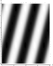
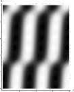
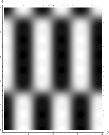
Figure 4: Slices through the grain boundary showing the monomer distribution at different distances: (a) In the limit of $x\rightarrow\infty$, i.e. the bulk, (b) $x=0.2aN^{1/2}$, (c) $x=0$, i.e. at the grain boundary itself. In these gray scale plots, the maximum absolute value of the order parameter is $0.88$.

We would like to compare the distribution of monomers obtained in our solution with Scherck’s first surface, which is a model for the intermaterial dividing surface. One way to do this is to calculate within our solution the value of the order parameter, $\delta\phi(\mathbf{r})\equiv\phi_{A}(\mathbf{r})-1/2$, at the points $\mathbf{r}_{\mathrm{S}}$ defined by Scherk’s surface. The value of $\delta\phi(\mathbf{r}_{\mathrm{S}})$ vanishes as $x\rightarrow\pm\infty$ because Scherck’s surface and the intermaterial dividing surface of our solution, defined by $\delta\phi(\mathbf{r}_{\mathrm{I}})=0$, coincide in that limit. A convenient measure of the similarity of the two dividing surfaces, therefore, can be defined by computing

$$I_{\mathrm{S}}\equiv\int\ d\mathbf{r}\left[\phi_{A}(\mathbf{r})-1/2\right]^{2}\delta(\mathbf{r}-\mathbf{r}_{\mathrm{S}})$$

A measure $I_{\mathrm{LSD}}$ for the LSD can be defined in the same manner.

A second means to compare the surfaces is to calculate the volume of the region which is enclosed between the two surfaces to be compared. This is easy to implement by a Monte Carlo integration technique in which points of the unit cell are taken at random and checked to determine whether the two surfaces agree, or not, in the assignment of the point to the A-rich region. The relevant quantity is $(\delta V)\Delta/VN^{1/2}a$, the fraction of the volume $\delta V$ for which there is disagreement, normalized by the area of the grain boundary $V/\Delta$. The factor $N^{1/2}a$ ensures that this measure, which we denote $I^{\prime}_{\mathrm{S}}$, is dimensionless.

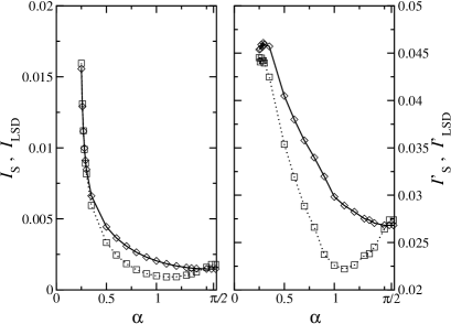
Figure 5: Measures of the similarity between the intermaterial dividing surface defined by our calculation and that of Scherck’s first surface (diamonds, joined by solid line) and that defined by the linear stack of dislocations (squares, dotted line). Except near twist angles of $\pi/2$, the latter is a better representation.

These two measures are plotted in Fig. 5. They indicate that the LSD is a better representation of the intermaterial dividing surface over almost the entire range of twist angles except, perhaps, quite close to $\pi/2$. As the angle decreases, both measures tend to the same limit, of course. (Recall the only difference between the two surfaces is a dilation of $\cos(\alpha/2)$.)

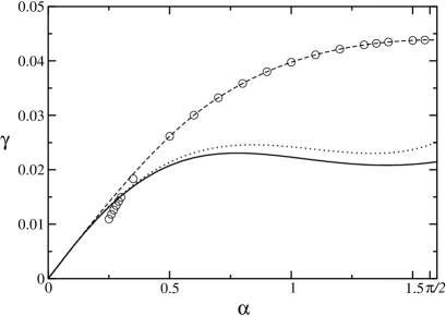
Figure 6: Free energy per unit area, $\gamma$, of the twist grain boundary as a function of twist angle $\alpha$. The circles show our results, the dashed line is a fit to them (extrapolated to $\alpha=0$) taking into account only data for $\alpha>0.5.$ Also shown are the approximate free energies we have calculated from the expressions in Ref. [12] for Scherck’s first surface (solid line) and the linear array of dislocations (dotted line) which include only bending and compression energies.

The grain boundary free energy as a function of the twist angle is shown in Fig. 6. The circles show the results of our calculation. For values of the twist angle greater than $0.5$ radians, our results are accurate to within $5\%$, improving towards $1\%$ as they approach $\pi/2$. The dashed line has been drawn through these values and extrapolated to zero. We have also included several other points for smaller values of $\alpha$. The number of basis functions employed is insufficient for the grain boundary free energy to have converged to within $5\%$. Nevertheless, we have included them as they appear to indicate that the behavior of the free energy as the angle approaches zero may not be linear, the behavior expected if, at very low densities, dislocations repel one another[12]. It has been argued, however, that at very low densities, dislocations attract one another[16].

One notes that the grain boundary free energies are rather small: that of the grain boundary with twist angle of $\pi/2$ is, at the same incompatibility, $\chi N$, somewhat less than half the energy of the boundary with tilt angle of $\pi/2$[6]. Perhaps this should not be too surprising. In the approximation noted earlier of treating the intermaterial dividing surface as a surface of constant mean curvature, with an energy given by the Helfrich free energy[17], the grain boundary free energy would be identically zero[18].

The free energy of a system with a twist grain boundary was calculated previously by Gido and Thomas[19]. They applied a version of the self consistent field to a brush of infinitely stretched chains anchored to a given saddle-shaped surface, and also carried out an independent calculation based on work of Wang and Safran[17]. However they report their results in terms of the extensive free energy per chain in the region of Scherck’s surface. This is not a uniquely defined quantity, nor is it the thermodynamic grain boundary free energy per unit area which we have calculated, so direct comparisons are precluded.

We have chosen to compare our results with those of Kamien and Lubensky[12]. We emphasize that the two calculations are rather different in principle. In the approach we have employed, the free energy of the block copolymer system is calculated directly, assuming nothing other than the applicability of self consistent field theory. In particular, we do not employ elasticity theory, or assume that displacements from a reference system without a grain boundary are small, etc. In contrast, that of Ref. [12] assumes that the bulk system can be adequately described as a series of surfaces, and the energy of this system of surfaces can be expanded assuming small displacements. A further difficulty which arises when applying the calculation of Ref. [12] to a block copolymer system is that the volumes on either side of the surfaces are undifferentiated, whereas in the block copolymer system, these volumes are filled with different monomers. Thus the symmetry of the system considered by Kamien and Lubensky is not the same as that of ours. As a consequence, there are more elastic constants in an elastic description of a block copolymer lamellar phase than the two utilized by them in their description of liquid crystalline smectics[20].

Having acknowledged these caveats, we calculate the bending and compression contributions to the free energies of Scherck’s first surface and of an LSD surface as given in Ref. [12]. As noted in the Introduction, a number of parameters needed to evaluate these free energies are unknown, being inputs to the phenomenological theory. However we can provide some of these values from our work. Thus we calculate the lamellar spacing to be $D=1.5155\ aN^{1/2}$, and the dimensionless compression modulus to be $B=3.01$. The dimensionless bending modulus is unknown but can be estimated [21] to be $\kappa\approx 0.115$. The only unknown which remains is the size of the “core region”, which provides a cutoff to the otherwise divergent integrals for the compression free energy estimated in [12]. This can be estimated from the slope of the dotted line in Fig. 6. We obtain, thereby, a value of $\approx 0.191aN^{1/2}$, i.e., $25\%$ of the IMDS spacing $D/2$. Of course, there is no reason that this core region should not depend on $\alpha$, but were we to obtain the size of the core from our data at each value of the twist angle, the result would simply be a mapping of the results of Ref. [12] to ours, and no independent comparison would be possible. Using these parameters, we have evaluated the free energy given in Ref. [12] of the appropriate Scherck’s surface and of the linear superposition of dislocations. These are shown in Fig. 6 as solid and dotted lines respectively. The LSD has a free energy closer to our result than does Scherck’s surface, just as it is closer to our intermaterial dividing surface. Both approximations underestimate the grain boundary free energy of the block copolymer system by a factor which increases with twist angle, and is about two at $\alpha=\pi/2$.

4 Conclusions and outlook

We have applied self consistent field theory to twist grain boundaries in block copolymer melts. Our calculation is more direct than earlier ones and provides greater information concerning the monomer densities throughout the volume. It also expresses the grain boundary free energy in terms of the directly measurable volume per chain and radius of gyration as opposed to elastic modulii of internal interfaces. The boundary free energy was obtained as a function of twist angle, and found to be quite small; smaller than kink grain boundaries of the same angle and incompatibility.

We have compared our results to previous phenomenological calculations to show that the intermaterial dividing surface is not given by either surface, Scherck’s first surface or the linear stack of dislocations, but that of the two, the latter is a better representation over most twist angles except near $\pi/2$.

We comment briefly on the other type of twist grain boundary which has been observed at small twist angles[8] , the one consisting on a stack of lamellae which are twisted slightly and remain continuous. We have not investigated it is because we failed to find an appropriate periodic boundary condition which does not contribute to the excess surface free energy. Although it is possible to calculate the contribution to the excess surface free energy of any choice of boundary condition and then to subtract it from the total excess, leaving the desired grain boundary free energy, the procedure is tedious. However simple examination of this boundary leads to the conclusion that the grain boundary free energy must be approximately twice that of a kink grain boundary. This is because the lamellae within the boundary and those far from it meet in what approximates a kink grain boundary. (Fig. 4 of Ref. [8] shows this nicely.) The free energy of a kink grain boundary grows as $\theta^{3}$ for small kink angle $\theta$[5, 6]. Of course we do not know the relation between the angle, $\theta$, of this “effective” kink grain boundary and the twist angle $\alpha$. Nonetheless, if we assume that the relation is linear, then the twist grain boundary energy would grow as $\alpha^{3}$ for small twist angles and would be favored over those we have modeled here, which would in fact be metastable but long-lived as their energy is small. This is in accord with the experimental result that both forms of boundary are observed at small twist angles. But at larger angles such grain boundaries would be disfavored compared to those considered in this paper. This is in accord with the fact that they are not seen experimentally.

References

- [1] I.W. Hamley The Physics of Block Copolymers (Oxford Univ. Press, Oxford, 1998).
- [2] S.P. Gido and E. L. Thomas, Macromolecules 27, 6137 (1994).
- [3] T. Hashimoto, S. Kuizumi, and H. Hasegawa, Macromolecules 27, 1562 (1994).
- [4] Y. Nishikawa, H. Kawada, H. Hasegawa, and T. Hashimoto, Acta Polymerica 44, 247 (1993).
- [5] R.R. Netz, D. Andelman, and M. Schick, Phys. Rev. Lett. 79, 1058 (1997).
- [6] M.W. Matsen, J. Chem. Phys. 107, 8110 (1997).
- [7] Y. Tsori, D. Andelman, and M. Schick, Phys. Rev. E 61, 2848 (2000).
- [8] S.P. Gido, J. Gunther, E.L. Thomas, and D. Hoffman, Macromolecules 26, 4506 (1993).
- [9] E.L. Thomas, D.M. Anderson, C.S. Henkee, and D. Hoffman, Nature 334, 334 (1988).
- [10] J.C.C. Nitsche, Lectures on Minimal Surfaces, transl. J.M. Feinberg, ed. A. Schmidt, (Cambridge University Press, New York, 1989)
- [11] S.R. Renn and T.C. Lubensky, Phys. Rev. A 38, 2132 (1988).
- [12] R.D. Kamien and T.C. Lubensky Phys. Rev. Lett. 82, 2892 (1999).
- [13] M.W. Matsen and F.S. Bates, J. Chem. Phys. 106, 2436 (1997).
- [14] H. Jinnai, Y. Nishikawa, R.J. Spontak, S.D. Smith, D.A. Agard, and T. Hashimoto, Phys. Rev. Lett. 84, 518 (2000).
- [15] M.W. Matsen and M. Schick, Phys. Rev. Lett. 72, 2660 (1994).
- [16] I.A. Luk yanchuk, cond-mat/9910350.
- [17] Z.-G. Wang and S.A. Safran, J. Chem. Phys. 94, 679 (1991).
- [18] We are indebted to Gerhard Gompper for reminding us of this.
- [19] S.P. Gido and E.L. Thomas, Macromolecules 27, 849 (1994).
- [20] L.D. Landau and E.M. Lifshitz, Theory of Elasticity, §10 (Pergamon, London, 1959).
- [21] Matsen [6] shows how can be determined from an analysis of the kink grain boundary at low angles. His analysis for yields . We could repeat his calculations for our value of , but as this modulus scales with the energy, we can approximate the modulus at our value of incompatibility by . Note that the same scaling of his result for the compression modulus at yields at , which is very close to the value of which we calculate directly.