Conductance peak motion due to a magnetic field in weakly coupled chaotic quantum dots

Abstract

We study the influence of moderate exchange interactions of electrons on the behavior of the peaks in the conductance of single electron transistors. We numerically reproduce recently observed features of both the peak positions and the peak heights magnetic field dependence. These features unambiguously identify the total spin $S$ of each ground state. We evaluate the probability of each $S$ (combination of spontaneous and induced magnetization) as a function of the exchange strength, $J$, and external magnetic field , $B$. The expressions involve only $J$ and $g$-factor as adjustable parameters. Moreover, in a surprisingly broad parameter range these probabilities are determined by certain linear combinations of $J$ and $B$.

In the Pauli picture, electrons populate the orbital states of a chaotic quantum dot or metallic grain in a sequence of spin up - spin down electrons. This means that the total spin of the system can be either zero (when the number of electrons $N$ is even) or one half (at odd $N$). It is well known, [1] that measuring the electron transport through a quantum dot one effectively studies its ground state (GS) properties. One can measure, e.g., the ohmic conductance by weakly connecting the dot with source and drain electrodes. This conductance can be studied as a function of the voltage, $V_{g}$, applied between the dot and a third electrode - gate. The energy of the system at a given number of electrons, $E_{N}$, is determined by the gate voltage, $V_{g}$. Each time when $E_{N}(V_{g})$ coincides with $E_{N+1}(V_{g})$ the conductance increases dramatically. Such a coincidence determines the position, $V_{g}^{(N)}$ of $N$-th peak in the conductance, which is proportional to $\mu_{N}$, determined as $\mu_{N}=E_{N}(0)-E_{N-1}(0)$. Accordingly, the distance between the peaks is $\propto\mu_{N}-\mu_{N-1}$. The height of the conductance peak is determined by the GS wave functions. Thus, studies of the conductance as function of $V_{g}$ allow to deduce properties of the manyparticle GS.

Recently, the behavior of the conductance peaks in metallic dots [2], carbon nanotubes [3], small chaotic GaAs [4] and Si [5] quantum dots was monitored as a function of $B$. In the following discussion we neglect the magnetic field coupling to the orbital degrees of freedom (For a 2D quantum dot one is allowed to do it when the magnetic field is inplane. For an ultrasmall dot this is a good approximation for a field in any direction, provided that it is small enough). In other words, we expect the field to manifest itself only through the Zeeman splitting - the field shifts the GS energy by $g\mu_{B}SB$, where $\mu_{B}$ is the Bohr magneton and $S$ denotes the GS total spin. For systems studied in Refs. [4, 5] the Zeeman splitting for $S=1/2$ becomes comparable to the mean single electron level spacing

$$\delta_{1}=<s_{i}>;\ \ \ s_{i}=\varepsilon_{i}-\varepsilon_{i+1},$$ (1)

(here $\varepsilon_{i}$ denotes the orbital energy of the one-electron orbital state $i$, and $<\ldots>$ stands for the averaging.) at $B\sim 1$ tesla for the GaAs [4] dot and $B\sim 10$ tesla for the Si dot [5]. Thus, up to a few Tesla $g\mu_{b}B\ll\delta_{1}$, i.e., in the Pauli picture the magnetic field only seldomly exceeds $s_{i}$ resulting in changes of the GS spin. As a result one should expect the following conductance peak behavior as function of the magnetic field (see Fig. 1a): (i) The peak positions ($\mu_{N}$) vary with $B$ as consecutive pairs creating an altering pattern of downward and upward moving peaks. The trajectories of the peaks are straight lines with the same slope of $g\mu_{b}/2$. (For the peak spacings ($\Delta_{N}$) the Pauli picture predicts a similar pattern with slopes of $g\mu_{b}$). Spin-orbit interactions may lead to fluctuations in the $g$ factor resulting in fluctuations in the slope magnitudes [6, 7], which will not change the pattern of downward and upward moving peaks. (ii) The peak heights are the same for each pair and change between neighboring pairs. (iii) Once $g\mu_{b}B$ exceeds a particular spacing $s_{i}$, the peaks should cross. The peak height is expected to switch at each crossing.

Experimental results confirm this picture for metallic dots and carbon nanotubes[2, 3], but contradict it for the semiconducting chaotic dots [4, 5]. In Fig. 1b we show the behavior of the conductance peaks as function of the magnetic field that follows from a model discussed later. Fig. 1b reproduces features of the semiconducting chaotic dot experiments (see e.g., Figs. 2 and 3 in Ref. [5]) much better than Fig. 1a. Peaks move as function of the magnetic field in bunches of two [4, 5] (peaks [3] and [4] in Fig. 1b) in the same direction and with the same slope. For these peaks the height does not come in pairs. Not every change in the direction of the motion of a peak looks like a crossing. For example, some of these changes are more abrupt - a particular example is peak [3]. Thus, a description of the system beyond the Pauli picture is needed.

FIG. 1.: Typical conductance dependence on the gate voltage and magnetic field, $B$, with and without exchange interaction: (a) $J=0$, (b) $J=0.1\delta_{1}$. $\mu^{\prime}_{N}$ is determined as $\mu^{\prime}_{N}=\mu_{N}-e^{2}/C$ and taken in arbitrary units. The vertical curves indicate the conductance while the circles indicate the peak maxima positions. The behavior of specific peaks (indicated by $[1]-[4]$) in (b) and the different regions of GS spin (depicted in the plot in units of $1/2$, i.e., $1$ corresponds to $S=1/2$, and separated for clarity by vertical lines) is discussed in the text.

This letter aims to explain the puzzling features of the magnetic field dependence of the conductance peaks positions and heights by spontaneous spin polarization of the electrons in the dot. The possibility of spontaneous magnetization has been in the center of much recent research [8, 9, 10, 11, 12, 13, 14]. It has been previously suggested as an explanation [9] to the puzzling absence of a bimodal distribution in the conductance peak spacings [15]. Such a magnetization was also predicted to lead to kinks in the parametric motion of the peaks, (e.g., due to orbital effects of a perpendicular magnetic field) [12]. Authors of a recent paper based on a random interaction model [13] note some deviations of the peak motion from the Pauli picture due to spontaneous magnetization.

The magnetization results from the exchange interaction between the electrons. In the presence of interaction the Pauli picture no longer holds. Indeed, it might be advantageous to lose in kinetic energy by placing electrons at higher orbitals in order to gain in the exchange energy.

A symmetric dot is spontaneously polarized every time there is a partially filled degenerate orbital - this is the familiar Hund’s rule in atomic physics. Accordingly, magnetization will occur in a chaotic dot once the orbitals are close enough to each other. Here we demonstrate that the exchange interaction explains the deviations from the Pauli picture listed above and also make definite predictions on the statistics of the peak motions which can be checked experimentally.

We use the following Hamiltonian to describe the electrons in a chaotic dot [14]:

$$H=\sum_{i}\varepsilon_{i}n_{i}+{{e^{2}N^{2}}\over{2C}}-JS(S+1)+g\mu_{b}SB.$$ (2)

The first term in Eq. (2) is the one-partical Hamiltonian, where $\varepsilon_{i}$ and $n_{i}$ are the energy of the i-th orbital and its occupation number. We assume that the energies $\varepsilon_{i}$ are characterized by the Random Matrix spectral statistics. Here we consider both orthogonal (GOE) and unitary (GUE) Dyson ensembles. The second term represents the charging energy. We ignore fluctuations in the capacitance $C$ [15] which are not important for the magnetic behavior. It was demonstrated in Ref. [14] for the most general form of the electron - electron interaction that the sample to sample and level to level fluctuations of the exchange interaction are negligible for systems with high Thouless conductance. This is the reason why the exchange energy can be presented in a simple form of the third term of Eq. (2) with some constant $J$ that does not fluctuate. (See Ref. [14] for the details.). Note that Refs. [10],[13] introduce different exchange terms.

We calculated the conductance using the energies $E_{N}$ and wave functions obtained numerically for GOE and GUE random matrix realizations. An example of the peak positions and heights evolution as functions of the magnetic field for a particular GOE realization is presented in Fig 1 for (a) $J=0$ and (b) $J=0.1\delta_{1}$. For both cases we present $\mu_{N}^{\prime}=\mu_{N}-e^{2}/C$.

It is not surprising that in Fig 1a one can see all the previously described features of the Pauli behavior. On the other hand, once even a weak exchange interaction is included the behavior changes qualitatively. For example, even in the vicinity of $B=0$, around a $S=1$ state (peaks [3] and [4] in Fig. 1b) the usual Pauli pattern is disrupted. Instead of an up and down moving pairs of identical peak height we see two down moving and then two up moving peaks with alternating height. The reason for this behavior is that first two consecutive orbitals are first filled with down spin electrons and only later they acquire up electrons. Generally the enhancement of the spin of the dot by $S$ will be accompanied by a $2S$ bunch of alternating height peaks moving with the same slope. If the peak spacing $\Delta_{N}$ is plotted, two sets of $2S-1$ flat curves sandwiching a sloped one will appear. Changes to the crossing patterns should be also attributed to the spontaneous magnetization. For example, such a case occurs when the spin of the GS between peaks $[3]$ and $[4]$ (indicated in Fig. 1b) switches from $S=1/2$ to $S=3/2$. Peaks $[3]$ and $[4]$ abruptly change their slopes and amplitudes (actually the amplitude vanishes due to spin blockade [16]). The amplitude of peak $[4]$ is equal to the amplitude of peaks $[1]$ and $[2]$ since the orbital, which occupation was documented by appearance of the $[1]$ and $[2]$ peaks, becomes once again available for tunneling through the combined effect of spontaneous and field-induced magnetization. Another change of slope and amplitude is seen once the GS between peaks $[2]$ and $[3]$ switches from $S=0$ to $S=1$. Thus, the exchange interaction can explain some of the qualitative behaviors seen in the experiment.

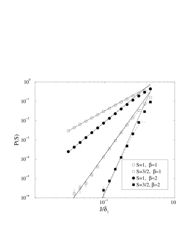
FIG. 2.: Probabilities $P_{J}(S)$ of $S=1$ and $S=3/2$ at $B=0$ as functions of the exchange strength $J$ for GOE ($\beta=1$) and GUE ($\beta=2$). The symbols represent numerical results, the solid curves correspond to the first order terms in Eq. (3) while the dashed lines involve the higher order corrections.

This model can also give quantitative predictions regarding the peak position movements. As illustrated above, the appearance of higher spin clearly manifests itself in these trajectories. Using Eq.(2) one can predict the frequency of spontaneous magnetization appearances. For weak exchange, $J\ll\delta_{1}$, the probability that the dot GS has a spin $S$ is determined by the probability of finding $2S$ orbitals so close to each other that the gain in exchange energy (due to the polarization) overwhelms the loss in the kinetic energy (due to single rather than double occupations of the orbitals).

Using methods described in details in[17] one can show that a sequence of $2S$ levels with a total energy smaller than $JS(S+1)$ which is necessary for the spin to reach the value $S$ at $J\ll\delta_{1}$ takes place with the probability:

$$P_{J}(S)=C_{S}^{\beta}\left({{J}\over{\delta_{1}}}\right)^{(\beta S+1)(2S-1)}\left(1-K_{S}^{\beta}{{J^{2}}\over{\delta_{1}^{2}}}\right).$$ (3)

Here $\lfloor R\rfloor$ denotes the integer part of a real number $R$ and, as usual, $\beta=1(2)$ corresponds to GOE (GUE). In Eq. (3) we took into account the main asymptotics of $P_{J}(S)$ at $J\to 0$ and the first order correction in $J^{2}/\delta_{1}^{2}$. The coefficients $C_{S}^{\beta}$ and $K_{S}^{\beta}$ depend on both $\beta$ and $S$. Their values for $S=1,3/2$ are presented in table I.

According to Eq.(3) the probability of a GS with a certain value of $S$ depends on $\beta$ and goes down rapidly as $S$ increases. In Fig. 2 we present the probabilities of $S=1$ and $S=3/2$ realizations as functions of the exchange strength, $J$, for the GOE ($\beta=1$) and GUE ($\beta=2$). The probabilities are obtained from a direct numerical solution of Eq. (2) (symbols) as well as from the analytical estimation, Eq. (3). One can see that for $J\leq 0.3$ both results coincide.

As already mentioned, one can unambiguouslydetermine the spin of each GS from the trajectories of the conductance peaks. This fact creates an opportunity to extract $J$ from the experimentally determined probabilities of different values of $S$. Note, that it is only one dimensionless parameter $J/\delta_{1}$ that controls the probabilities $P_{J}(S)$ of all spins at both possible values of $\beta$.

Magnetic field dependence of the probabilities of a given spin realization, $P_{J,B}(S)$, can be calculated in a similar way. It turns out that as long as the following linear combination of $J$ and $B$,

$$X={{J}\over{\delta_{1}}}+{{g\mu_{B}B}\over{\lfloor S+{{3}\over{2}}\rfloor\delta_{1}}},$$ (4)

remains small, the probabilities behave as

$$P_{J,B}(S)=C^{\beta}_{S}X^{(\beta S+1)(2S-1)}(1-K_{S}^{\beta}X^{2}),$$ (5)

In Fig. 3a the probabilities $P_{J,B}(S)$ for $S=1,3/2$ calculated numerically at $J/\delta_{1}=0.1$ are compared with the asymptotics of Eq. (5). The agreement turns out to be good as long as $g\mu_{B}BS<0.4\delta_{1}$.

The form of Eq. (5) and the higher order terms suggests that exchange interaction and Zeeman splitting enter the probabilities $P_{J,B}(S)$ only through the combination $X$. As can be seen from Fig. 3b, a general scaling

$$P_{J,B}(S)=F(S,X),$$ (6)

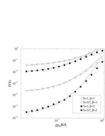
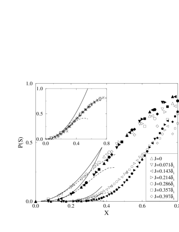
FIG. 3.: (a) Probabilities of $S=1,3/2$ for $J=0.1\delta_{1}$ as functions of the magnetic field $B$. The symbols represent numerical results, while the curves (solid - first order, dashed - second order) represent Eq. (5). (b) The same probabilities of measuring a spin value $S$ for different values of $B$ and $J$ scaled as functions of the parameter $X$, (Eq. (4)). Hollow symbols represent the GOE and filled symbols stand for the GUE. Large (small) symbols correspond to $S=1$ ($S=3/2$). One can clearly see that the scaling form holds much beyond the first couple of terms estimated here. Inset: probability of $S=1$, in a $\beta=1$ Hubbard model. The Hubbard model was solve using exact diagonalization (similar to Ref. [9]) for different lattices and fillings ($4\times 3$, $4\times 4$, $4\times 5$ with $4,6,8$ electrons ), and different values of on-site interactions, $U=0-2t$, and magnetic fields. The scaling parameter $X$ was calculated using $J(U)$ deduced from the spin dependence of the averaged energy. The $\times$ symbols correspond to the Hubbard numerical results, the $\bigtriangledown$ are the same as in (b). A full description of the Hubbard model results will be given elsewhere.

where $F(S,X)$ is some function of the scaling parameter $X$ and the spin $S$, holds for values of $X$ which much exceeds the range of validity of Eq. (5). Deviations from the scaling law Eq. (6) at higher $X$ are probably due to the fact that the probability to observe even higher spins ($S>3/2$) becomes already substantial. At $J$ close to $\delta_{1}$ one should use the approach of Ref.[14] to describe $P_{J,B}(S)$ analytically. It is important to stress that this scaling will hold for any system of interacting electrons as long as the Thouless energy is large and there is no spin orbit scattering. This is demonstrated in the inset of Fig 3b where results for a Hubbard model are presented.

In conclusion, we have shown that the presence of even a relatively weak exchange interaction explains many of the deviations from the Pauli picture seen in recent experiments [4, 5]. We calculate how the frequency at which different values of spin appear depends on weak exchange interaction and a moderate magnetic field. The strength of the exchange interaction, $J$, and the effective $g$-factor are the only adjustable parameters that determine the probabilities for a GS of the dot to have any given spin at any given magnetic field for both GOE and GUE cases. In particular we predict that these probabilities will follow a one parameter scaling law over a wide range of magnetic fields and exchange interaction strengths. To test these predictions experimentally one needs only enough statistics for the behavior of the conductance peaks.

The work at Princeton University was supported by ARO MURI DAAG55-98-1-0270. We are grateful to I. L. Aleiner, C. M. Marcus and L. P. Rokhinson for many useful discussions.

	$\beta=1$		$\beta=2$
	$S=1$	$S=3/2$	$S=1$	$S=3/2$
$C$	$\pi^{2}/3$	$9\pi^{4}/50$	$8\pi^{2}/9$	$81\pi^{6}/400$
$K$	$\pi^{2}/5$	$18\pi^{2}/49$	$8\pi^{2}/25$	$792\pi^{2}/1225$

TABLE I.: The factors $C_{S}^{\beta}$ and $K_{S}^{\beta}$ appearing in Eq. (3).

REFERENCES

- [1] M. A. Kastner, Rev. Mod. Phys. 64, 849 (1992); R. C. Ashoori, Nature 379, 413 (1996); P. L. McEuen, Science 278, 1729 (1997).
- [2] D. C. Ralph, C. T. Black and M. Tinkham, Phys. Rev. Lett.74, 3241 (1995).
- [3] D. H. Cobden et. al., Phys. Rev. Lett.81, 681 (1998).
- [4] C. M. Marcus (preprint)
- [5] L. P. Rokhinson, et. al., cond-mat/0005262.
- [6] K. A. Matveev, L. I. Glazman and A. I. Larkin, cond-mat/0001431
- [7] P. W. Brouwer, X. Waintal and B. I. Halperin, cond-mat/0002139
- [8] A. V. Andreev and A. Kamenev, Phys. Rev. Lett. 81, 3199 (1998).
- [9] R. Berkovits, Phys. Rev. Lett.81, 2128 (1998).
- [10] P.W. Brouwer, Y. Oreg and B.I. Halperin, Phys. Rev. B60, R13977 (1999).
- [11] E. Eisenberg and R. Berkovits, Phys. Rev. B60, 15261 (1999).
- [12] H.U. Baranger, D. Ullmo and L.I. Glazman, Phys. Rev. B61, R2425 (2000).
- [13] P. Jacquod and A. D. Stone, Phys. Rev. Lett.84, 3938 (2000).
- [14] I. L. Kurland, I. L. Aleiner and B. L. Altshuler, cond-mat/0004205.
- [15] U. Sivan, et. al., Phys. Rev. Lett.77, 1123 (1996); F. Simmel, et. al., Europhys. Lett. 38, 123 (1997); S.R. Patel, et. al., Phys. Rev. Lett.80, 4522 (1998); F. Simmel, et. al., Phys. Rev. B59, R10441 .
- [16] D. Weinman, W. Häusler, and B. Kramer Phys. Rev. Lett.74, 984 (1995)
- [17] M. L. Mehta Random Matrices, (Academic Press, NY, 1991).