Non-linear evolution of step meander during growth of a vicinal surface with no desorption.

Abstract

Step meandering due to a deterministic morphological instability on vicinal surfaces during growth is studied. We investigate nonlinear dynamics of a step model with asymmetric step kinetics, terrace and line diffusion, by means of a multiscale analysis. We give the detailed derivation of the highly nonlinear evolution equation on which a brief account has been given[1]. Decomposing the model into driving and relaxational contributions, we give a profound explanation to the origin of the unusual divergent scaling of step meander $\zeta\sim 1/F^{1/2}$ (where $F$ is the incoming atom flux). A careful numerical analysis indicates that a cellular structure arises where plateaus form, as opposed to spike-like structures reported erroneously in Ref. [1]. As a robust feature, the amplitude of these cells scales as $t^{1/2}$, regardless of the strength of the Ehrlich-Schwoebel effect, or the presence of line diffusion. A simple ansatz allows to describe analytically the asymptotic regime quantitatively. We show also how sub-dominant terms from multiscale analysis account for the loss of up-down symmetry of the cellular structure.

I Introduction

The production of solids by Molecular Beam Epitaxy (MBE) having a surface which is abrupt on the atomic scale is often hampered either by a stochastic roughness or due to the presence of morphological instabilities. The stochastic roughness is often attributed to shot noise from the incoming deposition flux. As for determinitic instabilities, there are three general types of surface instabilities leading to kinetic roughnesses: step-bunching, step meandering, and islanding (see Fig.1). The two first categories are met on vicinal surfaces, while the last one can either be present on high symmetry surfaces, a typical mechanism being the Ehrlich-Schwoebel effect[2], or even on a vicinal surface as a secondary instability of the step meander[3].

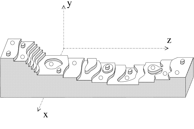
FIG. 1.: Schematic view of a crystal surface suffering various instabilities. Step-bunching, step-meandering, and island (or advacancy) formation are depicted.

Kinetic roughening has long been as a mystery. With regard to MBE growth on a high symmetry surface, a prominent example is the Kardar-Parisi-Zhang[4] equation introduced in an attempt to describe surface noise-induced-roughening, its one dimensional version is:

$$\partial_{t}y=a\Omega F+\partial_{xx}y+\left(\partial_{x}y\right)^{2}+\eta,$$ (1)

where $y$ is the surface height, and $x$ the coordinate along the surface(1). Derivatives are subscripted, that is $\partial_{t}y=\partial y/\partial t$ and so on. $F$ is the incoming flux, $a$ is the atomic height and $\Omega$ is the atomic area. We have set the coefficients to unity, since only the form of the equation matters in this discussion. This equation has given rise to a variety of investigations both analytically and numerically (this part has included analytical treatment of the partial differential equation together with numerical Monte-Carlo simulations which mimics KPZ dynamics). Equation (1) is phenomenological in the sense that it is derived on the basis of symmetries.

The KPZ nonlinearity is a natural candidate in the long wavelength limit, if desorption is present, or if allowance is made for defects (such as vacancies–often named overhangs– in the growing solid). No derivation of that equation has been given so far, however. The reason is, in our opinion, the lack of a continuum description of island nucleation. In the absence of both defects and desorption (which are two usual requirements for production of solids of interest!), the nonlinear KPZ term is not permissible[2]. In that case the equation must have a form of a conservation law, that is:

$$\partial_{t}y=a\Omega F-{\bf\nabla}.{\bf J},$$ (2)

oo that upon averaging, the mean velocity is simply be given by $a\Omega F$, as it should be; because the KPZ nonlinearity can not be written as a flux (i.e. as a divergence of a current) it gives an additional contribution to the grwoth velocity by a quantity $<(\partial_{x}y)^{2}>\neq 0$ (the symbol $<..>$ stands for to the average), which obviously makes no sense. There has thus been a variety of attempts with the aim of deriving the appropriate surface evolution equation in that limit. Here again no derivation from first principles is available.

As said above, in addition to surface roughness caused by shot noise, nominal high symmetry as well well as vicinal surfaces, may become inherently unstable[2] when brought away from equilibrium. Nominal surfaces may develop mounds due to the ES effect. However, derivation of the appropriate surface evolution equation in that case is still a matter of debate, though a significant progress has been achieved.

In contrast to nominal surfaces, vicinal surfaces in the step flow regime have allowed to derive evolution equations from first principles. In a series of papers, we have shown[5, 6, 1] that vicinal surfaces offer a relatively tractable situation, though often nontrivial, where evolution equations can be extracted from basic transport and kinetic laws. The strategy is to first focus on derivation of step evolution equations. Once this task is achieved, it becomes then possible to derive the surface evolution equation. In its general form, the evolution equation is nonlocal and highly nonlinear. A rather simple information is extracted, however, if we focus on the long-wavelength limit: that is we assume that the wavelength of the step meander, and thus surface modulation, is small in comparison to the natural physical length (diffusion length if desorption is important, otherwise the interstep distance, which is the most frequent situation). More precisely the full growth equations, which are highly nonlinear and nonlocal, can be reduced to nonlinear partial differential equations, which are more tractable and often allow a signficant analytical progress as wil be shown here.

As shown by Bales and Zangwill[7], a straight step during MBE growth may become morphologically unstable in the presence of an attachment asymmetry (the Ehrlich-Schwoebel (ES) effect) at the step. Close to the instability threshold, starting from the Burton-Cabrera-Frank (BCF)[8] model, we have shown[5] that the step profile in the presence of desorption obeys the Kuramoto-Sivahinsky equation (written in a canonical form):

$$\partial_{t}\zeta=-\partial_{xx}\zeta-\partial_{xxxx}\zeta+\left(\partial_{x}\zeta\right)^{2},$$ (3)

where $x$ is the coordinate along the step (Fig.1), and $\zeta$ designates the step position. In a similar fashion we have shown later that steps on a vicinal surface obey a set of coupled anisotropic Kuramoto-Sivahinsky equations[6]. The ultimate stage of surface dynamics is found to be spatiotemporal chaos. Two remarks are in order: (i) the KPZ nonlinearity is of the KS type –due to desorption– (ii) the first term in the KS equation has a negative sign, signalling an instability; there is a necessity for taking higher order derivatives into account in order to prevent arbitrary short wavelength modes to develop.

A question of major importance arose recently[1]: if desorption is negligible, what kind of nonlinearity should one expect? because of the conserved character of dynamics, only terms which can be written as derivatives of a current are allowed. We could naively have thought that a natural candidate would be the conserved KS equation, namely $\partial_{t}\zeta=-\partial_{xx}\zeta-\partial_{xxxx}\zeta+\partial_{xx}[\left(\partial_{x}\zeta\right)^{2}]$. A close inspection of the BCF equations, as shown here in details, reveals that this is not the case, though symmetry and conservation would dictate that form as the first plausible candidate. We have recently shown[1] that, for an in-phase train of steps, each step obeys the following nontrivial evolution equation:

$$\partial_{t}\zeta=-\partial_{x}\left[{1\over 1+(\partial_{x}\zeta)^{2}}\left(\partial_{x}\zeta+\partial_{x}\left({\partial_{xx}\zeta\over(1+(\partial_{x}\zeta)^{2})^{3/2}}\right)\right)\right].$$ (4)

This highly nonlinear equation could not be inferred from scaling and symmetry arguments. It is related to a singular behavior of the amplitude of the meander that behaves as $1/F^{1/2}$ when $F$ is small. Instead of chaos, a regular pattern is revealed, the modulation wavelength is fixed at the very initial stages while the amplitude of the step deformation follows a scaling law $w\sim t^{1/2}$.

The objective of this paper is many fold. We first give an extensive derivation of the above evolution equation starting from the BCF model. We shall also present a general argument on why that singular behavior is present in the absence of desorption. A second line of the investigation concerns higher order contributions. It is clear that the above equation enjoys the up-down symmetry, $\zeta\rightarrow-\zeta$. We show here that the effect of higher order contributions is to destroy this up-down symmetry. An important fact to be presented here is that the step profile exhibits a plateau-like morphology. This contradicts the preliminary simulation given in Ref. [1]. That simulation had suffered from numerical inaccuracy causing spurious spikes to develop. Finally we show that though the full equation is highly nonlinear it has been possible to provide a quantitative analytical treatment for the step morphology, and evaluate the plateau width along with the meander amplitude. The results are found to be in good agreement with numerical results.

This paper is organized as follow. We write down the basic equations in section II. In section III a linear stability analysis is performed, which allows to evaluate the most unstable wavelength and the typical time for the appearance of the instability. In section IV we shall provide a general argument on the extraction of the scaling of the step position with the incoming flux. Section V presents the detailed derivation of the principal evolution equation (4) in the one-sided limit. We shall then present the situation where there is a finite ES barrier. Section VI deals with the higher order terms and their impact on the up-down symmetry. In section VII we generalize the derivation of the step evolution equations to the two-sided case. Discussion and outlook are presented in section VIII.

II Basic equations

We present the model based on that of BCF, supplemneted with asymmetric attachment kinetics as introduced by Schwoebel [9], and line diffusion following Ref. [10]. A vicinal surface, whose mean interstep distance is $\ell$, is considered. On the terraces, the adatom concentration $c_{m}$ between steps $m$ and $m+1$ evolves according to:

$$\partial_{t}c_{m}=D\nabla^{2}c_{m}+F,$$ (5)

where $D$ is the adatom diffusion constant, $F$ is an incoming flux of adatoms from a beam, and $\partial_{t}$ denotes the time derivative. Once an atom is attached to the surface, it cannot detach from it (no desorption). We consider the widely used quasistatic limit where the concentration reaches a steady state regime on time scales much faster than that of step motion. We then have to solve Eq.(5) with the l.h.s. equal to zero. For implications due to non-quasisteady effects see Ref.[11].

The excursion of the $m^{th}$ step about its straight configuration is denoted $\zeta_{m}(x,t)$, so that its position is $m\ell+\zeta_{m}(x,t)+Vt$, where $V$ is the mean step velocity. We consider the case where no step overhang is present, so that the function $\zeta(x)$ is univocal. On both sides ($+$ and $-$ designate the lower terrace and the upper one respectively) of step $m$, the normal diffusion flux is linearly related to departure from equilibrium with kinetic coefficients $\nu_{\pm}$:

$$D\partial_{n}c_{m}|_{+} = \;\;\;\nu_{+}(c_{m}-c_{eq})|_{+}$$ (6)

$$D\partial_{n}c_{m-1}|_{-} = -\nu_{-}(c_{m-1}-c_{eq})|_{-},$$ (7)

where $c_{eq}$ is the local equilibrium concentration, and $\partial_{n}$ denotes the derivative in the direction which is normal to the step. More precisely $\partial_{n}\equiv{\bf n}.{\bf\nabla}$ where ${\bf n}=(-\zeta_{x},1)/\sqrt{1+\zeta_{x}^{2}}$ is the unit vector normal to the step, and ${\bf\nabla}$ is the two dimensional gradient operator: ${\bf\nabla}=(\partial_{x},\partial_{z})$ where $x$ is the coordinate along an originally straight step, and $z$ the one orthogonal to it. The attachment lengths on both sides of the steps will be used later: $d_{+}=D/\nu_{+}$ and $d_{-}=D/\nu_{-}$. If $c_{eq}^{0}$ is the adatom concentration close to a straight step, the concentration for a curved step is given by[5]:

$$c_{eq} = c_{eq}^{0}(1+\Gamma\kappa_{m}),$$ (8)

where $\Gamma=\Omega\tilde{\gamma}/k_{B}T$ (the definition of $\Gamma$ is slightly different from that of Ref. [12]) with $\tilde{\gamma}$ the step stiffness, and $\kappa_{m}$, the step curvature is given by:

$$\kappa_{m}=-{\partial_{xx}\zeta_{m}\over[1+(\partial_{x}\zeta_{m})^{2}]^{3/2}}.$$ (9)

Here for simplicity we disregard step-step elastic interaction. We shall come back to this point in the discussion.

At the steps, mass conservation, in the limit where the adatom concentration is much smaller than that of the solid $1/\Omega$, imposes:

$$V_{n}=\Omega\left(D\partial_{n}c_{m}|_{+}-D\partial_{n}c_{m-1}|_{-}\right)+a\partial_{s}[D_{L}\partial_{s}(\Gamma\kappa_{m})],$$ (10)

where $a$ is an atomic distance. Using Einstein’s relation, the macroscopic diffusion constant along steps is defined as $D_{L}=D_{st}ac_{st}$, where $D_{st}$ and $c_{st}$ are the diffusion constant and the concentration of mobile atoms along the step, respectively. This expression is in agreement with that of Mullins [13]. One may object that $c_{st}$ is in fact not well defined along a step. We shall therefore use a more general expression derived from the Kubo formula [14, 15, 16]: $D_{L}=a^{2}/\tau_{L}$ where $\tau_{L}$ is the characteristic time for detachment of an atom from a kink. Non-equilibrium effects related to line diffusion are not considered in this expression.

Two sources of nonlinearities can be identified. The first one is apparent in the boundary conditions (8, 10) because both the normal to the step and the curvature (see Eq.(9)) are nonlinear functions of the step profile. The second one originates the free boundary character (Stephan problem) is a hidden source of nonlinearity: the concentration field on a terrace –which is a nonlinear function of the position– depends on the step profile, leading thus to a nonlinear concentration field as a function of the step position.

In addition to elastic interactions (not included here), steps are coupled via adatom diffusion. Dynamics are nonlocal in space and time. With the help of an integral formulation of the model equations, we have made explicit this nonlocality in a previous work [3]. The use of the quasistatic approximation suppresses delay effects, whereas spatial nonlocality persists.

III Linear stability analysis

The linear stability analysis is the first step in any stability problem. Moreover it will allow us to prepare some preliminaries for the nonlinear analysis. Let us define the Fourier transform of the meander as:

$$\zeta_{\omega k\phi}=\sum_{m=-\infty}^{\infty}\int_{-\infty}^{+\infty}\int_{-\infty}^{+\infty}\,\,\zeta_{m}(x,t)\;e^{-i\omega t-ikx-i\phi m}\;dx\;dt,$$ (11)

where $i\omega$ is the pulsation of the perturbation of wavevector $k$ and phase shift between two neighboring steps, $\phi$. The phase varies between $0$ and $2\pi$. Let us quote two special cases. The in-phase mode $\phi=0$, corresponds to the case where all step meanders are identical, i.e. $\zeta_{m}(x,t)=\zeta_{m^{\prime}}(x,t)$ for any $m$, $m^{\prime}$. The out of phase mode $\phi=\pi$ corresponds to the situation $\zeta_{m}(x,t)=-\zeta_{m+1}(x,t)$.

The derivation of the full dispersion relation can be performed in this case along the same lines as in Ref.[17]. We shall not repeat here the calculation, but give directly the result. The quantity $i\omega$ is complex, and let us discuss separately the real and imaginary parts. The real part of $i\omega$ takes the form

$$\Re e(i\omega) = \Omega F\frac{q}{\cal D}\left(\frac{d_{-}-d_{+}}{\ell+d_{-}+d_{+}}\right)\left[(d_{-}+d_{+})\left(q\ell\;\sinh(q\ell)-\cosh(q\ell)+\cos(\phi)\right)+\frac{\ell}{2}q\ell\;\sinh(q\ell)\right]$$ (13)

$$-\Gamma q^{2}\left[D_{S}\frac{q}{{\cal D}}\left(2\left(\cosh(q\ell)-\cos(\phi)\right)+q(d_{+}+d_{-})\;\sinh(q\ell)\right)+aD_{L}q^{2}\right],$$

with $q=|k|$, and

$${\cal D} = (d_{+}+d_{-})q\cosh(q\ell)+(d_{+}d_{-}q^{2}+1)\sinh(q\ell).$$ (14)

Both macroscopic diffusion constants (adatom tracer diffusion constant $D$ times coverage of mobile atoms) on the terraces $D_{S}=D\Omega c_{eq}^{0}$ and $D_{L}$ along the steps enter this relation. The ”bare” (tracer) diffusion constant of adatoms on terraces does not appear alone.

A positive $\Re e(i\omega)$ is a signature of an instability. The straight step is unstable during growth provided that a normal ES effect is present ($d_{-}>d_{+}$). Moreover, the most unstable mode is the in-phase mode $\phi=0$. This remark will be exploited later.

The imaginary part of $i\omega$ describes propagative effects:

$$\Im m(i\omega)=\Omega F\sin(\phi)\frac{q}{\cal D}(\ell+d_{+}+d_{-}).$$ (15)

The origin of this term is quite transparent. In the limit of a straight step ($q=0$), we have $\Im m(i\omega)=\Omega F\sin(\phi)$, so that the perturbed solution takes the form (ignoring the real part of $i\omega$), $\zeta_{m}\sim e^{in\phi+it\Omega F\sin(\phi)}=e^{i\phi[n+t(V_{0}/\ell)\sin(\phi)/\phi]}$. Here we have introduced the step velocity of the uniform train, $V_{0}=\Omega F\ell$. This means that in order to travel a distance $n\ell$, it takes for a perturbation a time given by $(n\ell/V_{0})(\phi/\sin(\phi))$. Since $\phi/\sin(\phi)>1$, that time is always longer than that needed for a uniform train ($\phi=0$) to travel the same distance. In other words, all perturbations (except the in phase one) travel forward slower that the train velocity $V_{0}$. This means that perturbations are advected backwards in the reference frame with velocity $V_{0}$.

IV Scaling analysis

Once the instability threshold is reached, any perturbation will amplify exponentially in the course of time, so that nonlinear effects can no longer be disregarded. As discussed in section II, the set of growth equations is highly nonlinear and nonlocal, so that only a ”brute force” numerical analysis would give a general answer. Our idea is to inspect the original equations and try to reduce legitimately the complexity. The key ingredient in our analysis is the identification of a small parameter.

A Scaling of space and time variables

When inspecting the dispersion relation (13) for an in phase train, one realizes that the band of unstable wavenumbers extends from $q=0$ (actually this result is traced back to translational invariance; it corresponds to a global motion of the train) to a critical finite value $q_{c}$ (to be defined below). We shall assume that $q\ell$ remains small in comparison to one, and we come back in the discussion below to the validity of this assumption. In that case Eq.(13) takes a simpler form

$$Re[i\omega(q\ll 1,\phi=0)]={\Omega F\ell^{2}\over 2}{d_{-}-d_{+}\over\ell+d_{+}+d_{-}}q^{2}-(D_{S}\ell+D_{L}a)\Gamma q^{4}.$$ (16)

We have set here $\Phi=0$, which is the exploitation of the fact that the in-phase mode is the most dangerous one. We consider later the situation where small deviations from the in-phase mode are taken into account. It is seen that the range of wavenumbers with positive $i\omega$ is given by

$$q_{c}=\left({\Omega F\ell^{2}f_{s}\over\Gamma(D_{S}\ell+D_{L}a)}\right)^{1/2},$$ (17)

where $f_{s}=(d_{-}-d_{+})/(\ell+d_{+}+d_{-})$ is a parameter describing the Ehrlich-Schwoebel effect. The demand that the small wavenumber expansion make a sense is satisfied by requiring $\epsilon\equiv(q_{c}\ell)^{2}\ll 1$, and this is precisely the definition of our small parameter

$$\epsilon={\Omega Ff_{s}\ell^{4}\over\Gamma(D_{S}\ell+D_{L}a)}.$$ (18)

This guarantees the long wavelength regime. It is important to see from the very beginning whether this limit is realistic, or is it rather academic. Experimental data are available on vicinal surfaces of $Cu(1,1,17)$ which have recently revealed a meandering instability during step-flow growth[18]. Their data entering the expression of $\epsilon$ which are best known are $\Omega F=3\;10^{-3}s^{-1}$, $\ell=21.7\AA$. The step stiffness can be written as $\tilde{\gamma}\approx(k_{B}T/2a)\exp(E_{k}/k_{B}T)$, $E_{k}$ being the kink energy. From a simple ”bond counting” argument, one can evaluate the adatom equilibrium concentration on a vicinal surface: $\Omega c_{eq}^{0}\sim\exp(-E_{a}/k_{B}T)$ with $E_{a}=3E_{k}$. Using the result of Ref. [15, 16] from step fluctuations at equilibrium, we have $E_{k}=0.13eV$. The diffusion constant on terraces takes the form $D=a^{2}\nu_{0}\exp(-E_{D}/k_{B}T)$, $\nu_{0}\sim 10^{13}s^{-1}$ is an intrinsic frequency, and $E_{D}\approx 0.45eV$ [19]. With a lattice constant of $2.55{\rm\AA}$, we find: $D_{S}\ell=1.4\times 10^{15}\exp(-0.84{\em eV}/k_{B}T)$.

Using the Kubo formula [14], one can evaluate the line diffusion constant: $D_{L}=a^{2}/\tau_{L}$. From experimental data [15, 16]: $D_{L}a=aD_{L0}\exp(-E_{L}/k_{B}T)$, with $aD_{L0}=6.5\times 10^{18}{\rm\AA}^{2}s^{-1}$ and $E_{L}=0.89eV$. With these values, we find that $D_{S}\ell/(D_{L}a)\sim 10^{-2}$ in the experimental temperature range. This indicates that the stabilization of steps essentially occurs via line diffusion in this situation. In the one-sided limit ($d_{+}=0$ and $d_{-}\rightarrow\infty$), and around $300K$ we find $\epsilon\sim 10^{-3}$, and $\lambda_{c}=2\pi/q_{c}\sim 10^{3}$ atomic distances. This result implies that a priori the longwavelenggth limit is appropriate.

The active modes in the instability are those for which $q\ell\sim q_{c}\ell\sim\epsilon^{1/2}$, and therefore, lengthscales of interest are those for which $x\sim\ell\epsilon^{-1/2}$. The characteristic time of the instability development is given by the growth rate of the most unstable mode:

$$t_{m}\sim{2\pi\ell^{4}\over\Gamma(D_{S}\ell+D_{L}a)}\;\epsilon^{-2}.$$ (19)

This is obtained as $t_{m}\equiv 2\pi/\Re e[i\omega(q=q_{m},\phi=0)]$, $q_{m}$ being the wavevector of the most unstable mode, related to $q_{c}$ by $q_{m}=q_{c}/\sqrt{2}$. This relation provides the scaling of the time variable $t\sim\epsilon^{-2}$. Using the above data, we find that the instability typically develops after a growth of a thickness of the order of $100$ monolayers.

Before proceeding further, it is instructive to analyze briefly the asynchronized train. As pointed out in an earlier work [1], the ES effect not only induces a morphological instability of steps, but also leads to a “diffusive repulsion” between steps on a vicinal surface. This dynamical repulsion will force steps to evolve in-phase. The time needed for steps to organize in-phase in the unstable train is $t_{\phi}$, defined as the synchronization time of the most unstable mode with wavevector $q=q_{m}=q_{c}/\sqrt{2}$ (i.e. the on e having the maximum growth rate):

$${1\over t_{\phi}}\sim\partial_{\phi\phi}\Re e\left[\omega(q,\phi)|_{q=q_{m},\phi=0}\right].$$ (20)

This time corresponds to the decay of a perturbation having phase shifts of order one. From linear dispersion relation (Eq.13):

$${t_{\phi}\over t_{m}}\sim\epsilon\left({(\ell+d_{+}+d_{-})(D_{S}\ell+D_{L}a)\over D_{S}\ell(d_{-}+d_{+}+\ell/2)+D_{L}a(d_{-}+d_{+})}\right),$$ (21)

where $t_{m}$ is the typical time for the instability to develop (Eq.(19)). In the one-sided limit, $t_{\phi}/t_{m}\sim\epsilon$. Thus, we expect the synchronization time to be shorter than the instability time, i.e. $t_{\phi}/t_{m}\ll 1$ since $\epsilon\ll 1$. This means that steps will be synchronized in the early stage of the instability. This justifies the fact to focus on small phases, or possibly a vanishing phase, as we shall assume later.

For small but finite $\phi$ we have

$$\Re e[i\omega(q\ll 1,\phi\ll 1)]= - {\Omega F\over 2}{d_{-}-d_{+}\over\ell+d_{+}+d_{-}}\left((q\ell)^{2}-{d_{+}+d_{-}\over\ell+d_{+}+d_{-}}\phi^{2}\right)$$ (22)

$$- \left((D_{S}\ell+D_{L}a)q^{2}+{D_{S}\over\ell+d_{+}+d_{-}}\phi^{2}\right)\Gamma q^{2}.$$ (23)

It is seen from the first term that for the phase shift to be relevant we must have $\phi\sim q\ell\sim\epsilon^{1/2}$. This implies that the conjugate variable $m$ (the step position along the vicinality) has the following scaling $m\sim\epsilon^{-1/2}$ (meaning that one needs to travel a distance of that order to detect phase modulations). In summary we have the following scaling in Fourier space

$$q\sim\epsilon^{1/2},\;\;\;\;\omega\sim\epsilon^{2},\;\;\;\;\phi\sim\epsilon^{1/2},$$ (24)

and their corresponding conjugate variables in real space

$$x\sim\epsilon^{-1/2},\;\;\;\;t\sim\epsilon^{-2},\;\;\;\;m\sim\epsilon^{-1/2}.$$ (25)

Beside the instability character, the problem involves progative effects which are related to the imaginary part of $i\omega$. Inspection of the imaginary part of the dispersion relation (15) in the long wavelength and small $\phi$ limit, shows that $\Im m(i\omega)\sim\epsilon^{3/2}$. This defines a fast timescale $\tau\sim\epsilon^{-3/2}$ related to propagative effects –we mean faster than the time scale associated with the instability $\sim\epsilon^{-2}$. Since we shall mainly be interested by a synchronized train (in which case the imaginary part vanishes), we shall leave out this additional complication for the moment, and postpone this question to a forthcoming work.

B Scaling of the meander

In order to determine the nonlinear evolution equation, following our previous work[5] in the presence of desorption, we could expand all physical quantities (concentration, step position) in power series of the small parameter, the leading contribution would be of order $\epsilon^{0}$, followed (in principle, and in a regular expansion) by $\epsilon^{1/2}$, since this is the smallest power encountered above. This strategy worked out when desorption is present, but not in the present context. The reason is that the first contribution in the step profile turned out to be $\zeta\sim\epsilon^{-1/2}$. This was viewed as an ansatz in our previous work [1]. In this paper we provide an explanation of that fact on the basis of general considerations. Without having resort to an explicit derivation we shall show why this scaling is inherently linked with the non-desorption case.

For that purpose it is useful to identify two ’classes’ of adatoms (of course just in terms of a picture): Thermal adatoms of concentration $c_{T}$ detach from a step, diffuse on terraces and re-attach to a step. Mass transport associated to their motion induces relaxation towards equilibrium. Freshly landed adatoms of concentration $c_{F}$ have not yet been incorporated into a step. Their attachment result in the non-equilibrium driving of the steps. We can thus split the full set of equations (5-10) into two pieces by writing the model equations in the following equivalent form:

$$D\nabla^{2}c_{T} = 0,$$ (26)

$$D\nabla^{2}c_{F} = -F.$$ (27)

These fields obey the following boundary conditions at the steps:

$$D\partial_{n}c_{T} = \pm\nu_{\pm}(c_{T}-c_{eq}),$$ (28)

$$D\partial_{n}c_{F} = \pm\nu_{\pm}c_{F},$$ (29)

where the index $+$ and $-$ refer to both sides of the steps. They are coupled only through mass conservation at the steps

$$V_{n} = v_{F}+v_{T},$$ (30)

where the driving contribution $v_{F}$ is proportional to the incoming flux $F$:

$$v_{F}=D[\partial_{n}c_{F_{+}}-\partial_{n}c_{F_{-}}].$$ (31)

Indeed from the equations obeyed by $c_{F}$ (Eqs.(27), (29)) by making the transformation $c_{F}\rightarrow c_{F}/F$ one sees that $F$ scales out from the equations, implying thus that $c_{F}$ must directly be proportional to $F$.

We can extract from $c_{F}$ the contribution of the uniform train, which leads to a velocity given by $\Omega F\ell$, plus another contribution due to step modulations which must be compatible with conservation. $v_{F}$ is thus the sum of the mean step velocity and the divergence of a flux $j$ that describes how mass is unequally distributed between different steps, and different parts of each step:

$$v_{F}=\Omega F(\ell-\nabla j),$$ (32)

with $j$, according to what is stated above, independent of $F$.

The relaxational contribution $v_{T}$ is a thermal part and is obviously independent of $F$:

$$v_{T} = [D\partial_{n}c_{T}]^{+}_{-}+a\partial_{s}[D_{L}\partial_{s}\Gamma\kappa].$$ (33)

Gradients of chemical potential $\mu$ are the driving force of the relaxational contribution. Without loss of generality, and as long as we deal with smooth and large scale perturbations, the thermal part of the normal velocity can be written with help of the Cahn-Hilliard [20] equation:

$$v_{T}=\nabla[{\bf M}\nabla\mu],$$ (34)

where ${\bf M}$ is the macroscopic mobility of the surface, and $\mu=\Omega\tilde{\gamma}\kappa$ is the chemical potential. The step index $m$ is omitted in this section to simplify notations. Thus we shall from now on use the scalar mobility $M$ along $x$. The chemical potential is expressed as $\mu=\Omega\delta{\cal F}/\delta\zeta$, where ${\cal F}$ is the step free energy. Thus, if $f(\partial_{x}\zeta)$ is the free energy density, we have:

$$\mu=-{d\over dx}[f^{\prime}(\partial_{x}\zeta)].$$ (35)

The evolution equation of the step meander (i.e. when the step mean velocity is subtracted) now reads:

$$\partial_{t}\zeta=-\partial_{x}\left[\Omega Fj+M\partial_{xx}f^{\prime}\right].$$ (36)

Recall that $F$ is proportional to $\epsilon$ (Eq.(18)), so that we can set $F=\epsilon\bar{F}$, where $\bar{F}$ is of order one. On the other hand $x=X\epsilon^{-1/2}$ (Eq.(25)), so that $\partial_{xx}=\epsilon\partial_{XX}$. $j$, $M$ or $f^{\prime}$ only depend on derivatives of $\zeta$, due to translational invariance. We write their argument symbolically as $\{\partial_{x}\}=\{\epsilon^{1/2}\partial_{X}\}$ (which is taken to mean any derivative and any power). Equation (36) can be rewritten as:

$$\partial_{t}\zeta=-\epsilon^{3/2}\partial_{X}\left[\Omega\bar{F}j\{\epsilon^{1/2}\partial_{X}\}+M\{\epsilon^{1/2}\partial_{X}\}\partial_{XX}f^{\prime}\{\epsilon^{1/2}\partial_{X}\}\right].$$ (37)

The central point lies in the fact that the small parameter $\epsilon$ appears as a common factor, in the first term it stems from $F$ while in the second one it originates from the second spatial derivative.

In a regular expansion, close to the instability point we expect that the amplitude of modulation is vanishingly small when $\epsilon\ll 1$. In reality, and this is the heart of the proof, due to the structure of the above equation, it will follow that no nonlinear term can enter the evolution equation, even if the amplitude were allowed to be of order one. There is even a stronger statement. Indeed even if $\zeta=\epsilon^{\vartheta}H$ ($H$ is of order one), with $\vartheta>-1/2$, we show below that any nonlinear term has a vanishing contribution. For that purpose we expand any function noted $h$ (which represents $j$….) in a Taylor series

$$h=h_{0}+h_{1}\epsilon^{1/2+\vartheta}(\partial_{X}H)+h_{2}\epsilon^{1+2\vartheta}(\partial_{X}H)^{2}+{\rm h.o.t.},$$ (38)

where we have kept the smallest linear and nonlinear terms. For example a term like $\epsilon^{\vartheta+1}\partial_{XX}H\ll\epsilon^{\vartheta+1/2}\partial_{X}H$. Although our conclusion can be made at this stage, let us be more explicit. Setting $T=\epsilon^{2}t$, Eq.(36) now reads:

$$\epsilon^{\vartheta+2}\partial_{T}H=-\epsilon^{\vartheta+2}\partial_{X}\Bigl{[}j_{1}\partial_{X}H+\epsilon^{\vartheta+1/2}j_{2}(\partial_{X}H)^{2}$$ (39)

$$+\left(M_{0}+\epsilon^{\vartheta+1/2}M_{1}\partial_{X}H\right)\partial_{XX}\left(f_{1}^{\prime}\partial_{X}H+\epsilon^{\vartheta+1/2}f_{2}^{\prime}(\partial_{X}H)^{2}\right)\Bigr{]}+{\rm h.o.t.},$$ (40)

Since $\vartheta>-1/2$, we have $\epsilon^{\vartheta+1/2}\rightarrow 0$ as $\epsilon\rightarrow 0$. Therefore, nonlinear terms are irrelevant in Eq.(40), and the full equation reduces to a linear evolution equation:

$$\partial_{T}H=-\left(j_{1}\partial_{XX}H+M_{0}f_{1}^{\prime}\partial_{XXXX}H\right).$$ (41)

For nonlinearities to be relevant in Eq.(40), we need $\epsilon^{\vartheta+1/2}\sim O(1)$, which is obtained when $\vartheta=-1/2$. But then, the expansion performed in Eq.(38) is a priori not legitimate. Indeed, higher order terms become relevant: $(\partial_{x}\zeta)^{n}\sim\epsilon^{n(\vartheta+1/2)}\sim O(1)$ when $\vartheta=-1/2$ for any integer $n$. We therefore expect a highly nonlinear evolution equation, as will be shown explicitly in the next section.

How concentration scales with $\epsilon$ can also be found using the decomposition of the concentration. From equations (27) and (29), we have $c_{F}\sim F\sim\epsilon$. From Eq.(26), (28), and (8), we find that

$$c_{T}-c_{eq}^{0}\sim c_{eq}-c_{eq}^{0}\sim c_{eq}^{0}\Gamma\kappa\sim\epsilon^{1/2}.$$ (42)

Thus, $u=\Omega{c_{F}+c_{T}-c_{eq}^{0}}\sim\epsilon^{1/2}$, and the concentration will be written in the following form:

$$u(x,t) = \epsilon^{1/2}U(x,t),$$ (43)

with $U(x,t)\sim O(1)$. Similarly, the meander will be written as:

$$\zeta(x,t) = \epsilon^{-1/2}H(x,t),$$ (44)

where $H(x,t)\sim O(1)$.

It is important to show why in the presence of desorption the expansion is regular, leading to the KS equation ([5]). With desorption the evolution equation can no longer be written in the form of a conservation law (2). Nevertheless, the above mentioned decomposition still holds in a slightly different form: instead of being proportional to $F$, the driving part is proportional to $F-F_{eq}$, where $F_{eq}$ is the incoming flux at equilibrium that counterbalances ambiant desorption ($F_{eq}=c_{eq}^{0}/\tau$, $\tau$ being the characteristic residence time before desorption on a terrace). Hence, instead of Eq.(36), we have:

$$\partial_{t}\zeta=(F_{eq}-F)g+N\;\partial_{xx}f^{\prime},$$ (45)

where $g$ and $N$ are functions of the derivatives of $\zeta$. The second term of the r.h.s. is now the one expected for non-conserved relaxation to equilibrium: it is directly proportional to the chemical potential variations (See model A in Ref. [21], or [13]). Linearizing this equation, we have to take $g\approx\tilde{g}\partial_{xx}\zeta$ since the first linear term proportional to $\partial_{x}\zeta$ is a propagative term, not contributing to stabilization or destabilization (moreover, this term, not invariant under the $x\rightarrow-x$ symmetry, is not allowed). We then find:

$$\partial_{t}\zeta=[(F_{eq}-F)\tilde{g}+N_{0}f^{\prime}_{1}]\;\partial_{xx}\zeta.$$ (46)

The prefactor of $\partial_{xx}\zeta$ is the effective stiffness of the step. An instability is signaled by a negative sign of that prefactor. This happens when $F>F_{c}=F_{eq}+N_{0}f^{\prime}_{1}/\tilde{g}$. The small parameter (that is the distance from the instability threshold) is now $\epsilon^{\prime}\sim F-F_{c}$. Moreover it was found in Ref. [5, 12] that $x\sim\epsilon^{\prime-1/2}$ and $t\sim\epsilon^{\prime-2}$. Defining as in the conserved case $X=\epsilon^{\prime 1/2}x$ and $T=\epsilon^{\prime 2}t$, and $\zeta=\epsilon^{\prime\vartheta^{\prime}}H$, with $X,T,H\sim O(1)$, Eq.(45) is now expanded for $F\approx F_{c}$ as:

$$\epsilon^{\prime\vartheta^{\prime}+2}\;\partial_{T}H=-\epsilon^{\prime\vartheta^{\prime}+2}\;\tilde{g}\;\partial_{XX}H+\epsilon^{\prime 2\vartheta^{\prime}+1}\;(F-F_{eq})\;(\partial_{X}H)^{2}\;g_{2}$$ (47)

$$+\epsilon^{\prime 2\vartheta^{\prime}+2}\;\left[N_{0}\,f_{2}^{\prime}\,\partial_{XX}\,(\partial_{X}H)^{2}+N_{1}\,f_{1}^{\prime}\,\partial_{X}H\,\partial_{XXX}H\right]+{\rm h.o.t.}.$$ (48)

As before, we use $\vartheta^{\prime}>-1/2$ so that expansion (38) makes a sense. It is seen from this equation that the leading nonlinear term is $(F-F_{eq})\,\epsilon^{\prime 2\vartheta^{\prime}+1}\,(\partial_{X}H)^{2}$. It counterbalances the linear term $\epsilon^{\prime\vartheta^{\prime}+2}\,\tilde{g}\,\partial_{XX}H$ provided that $\vartheta^{\prime}=1$. The nonlinear term here, is that of the Kardar-Parisi-Zhang [22] and Kuramoto-Sivashinsky [5, 3] equations (see Eq.(1) and (3)). It could not be present in the conserved case because it cannot be written as the divergence of a flux. Moreover, it is non-variational, and thus it must vanish at equilibrium, as can bee seen from its prefactor $F-F_{eq}$.

It must be emphasized that the decomposition into an equilibrium an a nonequilibrium part holds in the present problem, but is not a general property. This does not have to be the case out of equilibrium in general (an example is that of step flow or sublimation in the presence of electromigration, such a decomposition between relaxation and driving parts has not been made possible).

V One-sided synchronized steps

A Multiscale analysis

In addition to synchronization, we first assume for simplicity a one-sided limit (steps advance only thanks to atoms from the terrace which is ahead), formally defined as $d_{+}=0$, and $d_{-}\rightarrow+\infty$. In this limit Eq.(7) reduces to $c_{+}=c_{eq}$ (which is the Gibbs-Thomson condition) and $\partial c_{-}/\partial n=0$ (atoms do not descend the steps).

As we have shown in the last section the meander $\zeta\sim\epsilon^{-1/2}$, while the concentration field $u\sim\epsilon^{1/2}$, we find it convenient to set $\zeta=\epsilon^{-1/2}H$ and $u=\epsilon^{1/2}U$, with $H$ and $U$ being quantities of order one. Under the assumption that these quantities are analytic functions of $\epsilon^{1/2}$, we seek solutions of the form

$$U = U^{(0)}+\epsilon^{1/2}U^{(1/2)}+\epsilon U^{(1)}+\epsilon^{3/2}U^{(3/2)}+\cdots,$$ (49)

$$H = H^{(0)}+\epsilon^{1/2}H^{(1/2)}+\epsilon H^{(1)}+\epsilon^{3/2}H^{(3/2)}+\cdots.$$ (50)

In order to make explicit the $\epsilon$ dependence, and to deal with quantities of order 1, and according to (25), we set:

$$x=\epsilon^{-1/2}X,\;\;\;\;\;\;\;t=\epsilon^{-2}T$$ (51)

It is convenient to rescale space by $\ell$ and time by $D/\ell^{2}$. Performing the variable change: ${\cal Z}=z-\zeta_{m}(x,t)$, mass conservation (5) on terraces reads:

$$0={\rho^{2}}\;\;\partial_{{\cal Z}{\cal Z}}U+\;\epsilon^{1/2}\left(\eta-2\partial_{X}H\;\;\partial_{X{\cal Z}}U-\partial_{XX}H\;\;\partial_{{\cal Z}}U\right)+\;\epsilon\;\partial_{XX}U,$$ (52)

where $\rho=[1+(\partial_{X}H)^{2}]^{1/2}$, an $\eta=\epsilon\;D/\Omega F\ell^{2}$. At the steps, the Gibbs-Thomson relation at ${\cal Z}=0$, and a zero-flux condition at ${\cal Z}=1$, takes the form:

$$U|_{{\cal Z}=0} = -{\cal K},$$ (53)

$$\rho^{2}\partial_{\cal Z}U|_{{\cal Z}=1} = \epsilon^{1/2}\;\;\partial_{X}H\;\;\partial_{X}U\;\;|_{{\cal Z}=1}\;,$$ (54)

where ${\cal K}=\Omega c_{eq}^{0}\;\Gamma\;\partial_{XX}H/\rho^{3}$.

Mass conservation at the step (Eq.(10)) yields

$$V+\epsilon^{3/2}\partial_{T}H={\rho^{2}}\;\partial_{\cal Z}U|_{{\cal Z}=0}-\epsilon^{1/2}\;\partial_{X}H\;\;\partial_{X}U|_{{\cal Z}=0}-\epsilon^{3/2}\;\partial_{X}\left({\beta\over\rho}\partial_{X}{\cal K}\right),$$ (55)

where $\beta=D_{L}a/D_{S}\ell$. The strategy is now to solve equations (52-55) in successively higher orders in $\epsilon$.

order 0

To this order, Eq.(52) reads:

$$\partial_{{\cal Z}{\cal Z}}U^{(0)}=0,$$ (56)

which is solved by $U^{(0)}=A^{(0)}{\cal Z}+B^{(0)}$. Equations (53) and (54) provide two conditions from which we get $A^{(0)}=0$ and $B^{(0)}=-{\cal K}^{(0)}$. No contribution to step velocity is found to $0^{th}$ order. That is to say this order corresponds to the equilibrium case.

order 1/2

From (52) we find that $U^{(1/2)}$ obeys an inhomogeneous equation on terraces:

$$\rho^{(0)2}\partial_{{\cal Z}{\cal Z}}U^{(1/2)}=-\eta,$$ (57)

whose general solution takes the form:

$$U^{(1/2)}=\frac{-{\cal Z}^{2}}{2\rho^{(0)2}}\;\eta+A^{(1/2)}{\cal Z}+B^{(1/2)}.$$ (58)

From boundary conditions at the steps (53) and (54):

$$U^{(1/2)} = B^{(1/2)}=-{\cal K}^{(1/2)}$$ (59)

$$\rho^{(1/2)2}\;\partial_{\cal Z}U^{(1/2)}|_{{\cal Z}=1} = \partial_{X}H^{(0)}\;\partial_{X}B^{(1/2)}.$$ (60)

Integration constants are found to be:

$$A^{(1/2)} = (\eta-\partial_{X}H^{(0)}\;\partial_{X}{\cal K}^{(0)})\;/\;\rho^{(0)^{2}},$$ (61)

$$B^{(1/2)} = -{\cal K}^{(1/2)}.$$ (62)

Mass conservation at the step (55) determines the mean step velocity. Going back to physical variables, we find the expected result: $V=\Omega F\ell$.

order 1

To this order, $U^{(1)}$ obeys:

$$\partial_{{\cal Z}{\cal Z}}U^{(1)} = \frac{1}{\rho^{(0)^{2}}}\left[\partial_{XX}H^{(0)}\;\partial_{\cal Z}U^{(1/2)}+2\partial_{X}H^{(0)}\;\partial^{2}_{X{\cal Z}}U^{(1/2)}\right.$$ (64)

$$\left.-2\partial_{X}H^{(0)}\;\partial_{X}H^{(1/2)}\;\partial_{{\cal Z}{\cal Z}}U^{(1/2)}-\partial_{XX}U^{(0)}\right]$$

$$= a+b{\cal Z},$$ (65)

whose general solution takes the form:

$$U^{(1)}=\frac{b}{6}{\cal Z}^{3}+\frac{a}{2}{\cal Z}^{2}+A^{(1)}{\cal Z}+B^{(1)}.$$ (66)

Once again, integration factors $A^{(1)}$ and $B^{(1)}$ are found from boundary conditions (53) and (54):

$$U^{(1)}|_{{\cal Z}=0} = B^{(1)}=-{\cal K}^{(1)},$$ (67)

$$\partial_{\cal Z}U^{(1)}|_{{\cal Z}=1} = {b\over 2}+a+A^{(1)}$$ (68)

$$= \frac{1}{\rho^{(0)^{2}}}\left[\partial_{X}H^{(0)}\;\partial_{X}U^{(1/2)}\right.$$ (69)

$$+ \partial_{X}H^{(1/2)}\;\partial_{X}U^{(0)}$$ (70)

$$- \left.2\;\partial_{X}H^{(0)}\;\partial_{X}H^{(1/2)}\;\partial_{\cal Z}U^{(1/2)}\right]|_{{\cal Z}=1}.$$ (71)

Finally, mass conservation (55) leads to the sought after evolution equation for $H^{(0)}$:

$$\partial_{T}H^{(0)} = \partial_{\cal Z}U^{(1)}\rho^{(0)2}-\partial_{X}U^{(1/2)}\partial_{X}H^{(0)}-\partial_{X}\left({\beta\over\rho^{(0)}}\partial_{X}{\cal K}^{(0)}\right).$$ (72)

Upon substitution of the expressions of $U^{(1)}$ and $U^{(1/2)}$, one realizes that terms containing $H^{({1/2})}$ cancel exactly in this expression, leading to a closed form for the evolution equation for $H^{(0)}$:

$$\partial_{T}H^{(0)} =-\partial_{X}\left[\eta\frac{\partial_{X}H^{(0)}}{2\;\rho^{(0)^{2}}}+\left(1+\beta\rho^{(0)}\right)\frac{\partial_{X}{\cal K}^{(0)}}{\rho^{(0)^{2}}}\right].$$ (73)

Going back to physical variables, we obtain:

$$\partial_{t}\zeta=-\partial_{x}\left[\frac{\Omega F\ell^{2}}{2}\frac{\partial_{x}\zeta}{(1+(\partial_{x}\zeta)^{2})}-\left(D_{S}\ell+D_{L}a(1+(\partial_{x}\zeta)^{2})^{1/2}\right)\frac{\partial_{x}(\Gamma\kappa)}{(1+(\partial_{x}\zeta)^{2})}\right].$$ (74)

Besides the term proportional to $D_{L}$ (line diffusion constant), this is the equation derived in Ref.[1] on which we have given a brief account.

Introducing the step macroscopic mobility ${\cal M}$, and the chemical potential $\mu=k_{B}T\Gamma\kappa$, the evolution equation can be rewritten in a more compact and enlightening form:

$$\partial_{t}\zeta=-\partial_{x}\left[\frac{\Omega F\ell_{\perp}^{2}}{2}\partial_{x}\zeta-{\cal M}\partial_{s}\mu\right],$$ (75)

where $s$ is the arclength along the steps, and $\ell_{\bot}=\ell/[1+(\partial_{x}\zeta)^{2}]^{1/2}$ is the distance between two neighboring steps measured along their normal (see Fig.2 for geometrical definitions.). The effective step mobility reads:

$${\cal M}={D_{S}\ell_{\perp}+D_{L}a\over k_{B}T}.$$ (76)

The expected decomposition of step velocity (see section IV B) is clearly seen here. The first term on the r.h.s. of Eq.(75) is the driving part. To this term a simple geometrical meaning can be assigned (see Appendix A). The second term is the relaxation part with a mobility depending on the local step orientation. Note that the present mobility ${\cal M}$ and the one introduced in section IV B, noted $M$, differ by the scale factor $[1+(\partial_{x}\zeta)^{2}]^{1/2}$ which relates the arc-length $s$ to the Cartesian coordinate $x$.

B Numerical solution

In Ref [1], numerical solution of Eq.(74) (without line diffusion) was performed using a simple Euler scheme, and it was found that: (i) A cellular structure takes place, the wavelength of which (the most unstable one) is fixed at the initial stage of the instability and no coarsening is seen. (ii) The amplitude grows like $t^{1/2}$. (iii) The shape of the cells is similar to the inverse error function, that is to say it develops a spike-like morphology. (iv) The meander is symmetric with respect to the transformation $\zeta\rightarrow-\zeta$. It has been realized meanwhile that, though all these qualitative features were correct, the spikes are the result of a numerical deficiency in the original code. In order to cure this problem we have to resort to a special numerical treatment. Different successful attempts have been made but we shall here describe only the most robust numerical treatment.

We use a powerful geometrical representation of the meander [23, 24], in terms of the arclength $s$ and the angle $\theta$, oriented counterclockwise, between the normal and a given fixed direction (the z-axis direction) (see Fig.2). $\theta$ is related to $\zeta$ via: $\tan(\theta)=-\partial_{x}\zeta$ and the curvature simply reads: $\kappa=\partial_{s}\theta$.

FIG. 2.: Some definitions of the notations used in the text.

Simple differential geometry[24] provides us with the evolution equation for $\theta$, as a function of tangential and normal velocities, $v_{t}$ and $v_{n}$:

$$\frac{\partial\theta}{\partial t}=v_{t}\kappa-\frac{\partial v_{n}}{\partial s}.$$ (77)

Physics is invariant under a change of definition of the arclength $s$. This allows an arbitrary time-dependent re-parameterization of the curve. This ”gauge” can be seen as an additional tangential velocity,[23, 24] with no physical relevance. A particular choice that is convenient here is the one that keeps the relative arclength $s/L$ constant in the course of time, where $L$ is the total length of the curve. This will ensure that the discretization points remain equally spaced along the curve. The tangential velocity reads[23, 24]:

$$v_{t}=\frac{s}{L}\int_{0}^{L}\kappa v_{n}ds^{\prime}-\int_{0}^{s}\kappa v_{n}ds^{\prime}.$$ (78)

The evolution equation of the meander (74) allows one to write the step normal velocity:

$$v_{n}=-\partial_{s}\left[\cos(\theta)\;\sin(\theta)+\left(\frac{\beta+\cos(\theta)}{\beta+1}\right)\;\partial_{s}\kappa\right],$$ (79)

where time $t$ is rescaled by $4\ell^{4}/\epsilon^{2}\Gamma(l\;D_{S}+a\;D_{L})$ and spatial variables $x,\zeta,$ by $\sqrt{2}\ell/\sqrt{\epsilon}$, so that only one parameter survives: $\beta=D_{L}a/D_{S}\ell$.

Derivatives along the arclength $s$ are evaluated using a centered finite difference method. We use a backward differentiation scheme with variable step for time integration. This ”solver” enjoys rather good precision and L-stability (that is to say it is unconditionally stable and optimally attenuates high-frequency (i.e. noise) components of the solution) that makes it well fitted to our specific problem.

Our present simulations show qualitatively similar behavior as that found in Ref. [1] (see Fig.6). A major difference is revealed however: instead of spikes, the cellular structure exhibits a plateau in the extrema regions [25], as shown on Fig.3. (Here we define a plateau as a region of finite slope, as opposed to regions where the slope diverges with time. Hence, to some scale, plateaus are curved, and this curvature does not tend to zero). The width of a ”plateau” reaches a constant value after a transient regime.

FIG. 3.: Numerical solution of Eq.(64). Meander over one period. Cells are symmetric and develop plateaus. Their amplitude increases with time.

C Analytical study

We show here that the above numerical results can be accounted for using simple analytical arguments. We give here only the main results, whereas details are relegated into Appendix B. The central assumption is a decomposition in two types of regions, where two different ansatz are used. In the large slope regions, a multiplicative variable separation is used:

$$\zeta_{s}(x,t)=A(t)g(x),$$ (80)

while and additive variable separation is performed for the plateau regions:

$$\zeta_{p}(x,t)=B(t)+h(x).$$ (81)

An additional constraint coming from mass conservation allows to determine quantitatively the asymptotic behavior by matching these two solutions. The amplitude of the meander is found to behave as:

$$\zeta_{max}-\zeta_{min}=2a_{0}t^{1/2},$$ (82)

where $a_{0}$ is calculated in Appendix B. The rescaled meander $\zeta(x,t)/t^{1/2}$ converges to a well defined profile, and looks as if plateaus were formed in the extrema regions. The width of a plateau is defined as $\lambda_{0}/2$. We find:

$$\lambda_{0}=\lambda_{c}I(\tilde{\beta}),$$ (83)

where $\tilde{\beta}=D_{S}\ell/(D_{S}\ell+D_{L}a)$, $\lambda_{c}=2\pi/q_{c}$ is the largest stable wavelength from linear analysis, and $I$ is a function given in Appendix B. Since $I(\tilde{\beta})$ decreases monotonously from $I(0)=1$ to $I(1)\approx 0.54$, the plateau size increases as line diffusion is increased, and is always smaller than $\lambda_{c}/2$. Good quantitative agreement between the numerical solution of Eq.(74) and these analytical predictions is found (see Fig.4).

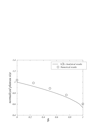
FIG. 4.: One sided case: The prediction for the normalized plateau size $I(\tilde{\beta})$ (solid line) is compared with numerical solution of Eq.(64) (symbols), which corresponds to the one-sided limit.

VI Front-Back symmetry breaking

The expansion performed in section V A can be pushed to next order following the same strategy. We shall here merely give the result and details can be found in Ref. [26]. Instead of a closed equation for $H^{(0)}$, here two coupled dynamical equations for $H^{(0)}$ and $H^{(1/2)}$ are obtained. Going back to the physical quantity $\zeta=\epsilon^{-1/2}(H^{(0)}+\epsilon^{1/2}H^{(1/2)})$, the coupled equations can be recast into a single equation for $\zeta$:

$$\partial_{t}\zeta = -\frac{\partial}{\partial x}\left[\frac{\Omega\;F\;\ell_{\perp}^{2}}{2}\partial_{x}\zeta\left(1-\frac{\kappa\;\ell}{3}\left(\frac{\ell}{\ell_{\perp}}+\frac{2\;\ell_{\perp}}{\ell}\right)\right)-{\cal M}^{(1/2)}\frac{\partial\mu}{\partial s}\right],$$ (84)

where the macroscopic mobility of the step reads:

$${\cal M}^{(1/2)}=\frac{D_{S}\;\ell_{\perp}+D_{L}\;a}{k_{B}T}\;-\;\frac{D_{S}\;\ell^{2}\;\kappa}{2\;k_{B}\;T}.$$ (85)

Hence, to this order, correction to Eq.(74) are proportional to step curvature.

As before, a geometrical formulation with rescaled time and space variables, is used. We now have two parameters $\beta$ and $\epsilon$ in the normal velocity:

$$v_{n} = -\partial_{s}\left[\cos(\theta)\;\sin(\theta)+\left(\frac{\beta+\cos(\theta)}{\beta+1}\right)\;\partial_{s}\kappa-\sqrt{\epsilon}\;\kappa\left(\frac{2}{3}\left(\cos(2\theta)+2\right)\;\sin(\theta)+\partial_{s}\kappa\right)\right].$$ (86)

The same qualitative features as for Eq.(74) are observed: the wavelength is fixed at early stages by the one corresponding to the fastest growing mode, and the step roughness increases with time as $t^{1/2}$ (see Fig.6). The interesting fact is the symmetry of the shape: the cells do not enjoy the up-down symmetry, $\zeta\rightarrow-\zeta$. Clearly, Eq.(74) is invariant under the up-down symmetry $\zeta\rightarrow-\zeta$. The symmetry breaking originates from the new terms as can be seen by performing the transformation $\zeta\rightarrow-\zeta$ on Eq.(84). As shown in Appendix B, these terms affect the relative sizes of the back and front plateaus, but the $t^{1/2}$ scaling law for the roughness amplitude seems to persist as a robust feature.

The results obtained in this section are in complete agreement with full simulations based on a solid-on-solid model in Ref. [1]. Hence we have succeeded in extracting the relevant dynamics of step meander by means of the multiscale analysis.

FIG. 5.: Meander evolution when subdominant contributions (to order $1/2$) are taken into account: front-back symmetry is broken.

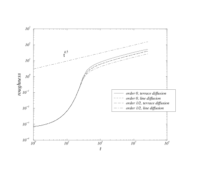
FIG. 6.: One sided case: The roughness of the meander obeys a scaling law: $w\sim t^{1/2}$.

VII Two-sided steps in phase

In the two-sided regime (i.e. $d_{+}$ and $d_{-}$ finite), a similar multi-scale analysis can be performed for in-phase steps. We find:

$$\partial_{t}\zeta=\partial_{x}\left[-{\Omega F\over 2}\partial_{x}\zeta{\ell_{\bot}^{2}(d_{-}-d_{+})\over d_{+}+d_{-}+\ell_{\bot}}+{1\over(1+(\partial_{x}\zeta)^{2})^{1/2}}\left(D_{L}a+D_{S}{\ell^{2}+\ell_{\bot}(d_{+}+d_{-})\over d_{+}+d_{-}+\ell_{\bot}}\right)\partial_{x}(\Gamma\kappa)\right].$$ (87)

Although this equation looks more complicated, the meander evolution is qualitatively similar to that found in the one-sided case (which is recovered by taking the limit $d_{-}\rightarrow\infty$ in Eq.(87)). Indeed, plateau formation and power law behavior of the roughness (with the same exponent $\sim t^{1/2}$) are also found in the two-sided case.

More details on step behavior, such as the plateau size, can be gained from the analytical investigation of Eq.(87), as shown in Appendix B. In the pure line diffusion regime $D_{L}a\gg D_{S}\ell$, we have:

$$\lambda_{0}=\lambda_{c}I(\tilde{\delta}),$$ (88)

where $\lambda_{0}/2$ is the plateau size, $\tilde{\delta}=\ell/(\ell+d_{+}+d_{-})$, and I is the same function as in Eq.(83). In the pure terrace diffusion case $D_{L}a\ll D_{S}\ell$, we find:

$$\lambda_{0}=\lambda_{c}I(1-\tilde{\delta}).$$ (89)

These result are in good agreement with numerical solution of Eq.(87) (see Fig.7).

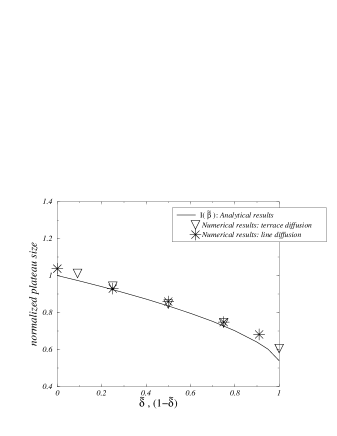
FIG. 7.: In solid line is plotted the normalized plateau size $I(\tilde{\beta})$. Symbols represent numerical results: $\bigtriangledown$ refers to the pure terrace diffusion case, and $\star$ to pure line diffusion.

VIII Discussion and summary

Starting from the BCF model, we have extracted a nonlinear evolution equation for the step meander. This equation is highly nonlinear, and thus, could not be expected from traditional phenomenological approaches, where linear terms are simply supplemented with an additive nonlinear term, as in the case of KS or KPZ equations.

A central result of the present study is that the late time power law behavior of the amplitude of the meander $w\sim t^{1/2}$ is a robust feature, regardless of the details of the evolution equation (one-sided, two-sided, line diffusion….). It is an important task for future investigations to see whether this property could be derived directly from the basic BCF equations. A second interesting point which is worth of mention is that higher order terms destroy the up-down symmetry, but the power law $w\sim t^{1/2}$ remains unaffected. The same conclusion follows from full lattice gas simulations as briefly reported in Ref.[1]. A natural question arises: could the amplitude temporal increase continue to evolve without bound in all circumstances until the surface breaks up into a lamellar-like pattern, or is there a physical mechanism, not accounted for here, leading to saturation of the amplitude? Experimental observation of this instability [18] seems to show such a saturation for the case of Cu(1,1,17), while experiments[27] on Si(001) does not reveal a hint towards a saturation. Possible candidates for amplitude saturations are (i) strong anisotropy, (ii) elastic step interactions. We hope to report along these lines in the near future.

It is worth pointing out that the use of equilibrium formula to evaluate the stabilizing line diffusion effect could be criticized, since densities of kinks and of mobile atoms along steps depend on growth conditions [28]. With regards to line mobility, our analysis allows extraction of the geometry dependence of the mobility for large meander amplitude. This treatment should serve as a basis for the nonlinear study of relaxation towards equilibrium (i.e. thermal smoothening) of large perturbations on vicinal surfaces [29].

Perhaps one of the most striking result is the manifestation of rather ’stringent’ plateaus, which are likely linked to the non-standard character of the evolution equation. It is interesting to note that the plateaus are a feature of a continuum theory, a finding which is to be compared to a long standing problem in the context of ES-induced mound formation [30]. In all previous studies, mound plateaus were indeed considered as a signature of the breakdown of continuum theories. We have shown here, in contrast, that a single equation in the continuum limit can produce such plateaus, without having resort to specific ingredients in the angular region. It is not yet clear what kind of equation in the continuum limit would describe these dynamics for mound formation. Is it similar or not to the one encountered here? These questions constitute an important line for future inquiries.

A Geometrical origin of the destabilizing term

In Eq.(74), the relaxation term is interpreted as a Cahn-Hilliard contribution. We present here a derivation of the destabilizing term from geometrical considerations in the one-sided limit.

Let us consider a curved part of the step as shown in Fig.8. In the one-sided model, step motion results from incorporation of adatoms from the terrace ahead of it. Mass conservation for an element of terrace surface $\Delta S$, hatched in Fig.8, reads:

$$v\Delta x=\Omega F\Delta S+j_{\bot}(x)-j_{\bot}(x+\Delta x)$$ (A1)

where $v$ is the step velocity along the $z$ axis, and $\Delta x$ the extent of the step element $CC^{\prime}$ along the $x$ axis. The number of atoms entering the step is $v_{n}\Delta s=v\Delta x$. $j_{\bot}(x)$ is the total flux accross the $BC$ segment in Fig.8. $\Delta S$ is written as:

$$\Delta S\approx\ell\Delta x-{\cal A}(x)+{\cal A}(x+\Delta x),$$ (A2)

where $v$ is the step velocity along the $z$ axis, and ${\cal A}(x)$, the area of the triangle $ABC$ on Fig.8, is a function of $\partial_{x}\zeta$:

$${\cal A}(x)={\ell^{2}\over 2}\cos(\theta)\sin(\theta)={\ell^{2}\over 2}\,{\partial_{x}\zeta\over 1+(\partial_{x}\zeta)^{2}}\;,$$ (A3)

where $\theta$ is the angle between the $z$ axis and the normal to the step. In the long wavelength limit, the local geometry of the terrace is completely described by $\ell_{\bot}$, the length of $BC$ on Fig.8, $\kappa$, the step curvature, and their derivatives with repect to the arclength $s$ along the steps. Since the flux $j_{\bot}$ can only come from a variation of the local geometry along $s$, we have, at most

$$j_{\bot}\sim\partial_{s}\ell_{\bot}\sim\partial_{xx}\zeta\ll{\cal A}\sim\partial_{x}\zeta\;,$$ (A4)

which shows that terms containing $j_{\bot}$ can be neglected to leading order in Eq.(A1) . Combining Eq.(A1), Eq.(A2), and (A3), and letting $\Delta x$ going to zero, we find:

$$v=\Omega F\ell-\partial_{x}\left({\Omega F\ell^{2}\over 2}{\partial_{x}\zeta\over 1+(\partial_{x}\zeta)^{2}}\right).$$ (A5)

Once the mean step velocity $V=\Omega F\ell$ is subtracted, we recover the first term of Eq.(74).

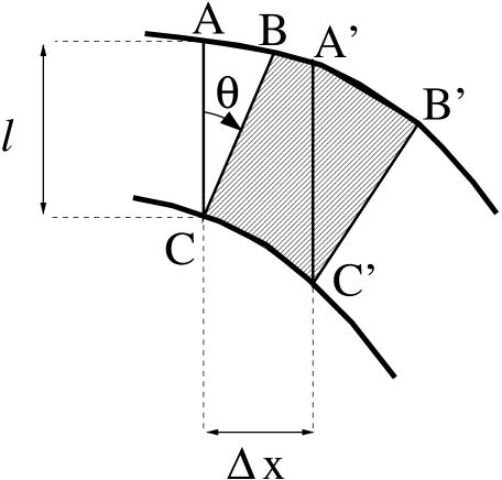
FIG. 8.: The element of terrace area $\Delta S$ that feeds one element of step, is hatched. Its area (approximated by that of BB’C’C) is the sum of $\ell\Delta x$, the area of AA’C’C, minus ${\cal A}(x)$ is the area of the triangle ABC, plus ${\cal A}(x+\Delta x)$ the area of A’B’C’.

B Late time behavior

In this appendix we derive analytically the main results obtained numerically. Despite the highly nonlinear character of the evolution equation, we show here that some simple ansatz allows to describe the asymptotic regime with good accuracy.

1 Large slope regions and extrema regions

We found the conserved evolution equation of the step meander:

$$\partial_{t}\zeta=-\partial_{x}j[\zeta],$$ (B1)

with the mass flux (see Eq.(87)):

$$j[\zeta] = {1\over(1+(\partial_{x}\zeta)^{2})^{1/2}}\left[{\alpha\,\partial_{x}\zeta\over\delta+(1+(\partial_{x}\zeta)^{2})^{1/2}}\right.$$ (B2)

$$+ \left.\left(D_{L}a+D_{S}\ell{1+\delta(1+(\partial_{x}\zeta)^{2})^{1/2}\over\delta+(1+(\partial_{x}\zeta)^{2})^{1/2}}\right)\partial_{xx}\left({\Gamma\partial_{x}\zeta\over(1+(\partial_{x}\zeta)^{2})^{1/2}}\right)\right],$$ (B3)

where $\delta=l/(d_{+}+d_{-})$, and $\alpha=\Omega F\ell^{2}(d_{-}-d_{+})/2(d_{+}+d_{-})$. For the large slope region we make use of the variable separation:

$$\zeta_{s}(x,t)=A(t)\,g(x),$$ (B4)

where $A\gg 1$, and $\partial_{x}g\neq 0$ for any value of $x$. Substituting in Eq.(B3), one finds that the destabilizing term (proportional to $\alpha$) dominates and:

$$AA^{\prime}=\alpha{g^{\prime\prime}\over gg^{\prime 2}}=C,$$ (B5)

where $C$ is a constant, and the prime stands for the derivative. The late time solution of these equations reads:

$$A = (2Ct)^{1/2}$$ (B6)

$$g = (2\alpha/C)^{1/2}{\rm erf^{-1}}(4x/\lambda_{s})\;.$$ (B7)

$\lambda_{s}$ being a constant, and erf$(x)$ the error function. Inserting these expressions in Eq.(B4), we find that the meander does not depend on $C$:

$$\zeta_{s}(x,t)=2(\alpha t)^{1/2}{\rm erf^{-1}}(4x/\lambda_{s})\;,$$ (B8)

FIG. 9.: Asymptotic meander morphology. $\lambda_{m}$ is the period of the meander and is also the most unstable wavelength obtained from linear stability analysis. $h_{0}$ is the amplitude of the meander and $\lambda_{0}/2$ is the width of a plateau. In the large slope regions (of width $\lambda_{s}/2$), the meander can be fitted by an erf like function (see Eq.(B8)). $j_{0}$ is the mass flux coming from these large slope regions toward the plateaus.

This solution describes regions of large slopes, but is not expected to accurately describe the shape around the extrema of $\zeta$ where the slope $\partial_{x}\zeta$ approaches zero. In those regions of width $\lambda_{0}/2$ and of meander amplitude of the order of $h_{0}$ (see Fig.9), global mass conservation implies:

$$2j_{0}={\lambda_{0}\over 2}\partial_{t}h_{0},$$ (B9)

where $j_{0}$ is the mass flux coming from the large slope regions. From Eq.(B3), we have:

$$j_{0}\approx{\alpha\over\partial_{x}\zeta_{s}(x_{0},t)},$$ (B10)

where $x_{0}=(\lambda_{m}-\lambda_{0})/4$ is the abscissa of the crossover point between high slope and extrema regions, and the period of the meander $\lambda_{m}$ is that of the most unstable mode obtained from linear analysis. Using $h_{0}=\zeta_{s}(x_{0},t)$ and Eq.(B8):

$${\lambda_{0}\over 4}={\lambda_{m}\over 4}-{\lambda_{s}\over 4}{\rm erf}\left[{h_{0}\over 2(\alpha t)^{1/2}}\right],$$ (B11)

so that Eq.(B9) now reads:

$${1\over t^{1/2}}\,{\alpha^{1/2}\lambda_{s}\over 4\sqrt{\pi}}\,{\rm exp}\left[-\left({h_{0}\over 2(\alpha t)^{1/2}}\right)^{2}\right]$$ (B12)

$$=\partial_{t}h_{0}\left[{\lambda_{m}\over 4}-{\lambda_{s}\over 4}{\rm erf}\left[{h_{0}\over 2(\alpha t)^{1/2}}\right]\right],$$ (B13)

This equation has the trivial solution: $h_{0}=a_{0}t^{1/2}$. Using this solution and Eq.(B11), $\lambda_{0}$ is seen not to depend on time. In the extrema region, we therefore look for solutions of the form:

$$\zeta_{p}(x,t)=B_{\pm}(t)+h(x).$$ (B14)

with $B_{\pm}(t)=\pm a_{0}t^{1/2}$, where the plus and minus signs refer to the maxima and the minima regions respectively. Upon substitution in the evolution equation (B3), we find that the problem amounts to finding the stationary solutions $\partial_{x}j[h(x)]=0$. Looking for solutions with left-right symmetry $x\rightarrow-x$ we finally have to solve

$$j[h(x)]=0.$$ (B15)

This will be exploited in the next section.

The parameters $\lambda_{s}$, $\lambda_{0}$ and $a_{0}$ are not independent. Using Eq.(B9) and Eq.(B11), we have two relations, so that $\lambda_{s}$ and $a_{0}$ can be determined as a function of $\lambda_{0}$. From Eq.(B13), we get an implicit equation for $a_{0}$:

$${\lambda_{m}\over\lambda_{0}}-1=\sqrt{\pi}\left({a_{0}\over 2\alpha^{1/2}}\right){\rm exp}\left[\left({a_{0}\over 2\alpha^{1/2}}\right)^{2}\right]{\rm erf}\left[{a_{0}\over 2\alpha^{1/2}}\right].$$ (B16)

The expression for $\lambda_{s}$ is:

$$\lambda_{s}=\lambda_{0}\sqrt{\pi}\left({a_{0}\over 2\alpha^{1/2}}\right){\rm exp}\left[\left({a_{0}\over 2\alpha^{1/2}}\right)^{2}\right].$$ (B17)

Hence, the asymptotic behavior of the meander (defined by Eq.(B8) for high slopes and Eq.(B14) for small ones) only depends on the size of the extrema region $\lambda_{0}/2$ (since the two parameters $a_{0}$ and $\lambda_{s}$ are linked to $\lambda_{0}$). How the plateau size is related to the model parameters will be considered in the next section.

2 Plateau size

In the one-sided limit we have $\delta=0$, and Eq.(B15) yields (in view of Eq.(B3)):

$$0=\alpha{h^{\prime}\over 1+h^{\prime 2}}+\left({D_{S}\ell\Gamma\over 1+h^{\prime 2}}+{D_{L}a\Gamma\over(1+h^{\prime 2})^{1/2}}\right)\partial_{xx}\left({h^{\prime}\over(1+h^{\prime 2})^{1/2}}\right).$$ (B18)

Introducing the abbreviation:

$$m={h^{\prime}\over(1+h^{\prime 2})^{1/2}},$$ (B19)

we can rewrite it in a familiar form:

$$\left({(D_{S}\ell+D_{L}a)\Gamma\over\alpha}\right)m"=-{m\over\tilde{\beta}(1-m^{2})^{1/2}+(1-\tilde{\beta})}=-{dU\over dm},$$ (B20)

analogous to that describing the motion of a particle of position $m$ as a function of time $x$ in a potential $U$. We have defined $\tilde{\beta}=D_{S}\ell/(D_{S}\ell+D_{L}a)$, and:

$$U(m)=\int_{0}^{m}{m\,dm\over\tilde{\beta}(1-m^{2})^{1/2}+(1-\tilde{\beta})}.$$ (B21)

Multiplying Eq.(B20) by $m^{\prime}$ and integrating with respect to $x$, we get the analogue of the ”energy conservation” condition:

$${1\over 2}\left({(D_{S}\ell+D_{L}a)\Gamma\over\alpha}\right)m^{\prime 2}+U(m)=U(m_{0}),$$ (B22)

where $m_{0}$ is the turning point (i.e. $m^{\prime}=0$ when $m=m_{0}$). We look for solutions having two ”vertical” tangents where the step slope diverges: $\partial_{x}\zeta\rightarrow\pm\infty$, (i.e. $m_{0}\rightarrow\pm 1$) in order to match the extrema solution with the large slope region. The size of the extrema region reads:

$${\lambda_{0}\over 2}=\int_{0}^{\lambda_{0}/2}dx=\int^{m_{0}}_{-m_{0}}{dm\over m^{\prime}},$$ (B23)

where $m_{0}\rightarrow 1$. Using Eq.(B22), we find:

$${\lambda_{0}\over\lambda_{m}}={I(\tilde{\beta})\over\sqrt{2}},$$ (B24)

where

$$\lambda_{m}=2\pi\left(2{(D_{S}\ell+D_{L}a)\Gamma\over\alpha}\right)^{1/2}$$ (B25)

is the the wavelength of the most unstable mode obtained from linear analysis, and

$$I(\tilde{\beta})={1\over\pi\sqrt{2}}\int_{-1}^{1}{dm\over[U(1)-U(m)]^{1/2}}$$ (B26)

is plotted in Fig.4. $I(\tilde{\beta})$ is a decreasing function with $I(0)=1$ and $I(1)\approx 0.54$. Hence the extrema region size is finite and always smaller than $\lambda_{c}=\lambda_{m}/\sqrt{2}$.

The meander variation in this region, as compared to the total amplitude of the meander, decreases as $t^{-1/2}$, and the step looks as if plateaus were present.

The reader is invited to repeat the calculation in the two-sided case –where $\delta$ is finite, in presence of pure line ($\tilde{\beta}=0$) or terrace diffusion ($\tilde{\beta}=1$). Surprisingly, the same integral $I$ appears. Let us define $\tilde{\delta}=\ell/(\ell+d_{+}+d_{-})$. We find in the pure line diffusion case:

$${\lambda_{0}\over\lambda_{m}}={I(\tilde{\delta})\over\sqrt{2}},$$ (B27)

and in the pure terrace diffusion case:

$${\lambda_{0}\over\lambda_{m}}={I(1-\tilde{\delta})\over\sqrt{2}}.$$ (B28)

Hence, $\lambda$ never exceeds $\lambda_{m}/\sqrt{2}=\lambda_{c}$ the largest wavelength for which the meander is linearly stable.

We can use a similar treatment to analyze the case with higher order terms (eq.84). The main point is that terms proportional to $\epsilon^{1/2}$ do not affect the long time behaviour obtained from the ansatz B4). Consequently, in large slope regions, we expect once again $\zeta\sim t^{1/2}$. Terms breaking the front-back symmetry will affect differently maxima and minima regions, as seen in Fig.5, because the effective potential $U(m)$ is not invariant under the $m\rightarrow-m$ transformation anymore, which corresponds to the up-down $z\rightarrow-z$ for step meander. We shall not develop here further this point; for more details see[26].

The numerical solution of Eq.(B1) is performed in order to check the validity of the analytical results. First, the qualitative profile of the meander is in good agreement with the above description. We found the predicted scaling of the amplitude of the meander $\sim t^{1/2}$ in all simulations performed so far, expect in the case of very small kinetic lengths $(d_{+}+d_{-})/l<10^{-2}$, where we were not able to explore the late time behavior, due to bad numerical convergence.

As shown in Fig. 4 and 7, the observed plateau size, is in very good agreement with the prediction of Eq.(B24, B28,B27).

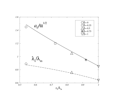
FIG. 10.: The solid line represents the prediction for the amplitude $a_{0}$ as a function of $x_{0}/\lambda_{m}$. The dashed curve is the prediction of the dimensionless ratio $\lambda_{s}/\lambda_{m}$. Symbols represent data from numerical solution of Eq. (64) (the one-sided case), as $\tilde{\beta}$ is varied.

The value of $a_{0}$ is extracted from the evolution of the meander amplitude via the relation:

$$\zeta_{p,max}-\zeta_{p,min}\approx 2a_{0}t^{1/2}.$$ (B29)

$\lambda_{s}$ is calculated from a fit of $\partial_{x}\zeta$ at $\zeta=0$:

$$\partial_{x}\zeta_{s}|_{\zeta=0}={4\sqrt{\pi}\over\lambda_{s}}(\alpha t)^{1/2}.$$ (B30)

In Fig.10, both numerical values are compared to the prediction of Eq.(B16) in the one-sided limit, where $\lambda_{0}$ is calculated from Eq.(B24). Once again, good agreement is found.

REFERENCES

- [1] O. Pierre-Louis et al., Phys. Rev. Lett. 80, 4221 (1998).
- [2] J. Villain, J. Phys. France I 1, 19 (1991).
- [3] O. Pierre-Louis and C. Misbah, Phys. Rev. B 58, 2276 (1998).
- [4] M. Kardar, G. Parisi, and Y. C. Zhang, Phys. Rev. Lett. 56, 889 (1986).
- [5] I. Bena, C. Misbah, and A. Valance, Phys. Rev. B 47, 7408 (1993).
- [6] O. Pierre-Louis and C. Misbah, Phys. Rev. Lett. 76, 4761 (1996).
- [7] G. S. Bales and A. Zangwill, Phys. Rev. B 41, 5500 (1990).
- [8] W. K. Burton, N. Cabrera, and F. C. Frank, Phil. Trans. Roy. Soc. London, A, 243, 299 (1951).
- [9] R. L. Schwoebel, J. Appl. Phys. 40, 614 (1969).
- [10] T. Ihle, C. Misbah, and O. Pierre-Louis, Phys. Rev. B 58, 2289 (1998).
- [11] F. Gillet and C. Misbah (unpublished).
- [12] O. Pierre-Louis and C. Misbah, Phys. Rev. B 58, 2259 (1998).
- [13] W. W. Mullins, J. Appl. Phys. 28, 333 (1957).
- [14] J. Villain and A. Pimpinelli, Physique de la croissance cristalline (Eyrolles Alea Saclay, Paris, 1995).
- [15] M. Giessen-Seibert, R. Jentjens, M. Poensgen, and H. Ibach, Phys. Rev. Lett. 71, 3521 (1993).
- [16] M. Giesen-Seibert, F. Schmitz, R. Jentjens, and H. Ibach, Surf. Scie. 329, 47 (1993).
- [17] A. Pimpinelli et al., J. of Physic 6, 2661 (1994).
- [18] T. Maroutian, L. Douillard, and H. J. Ernst, Phys. Rev. Lett. 83, 4353 (1999).
- [19] P. Stoltze, Phys. Condens. Matter 6, 9495 (1994).
- [20] J. Cahn and J. E. Hilliard, J. Chem. Phys. 28, 258 (1958).
- [21] P. C. Hohenberg and B. I. Halperin, Rev. Mod. Phys. 49, 435 (1977).
- [22] M. Kadar, G. Parisi, and Y. C. Zhang, Phys. Rev. Lett. 56, 889 (1986).
- [23] S. A. Langer, R. E. Goldstein, and D. P. Jackson, Phys. Rev. A 46, 4894 (1992).
- [24] Z. Csahók, C. Misbah, and A. Valance, Physica D 128, 87 (1999).
- [25] J. Kallunki and J. Krug independently curred the same problem and found plateau-like structures by numerically integrating Eq.(74); private communication.
- [26] F. Gillet, Ph.D. thesis, Thèse de doctorat de l’université Grenoble I, Grenoble, 2000.
- [27] F. Wu, S. Jaloviar, D. Savage, and M. Lagally, Phys. Rev. Lett. 71, 4190 (1993).
- [28] O. Pierre-Louis, M. R. D’Orsogna, and T. L. Einstein, Phys. Rev. Lett. 82, 3661 (1999).
- [29] H.P. Bonzel and W.W. Mullins, SS 350, 285 (1996).
- [30] J. Tersoff, A. W. D. van der Gon, and R. M. Tromp, Phys. Rev. Lett. 72, 266 (1994); J. Krug, P. Politi, and T. Michely, preprint, cond-matt.