Four-wave mixing in degenerate atomic gases

Abstract

We study the process of four-wave mixing (4WM) in ultracold degenerate atomic gases. In particular we address the problem of 4WM in boson-fermion mixtures. We develop an approximate description of such processes using asymptotic analysis of high order perturbation theory taking into account quantum statistics. We perform also numerical simulations of 4WM in boson-fermion mixtures and obtain an analytic and numerical estimate of the efficiency of the process.

In the recent years atom optics has become a flourishing subject. With the successful experiments on Bose-Einstein condensation [1, 2, 3] new possibilities to study linear[4] and nonlinear atom-optics[5] with macroscopic wave packets have emerged. So far, the most spectacular experiment in nonlinear atom optics concerns the observation of the so called four-wave mixing of bosonic matter waves[6]. In this nonlinear process, three macroscopic matter wave packets interact and produce a fourth one. Also recently, Jin et al. [7] have managed to trap and cool a sample of spin polarized ⁴⁰K below the Fermi temperature in a harmonic trap. This has triggered an outburst of activities in trying to understand the properties of ultracold fermionic systems[8], and has stimulated a great interest in the studies of fermion-boson mixtures[9]. In particular, the question “is non-linear atom optics with fermions possible?” has been posed[10].

In this Letter we investigate the process of four-wave mixing (4WM) in fermion-boson mixtures and demonstrate that under an appropriate choice of parameters it is possible to create a macroscopic fourth wave of fermions. The recent experiment of Deng et al. [6] with Bose-Einstein condensates have demonstrated that 4WM in bosonic gases is a truly macroscopic process with an efficiency of the order of $6\%$. In this experiment Bragg pulses [11] were used to create three condensate clouds, which then interacted through collisions. Four wave mixing of matter waves can also be described – using the language of optics – as Bragg scattering from a grating. In this picture, two counter propagating condensates create the grating from which the third condensate scatters, generating a fourth one.

An intuitive understanding of Bragg scattering for bosons may be obtained considering a homogeneous condensate in a box of volume $V$. For such a case, the Hamiltonian has the form:

$$\hat{H}=\sum_{\vec{k}}\epsilon_{\vec{k}}a^{{\dagger}}_{\vec{k}}a_{\vec{k}}+{1\over 2}u_{0}\sum_{\vec{k},\vec{k}^{\prime},\vec{q}}a^{{\dagger}}_{\vec{k}+\vec{q}}a^{{\dagger}}_{\vec{k}^{\prime}-\vec{q}}a_{\vec{k}^{\prime}}a_{\vec{k}},$$ (1)

where $u_{0}=\frac{4\pi\hbar^{2}a}{mV}$ is the interaction strength proportional to the $s$-wave scattering length $a$ and $\epsilon_{\vec{k}}$ is the kinetic energy. Let us consider as an initial state $|i\rangle=|N_{1},\vec{k}_{1};N_{2},\vec{k}_{2};N_{3},\vec{k}_{3}\rangle$ representing $N_{i}$ particles of momentum $\vec{k}_{i}$, $i=1,2,3$. Assume for the moment that only one particle is scattered leading to the final state $|f\rangle=|N_{1}^{\prime},\vec{k}_{1};N_{2}^{\prime},\vec{k}_{2};N_{3}^{\prime},\vec{k}_{3};1,\vec{k}_{4}\rangle$ with $\vec{k}_{4}\neq\vec{k}_{i}$ for $i=1,2,3$. Among all the processes which conserve momentum and energy the one corresponding to

$$\vec{k}_{4}=\vec{k}_{1}-\vec{k}_{2}+\vec{k}_{3}$$ (2)

is particularly favorable and represents in fact the first order Bragg scattering [12, 13] (see Fig. 1). The above process corresponds to the term $a_{\vec{k}_{4}}^{\dagger}a_{\vec{k}_{2}}^{\dagger}a_{\vec{k}_{1}}a_{\vec{k}_{3}}$ in the Hamiltonian. This term accounts for the creation of a particle in the “grating state” $\vec{k}_{2}$ which is already macroscopically occupied. This leads to the appearance of a bosonic enhancement factor $\sqrt{N_{2}+1}$ in the transition amplitude associated with the process $|i\rangle\rightarrow|f\rangle$. From this point of view, due to bosonic enhancement Bragg scattering is the most probable process.

Let us extend the previous analysis to the case where many particles are scattered. Clearly, the most probable final state is of the form $|f\rangle=|N_{1}^{\prime},\vec{k}_{1};N_{2}^{\prime},\vec{k}_{2};N_{3}^{\prime},\vec{k}_{3};N_{4},\vec{k}_{4}\rangle$, where $\vec{k}_{4}$ is given by Eq.(2). This final state must respect the conservation of momentum

$$\sum_{i=1}^{3}N_{i}\vec{k}_{i}=\sum_{i=1}^{3}N_{i}^{\prime}\vec{k}_{i}+N_{4}\vec{k}_{4}\,,$$ (3)

and the conservation of the particle number

$$\sum_{i=1}^{3}N_{i}=\sum_{i=1}^{3}N_{i}^{\prime}+N_{4}\,.$$ (4)

Eqs.(2),(3) and (4) imply conservation of energy. In the reference frame in which $\vec{k}_{1}$ and $\vec{k}_{2}$ are collinear the scattering process is planar. Thus we have five equations with six unknown parameters $N^{\prime}_{i},N_{4},\vec{k}_{4}$. The actual value of $N_{4}$ can be determined by maximizing the transition probability $P_{if}$. Using perturbation theory with respect to the off-diagonal elements of the Hamiltonian in Eq.1, we calculate the transition amplitude $T_{if}$. For $N_{1}=N_{2}=N_{3}$ this quantity exhibits a divergence for $\eta=N_{4}/N_{tot}=1/6\approx 16.7\%$, where $N_{tot}$ is the total number of particles. This divergence appears due to the simplicity of the model and can be removed by using wave packets instead of plane waves. In any case, $P_{if}$ will be strongly peaked at $N_{4}\sim N_{tot}/6$. We expect that the actual efficiency of the process – which in principle has to be calculated non perturbatively – will be of the same order of magnitude. Furthermore, our analysis predicts a saturation of the efficiency with increasing number of atoms, which can be understood as a consequence of the Bose statistics. These results are in agreement with the experimental results of Ref. [6].

We turn now to the case of fermions. The previous analysis clearly stresses the role of bosonic enhancement; the macroscopic occupation of the states that form the grating select Bragg scattering as the most favorable process. From this point of view, the use of a fermionic grating would lead to a rather poor Bragg scattering. For this reason we consider Bragg scattering of an incoming cloud of fermions on a bosonic grating. In our model, fermions and bosons interact via two-body $s$-wave scattering. The incoming fermions must obey momentum and energy conservation as in the case of boson-boson scattering. For fermions there will be inevitably a momentum spread due to Fermi statistics. In order to fulfill the Bragg condition, illustrated in Fig. 1, the momentum spread in the fermionic sample $\Delta k$, must be restricted to $\Delta k\ll|\vec{k}_{1}-\vec{k}_{2}|$. This condition can be achieved by trapping the fermions initially in a sufficiently shallow trap which results in a well localized momentum distribution.

Solving the complete many-body scattering problem for the fermions is a formidable task. In our case we can simplify the situation assuming first that the fermions do not interact. This is a good approximation as long as we consider a polarized Fermi gas. The interaction of fermions of only one specie is entirely due to $p$-wave scattering which is negligible at very low temperatures [14]. Second, we model the bosonic grating by a scalar potential proportional to the local condensate density. In doing this we sacrifice in some sense the effects of the statistics. In fact, the Fermi statistics appears in our model only through the preparation of the initial state, which must obey Pauli principle. We also neglect any back-action from the fermions on the bosons. This last approximation is valid in a situation where the boson density is much larger than the fermion density. Finally, since the dynamics is basically two dimensional (see Fig. 1) we restrict our numerical simulations to 2D. With these assumptions we solve the Schrödinger equation for the fermions with an effective external potential of the form:

$$V_{f}(x,y)=u_{BF}n_{b}(x,y)\,,$$ (5)

with $u_{BF}={{8\pi\hbar^{2}a}\over{mL}}$. Here $a$ denotes the fermion–boson $s$-wave scattering length, $m$ the (same) mass for both fermions and bosons, $L$ the thickness of the cloud in $z$-direction, whereas $n_{b}(x,y)$ the equilibrium density of the condensate. For the bosons, the trap potential is a combination of a harmonic potential in the y-direction and a periodic structure in x-direction created for instance by a standing-wave laser,

$$V_{b}(x,y)={1\over 2}m\Omega_{c}^{2}y^{2}+U_{l}\cos^{2}(|\vec{k}_{1}-\vec{k}_{2}|x).$$ (6)

We have solved numerically the Gross-Pitaevskii equation with the potential in Eq. 6, in order to determine the equilibrium bosonic density $n_{b}(x,y)$, which, in turn, results in a periodic potential $V_{f}(x,y)$ for the fermions. The back action of fermions on bosons can be neglected provided $u_{BF}n_{f}(x,y)/\mu\ll 1$ where $\mu$ is the chemical potential of the trapped condensate and $n_{f}(x,y)$ the fermion density. In our simulation this ratio was kept smaller than 0.01.

Our procedure is now as follows: initially the fermions are trapped in a 2D potential of the form $V(x,y)=m\Omega^{2}(x^{2}+y^{2})$ centered at $(x_{0},y_{0})$. The number of fermions is such that the Fermi level still fulfills the condition $k_{F}\ll|\vec{k}_{1}-\vec{k}_{2}|$. The trap is then removed and a momentum kick $\hbar{\vec{k}_{3}}$ is given to the fermions by illuminating the sample with a detuned laser propagating in the direction of $\vec{k}_{3}$ [6, 15] so the fermion cloud scatters from the grating. We finally monitor the density of fermions to obtain the efficiency of the process.

The wave functions of the non interacting fermions fulfill all the same Schrödinger equation

$$i\hbar{\partial\over{\partial t}}\Psi_{i}=\left[-{{\hbar^{2}}\over{2m}}\nabla_{i}^{2}+V_{f}(x,y)\right]\Psi_{i},i=1,...,N_{3},$$ (7)

but with different initial conditions for each fermion. The initial states are the eigenstates of the displaced harmonic potential used for trapping the fermions,

$$\Psi_{n_{x},n_{y}}(x,y)=A_{n_{x},n_{y}}e^{i\vec{k}_{3}\cdot\vec{x}}e^{-{1\over 2}(\tilde{x}^{2}+\tilde{y}^{2})}H_{n_{x}}(\tilde{x})H_{n_{y}}(\tilde{y}),$$ (8)

where $\tilde{x}=(x-x_{0})/\sqrt{\hbar/m\Omega}$ and $\tilde{y}=(y-y_{0})/\sqrt{\hbar/m\Omega}$, $H_{n_{x}}$ denotes the Hermite polynomials and $A_{n_{x},n_{y}}$ is the normalization constant.

The scattering of the fermions can now be numerically simulated one by one. We monitor the density in the region where the Bragg scattered fermions are supposed to appear. In our model, for the fermion cloud we use ⁴⁰K atoms and a trap frequency of $\Omega/2\pi=10$ Hz while for the bosonic trap we use a frequency of $\Omega_{c}=40\Omega$. This produces a narrow grating compared to the size of the fermionic cloud. Furthermore, we have taken the scattering length value as $a=6.0$ nm and $L=30$ $\mu$m with $N_{c}=2\cdot 10^{5}$ bosons in the condensate. The grating has an associate wave number of $k_{1}=1.3$ $\mu$m^-1 ($\vec{k}_{1}=-\vec{k}_{2}$) and $k_{F}/k_{1}<0.7$. The initial fermion cloud is positioned at $x_{0}=y_{0}=-40$ $\mu$m and the momentum kick is settled to $\vec{k}_{3}=(1.3,1.3)\mu$m^-1.

In Fig.2 we show the efficiency $\eta=N_{4}/N_{3}$ of the Bragg process as a function of the total number of fermions $N_{3}$. With an increasing number of particles ($N_{3}$) the efficiency decreases due to the increase of the momentum spread of the fermions. Fig. 3 displays a snapshot of the cloud after the scattering. We observe that approximately 3% of the cloud is scattered in the Bragg direction. In this figure one can also see that a part of the fermionic cloud is reflected due to the chosen relation between the incoming fermion kinetic energy and the contrast together with the maximum of the grating potential. Note also the appearance of the reflected wave packet in the direction $-\vec{k}_{3}$ which in fact corresponds to a Bragg reflection. Reflections are drastically reduced if the scattering length is negative since in this case the potential $V_{f}(x,y)$ becomes attractive. The Bragg scattering relies on the periodicity and contrast of the grating and it is present for both positive and negative scattering lengths. Also, for a fixed interaction time the efficiency of the Bragg process decreases with the contrast of the grating.

In order to understand the above results we have developed an approach similar to the one used for bosons, based on perturbative analysis using plane waves. We want to study the efficiency of the process starting with the fermionic state $|i\rangle=|1,{\vec{k}_{3}}+{\vec{\chi}_{1}};...;1,{\vec{k}_{3}}+{\vec{\chi}_{N_{3}}}\rangle$ and considering a generic final state in which $N_{4}$ holes are created in the Fermi sea of states with momentum close to $\vec{k}_{3}$. There are $j={N_{3}\choose N_{4}}$ different orthogonal final states $|f_{j}\rangle$. In order to simplify the problem we assume that the transition amplitude does not depend strongly on $|f_{j}\rangle$, which is a valid assumption as long as $\Delta k\ll|\vec{k}_{1}-\vec{k}_{2}|$. We can then evaluate the probability $P(N_{4})$ of scattering $N_{4}$ particles by taking an average value of the transition amplitude so that $P(N_{4})\approx{N_{3}\choose N_{4}}{|\bar{T}_{if_{j}}|^{2}}$. The mean efficiency of the process defined as $\eta=\langle N_{4}\rangle/N_{3}$ is calculated then using the previous probability distribution $P(N_{4})$. We stress that the aim of this calculation is not to obtain an exact expression for the efficiency, but rather to estimate whether the scattering process can change macroscopically a many particle fermionic state.

We begin by calculating the transition amplitude $T_{if_{1}}$ between the initial state $|i\rangle$ and the final state $|f_{1}\rangle$ which corresponds to depletion of the first $N_{4}$ states of the Fermi sea around $\vec{k}_{3}$. The macroscopically populated states of the bosonic grating provide a bosonic enhancement factor $\sqrt{(N_{2}+p)}$ $(p=1,2,...,N_{4})$. Using a time dependent perturbative method [16] one obtains

$$T_{if_{1}}\propto U_{BF}^{N_{4}}\frac{\Gamma}{(E_{i}-E_{N_{4}})...(E_{i}-E_{1})},$$ (9)

where the bosonic enhancement amounts to

$$\Gamma=\frac{\sqrt{N_{1}!}\sqrt{(N_{2}+N_{4})!}}{\sqrt{(N_{1}-N_{4})!}\sqrt{N_{2}!}}.$$ (10)

The energies of the intermediate states (corresponding to the scattering of $p$-fermions) are given by

$$E_{p}=E_{B}+\frac{\hbar^{2}}{2m}\left\{\sum_{j=p+1}^{N_{3}}({\vec{k}_{3}}+{\vec{\chi}_{j}})^{2}+\sum_{j=1}^{p}({\vec{k}_{4}}+\vec{\chi}_{j})^{2}\right\}$$ (11)

with $U_{BF}=\frac{8\pi\hbar^{2}a}{mV}$, $E_{i}=E_{p=0}$ and ${\vec{k}_{2}}=k_{2}\hat{e}_{x}=-k_{1}\hat{e}_{x}$. We denote by $E_{B}$ the energy of the bosons which is constant during the process. This $T_{if_{1}}$ is the transition amplitude corresponding to one of the $N_{4}!$ possible paths going from $|i\rangle$ to $|f_{1}\rangle$. Hence there are $N_{4}!$ different $T_{if_{1}}$’s and we estimate their contribution by taking an average value. To this aim we consider the $\vec{\chi}$ ’s as independent random variables distributed between $-k_{F}$ and $k_{F}$ with a flat probability distribution $\propto\theta(k_{F}-\chi)$. Neglecting correlations between different $\vec{\chi}$ ’s is a valid approximation if $N_{4}\ll N_{3}$. Consequently we consider this regime in the following, and restrict ourselves to the values of $N_{4}\leq 0.1N_{3}$. The resulting probability of having $N_{4}$ Bragg scattered fermions is

$$P(N_{4})\propto\left(\frac{1}{\alpha^{2}}\right)^{N_{3}-N_{4}}\frac{1}{(N_{3}-N_{4})!},$$ (12)

where we have assumed $N_{1}=N_{2}$. This Poissonian probability distribution depends on the number of fermions $N_{3}$ and on the parameter

$$\alpha=\frac{2\sqrt{10}\,\pi\,a\,n_{b}}{k_{2}k_{F}},$$ (13)

which is also $N_{3}$-dependent through the dependence on the Fermi momentum $k_{F}$. The parameter $\alpha$ contains also the boson density $n_{b}$. In Fig. 4 we display the efficiency $\eta$, (defined as the mean value of $N_{4}$ over $N_{3}$) as a function of $N_{3}$ and the $N_{3}$–independent parameter $\alpha N_{3}^{1/3}$. We observe that for small values of $\alpha$ the efficiency decreases with increasing $N_{3}$. On the contrary, with larger $\alpha$ the efficiency can reach larger values, only limited by the assumptions of the model. i.e $\eta\leq 0.1$.

In summary, we have discussed the effects of Bose and Fermi statistics on four-wave mixing processes. For a pure bosonic process the Bose statistics sets a fundamental limit in the efficiency. In the case of an incoming fermionic cloud, the result depends strongly on the values of the various physical parameters involved in the problem. On one hand, we have performed a numerical analysis which shows that the momentum spread $\Delta k\ll|\vec{k}_{1}-\vec{k}_{2}|$ is a crucial parameter in order to obtain a macroscopic fourth wave. On the other hand, the analytical treatment which assumes that Bragg condition is always fulfilled, exhibits an interplay between the statistical and collisional effects leading to a decreasing efficiency for small $N_{3}$ and increasing efficiency for large $N_{3}$. Typically, for small $\alpha$, the value of $\langle N_{4}\rangle$ is negligible meaning a small efficiency. On the contrary, for sufficiently big values of $\alpha$, the efficiency is only limited by the assumptions of the model, namely the lack of correlations between the scattered particles. The efficiency can then reach values of the order of a few percent which characterizes the creation of a macroscopic fermionic fourth wave.

The authors wish to thank W. Ketterle for helpful discussions. We acknowledge support from Deutsche Forschungsgemeinschaft (SFB 407) and the TMR network ERBXTCT96-0002.

FIG. 1.: In the reference frame in which $\vec{k}_{1}$ and $\vec{k}_{2}$ are collinear the scattering process can always be described in a plane. The criterion $\vec{k}_{4}=\vec{k}_{1}-\vec{k}_{2}+\vec{k}_{3}$ together with the conservation of energy $|\vec{k}_{4}|=|\vec{k}_{3}|$ gives the Bragg condition ${k_{3}}_{x}=k_{1}$ with $\vec{k}_{1}=-\vec{k}_{2}$ chosen in the direction of the x-axis.

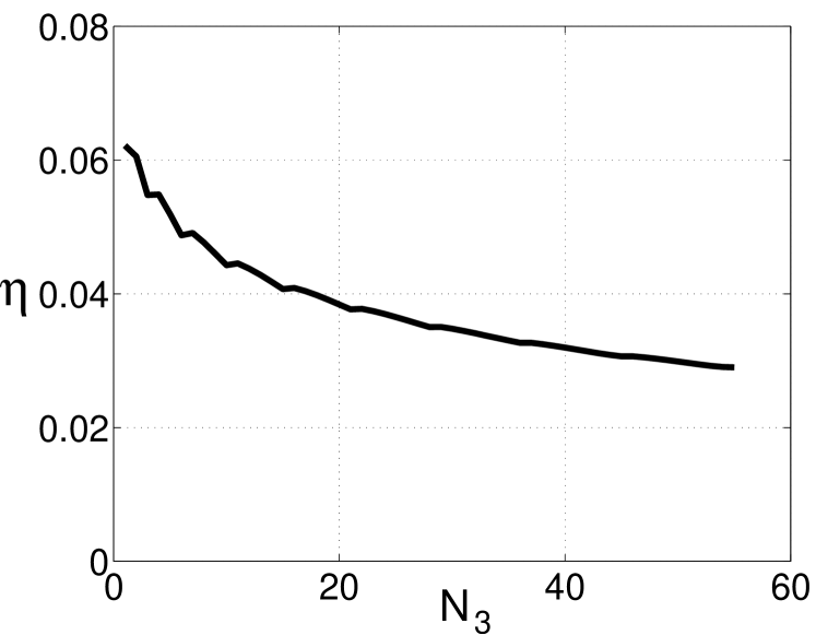
FIG. 2.: Numerical estimate of the efficiency $\eta$ of the 4WM versus the number of incoming fermions $N_{3}$. $\eta$ decreases for larger values of $N_{3}$ due to the spread of the momentum for the incoming fermions.

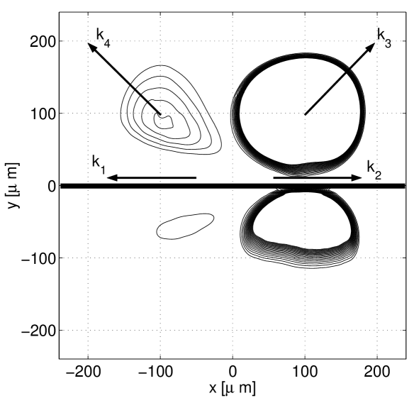
FIG. 3.: A Snapshot of the density of the fermionic cloud after the scattering. In this case $3\%$ of the atoms are found in the Bragg direction. The grating is represented by the two counter propagating waves $\vec{k}_{1}=-\vec{k}_{2}$

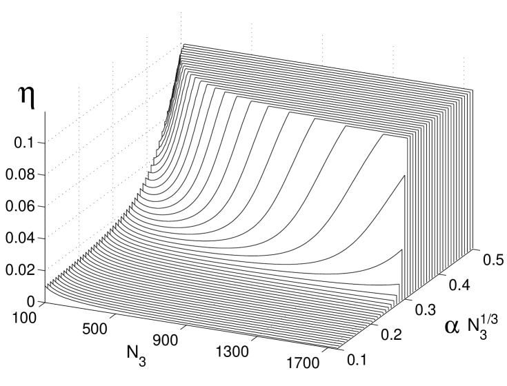
FIG. 4.: Analytical estimate of the Bragg process efficiency. The model is limited by the assumption $\eta\ll 1$. For small values of $\alpha$ the efficiency decreases with increasing $N_{3}$.

REFERENCES

- [1] M.H. Anderson et al., Science 269, 198 (1995)
- [2] K.B. Davis et al., Phys. Rev. Lett., 75, 3969 (1995)
- [3] C.C. Bradley et al., Phys. Rev. Lett. 75, 1687 (1995)
- [4] K. Bongs et al., Phys. Rev. Lett. 83, 3577 (1999)
- [5] G. Lenz, P. Meystre, and E.W. Wright, Phys. Rev. Lett. 71, 3271 (1993)
- [6] L. Deng et al., Nature 398, 218 (1999)
- [7] B. DeMarco and D.S. Jin, Science 285, 1703 (1999)
- [8] M.A. Baranov, D. S. Petrov. cond-mat/9901108; L. Vichi and S. Stringari, Phys. Rev. A, 60, 4734 (1999), H.T.C. Stoof and M. Houbiers, Proceedings of the International School of Physics “Enrico Fermi” Course CXL, eds. M. Inguscio, S. Stringari, and C.E. Wieman (IOP press Amsterdam 1999).
- [9] N. Nygaard, K. Moelmer, Phys. Rev. A, 59, 2974 (1999)
- [10] W. Phillips, private communication.
- [11] M. Kozuma et al., Phys. Rev. Lett. 82, 871 (1999)
- [12] M. Trippenbach, Y.B. Band, and P.S. Julienne, Optics Express 3, 530 (1998)
- [13] M. Trippenbach, Y.B. Band, and P.S. Julienne, cond-mat/0002119
- [14] B. DeMarco et al., Phys. Rev. Lett. 82, 4208 (1999)
- [15] S. Inouye et al., Science 285, 571 (1999)
- [16] L.D. Landau and E.M. Lifshitz, Quantum Mechanics (Pergamon Press, London-Paris, 1958)