Liquid Limits: The Glass Transition and Liquid-Gas Spinodal Boundaries of Metastable Liquids

Abstract

The liquid-gas spinodal and the glass transition define ultimate boundaries beyond which substances cannot exist as (stable or metastable) liquids. The relation between these limits is analyzed via computer simulations of a model liquid. The results obtained indicate that the liquid - gas spinodal and the glass transition lines intersect at a finite temperature, implying a glass - gas mechanical instability locus at low temperatures. The glass transition lines obtained by thermodynamic and dynamic criteria agree very well with each other.

Substances can exist in the liquid state beyond equilibrium phase boundaries in a metastable state, if nucleation of the stable phase is avoided. Such metastable liquids are nevertheless bounded by ultimate limits in the form of the liquid-gas spinodal and the glass transition locus. The liquid-gas spinodal is a limit of stability, beyond which the system is mechanically unstable. Although the nature of the glass transition, in particular the existence of an ideal glass transition, is still a matter of debate[2], the locus of glass transition temperatures defines a boundary beyond which substances transform to an amorphous solid state, and can no longer exist as liquids. A preliminary report of investigations concerning the relationship between these two limits of the liquid state are presented in this letter.

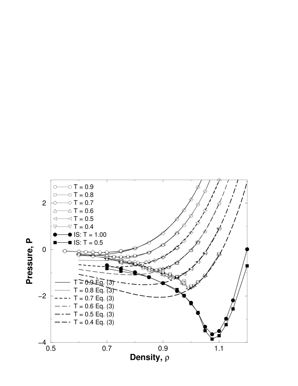
FIG. 1.: (a) Isotherms from REMC simulations (points connected with lines). (b) Curves marked ‘IS:’ are pressure vs. density curves for inherent structures, with starting temperatures $T=1.0,0.5$. (c) Continuous curves labeled ‘Eq. (3)’ are from the empirical equation of state described in the text.

The immediate motivation for the present study are observations made in Ref. [3], where a threshold density $\rho^{*}=0.89$ was identified for a model (mono) atomic liquid, across which the structure of typical local potential energy minima or ‘inherent structures’ (IS) undergoes a qualitative change from spatially heterogeneous (below $\rho^{*}$) to homogeneous structures (above $\rho^{*}$). At the same density $\rho^{*}$, the pressure $P$ vs. density curve for the inherent structures goes through a minimum. Two speculations were made in [3], motivated by these observations: (1) The threshold density $\rho^{*}$ is (or closely approximates) the $T\rightarrow 0$ limit of the liquid-gas spinodal locus $\rho_{s}(T)$, and (2) The threshold density $\rho^{*}$ forms the absolute lower density limit to glass formation. In the simplest scenario, the glass transition temperature approaches zero as $\rho\rightarrow\rho^{*}$ from above. These speculations are tested here via computer simulations of a model liquid. The results obtained also prove valuable in assessing recent approaches to studying the glass transition.

The model studied is a binary mixture of $204$ type $A$ and $52$ type $B$ particles, interacting via the Lennard-Jones (LJ) potential, with parameters $\epsilon_{AB}/\epsilon_{AA}=1.5$, $\epsilon_{BB}/\epsilon_{AA}=0.5$, $\sigma_{AB}/\sigma_{AA}=0.8$, and $\sigma_{BB}/\sigma_{AA}=0.88$, and $m_{B}/m_{A}=1$. This system has been extensively studied as a model glass former[4, 5, 6, 7]. Monte Carlo (MC) simulations in the restricted ensemble (REMC) were performed (details below) for $8$ temperatures for an average of $10$ densities, for three different sets of constraints in each case, to locate the liquid-gas spinodal locus. Run lengths ranged from $3\times 10^{5}$ to $1.8\times 10^{6}$ MC cycles. Molecular Dynamics (MD) simulations (details as in [5]) were performed at $7$ densities, $\rho=1.08,1.1,1.125,1.15,1.2,1.25,1.35$, over a wide range of temperatures (from $T=3.0$ to $0.259$ for $\rho=1.08$). Run lengths ranged from $2\times 10^{5}$ for $T>1.0$ to $6.2\times 10^{7}$ time steps (or $1.86\times 10^{5}$ LJ time units, or $0.4~{}\mu s$ in Argon units). Simulations above $T=1.0$ were typically done at constant temperature (NVT) and those below $T=1.0$ at constant energy (NVE). NVT simulations were also performed for lower densities ($\rho=0.55$ to $1.05$, for $T=1.0$ to $0.325$) to obtain isothermal compressibilities, $k_{T}$.

The liquid-gas spinodal is estimated via restricted ensemble simulations[8, 9], wherein the system is divided into cells and fluctuations in density in each cell are restricted. Isotherms so obtained display a van der Waals-type loop, and permit estimation of the spinodal density from the location of their minima (See [9] for further details)[10]. The resulting isotherms are displayed in Fig. 1, along with the $P$ vs. $\rho$ curves for inherent structures, obtained at two temperatures. The latter show that IS properties depend on the starting $T$, but the density at the minimum is not significantly altered, and is $\rho^{*}=1.08$. Finite $T$ isotherms do not show significant dependence on constraint strength. Spinodal densities $\rho_{s}(T)$ obtained from the location of minima along these isotherms, for each constraint strength, are shown (as spinodal temperatures $T_{s}(rho)$) in Fig. 2. Also shown is $\rho^{*}$ where the IS pressure is minimum. To confirm the reliability of the REMC estimates, the spinodal is also estimated (a) by fitting isotherms ($P$ vs. $\rho$) by (cubic) polynomials, and (b) by calculating $k_{T}$ directly in MD simulations, and locating the density where $k_{T}^{-1}$ vanishes by polynomial extrapolation. The results are shown in Fig. 2, which shows that spinodal densities so obtained agree well with the REMC estimates.

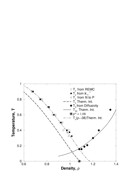
FIG. 2.: Liquid-gas spinodal obtained from (a) REMC simulations, (b) $k_{T}$, (c) polynomial fits to isotherms, and (d) the empirical free energy (‘$T_{s}$ Therm. Int.’). The same curve is also shown shifted in $\rho$ by 0.08 (‘$T_{s}(\rho-.08)$ Therm. Int.’). The glass transition locus obtained from (e) VFT fits to diffusivity data, and (d) extrapolation of configurational entropy to zero (‘$T_{IG}$ Therm. Int.’). Also marked (*) is the density $\rho^{*}$ where inherent structure pressure is a minimum.

An empirical free energy is constructed next, based on equilibrium data from MD simulations[6, 7, 11, 12, 13], which is used both to obtain an independent estimate of the spinodal, and to obtain a thermodynamic estimate of the glass transition locus. The absolute free energy $A(\rho,T)$ of the system at density $\rho$ at a reference temperature $T_{r}=3.0$ is first defined in terms of the ideal gas contribution $A_{id}(\rho,T)$ and the excess free energy $A_{ex}(\rho,T)$ obtained by integrating the pressure from simulations:

$$A(\rho,T)=A_{id}(\rho,T)+A_{ex}(\rho,T),$$ (1)

$$\beta A_{id}(\rho,T)=N\left(3~{}\ln\Lambda+\ln\rho-1\right),$$ (2)

$$\beta_{r}A_{ex}(\rho,T_{r})=\beta_{r}A^{0}_{ex}(0,T_{r})+N\int_{0}^{\rho}{d\rho^{{}^{\prime}}\over\rho^{{}^{\prime}}}\left({\beta_{r}P\over\rho^{{}^{\prime}}}-1\right),$$ (3)

$$\beta_{r}A^{0}_{ex}(0,T_{r})=-\ln{N!\over N_{A}!N_{B}!}.$$ (4)

Here, $N$ is the number of particles, $\beta\equiv k_{B}T$, $\Lambda$ is the de Broglie wavelength, and $A^{0}_{ex}$ arises from the mixing entropy. $A_{ex}$ is fit to a fifth order polynomial is $\rho$[14]. $A_{ex}$ at a desired temperature may be evaluated by integrating the potential energy, $E$:

$$\beta A_{ex}(\rho,\beta)=\beta A_{ex}(\rho,\beta_{r})+\int_{\beta_{r}}^{\beta}E(\rho,\beta^{{}^{\prime}})d\beta^{{}^{\prime}}$$ (5)

As observed in [6, 7], the $T$ dependence of $E$ at fixed, high, density is well described by the form $E(\rho,T)\sim T^{3/5}$, in agreement with predictions for dense liquids[15]. This form is not, however, accurate at low densities. In order to fit data well at low densities while retaining reliability at high densities, $E$ data for $\rho=0.55$ to $1.35$, and temperatures below $T=3.0$ are fitted to the form $E(\rho,T)/N=E_{0}(\rho)+E_{1}(\rho)T^{E_{2}(\rho)}$. The parameters $E_{0},E_{1},E_{2}$ are fitted polynomials in $\rho$[14]. These fits, which represent the measured MD data very well, together with the fit for $A^{0}_{ex}(0,T_{r}=3.0)$, define an empirical free energy from which the equation of state and the liquid-gas spinodal locus $\rho_{s}(T)$ are obtained via:

$$P(\rho,T)={\rho^{2}\over N}{\partial A(\rho,T)\over\partial\rho}~{}\vline_{{}_{{}_{{}_{~{}T}}}};~{}~{}~{}{\partial P\over\partial\rho}~{}\vline_{{}_{{}_{~{}\rho=\rho_{s}(T)}}}=0.$$ (6)

The liquid-gas spinodal locus resulting from the empirical free energy is shown in Fig. 2 and is seen to occur at lower densities than the REMC estimate, with a roughly constant shift in density (also shown in Fig. 2). Inspection of isotherms obtained from the empirical free energy (which show mean field behavior near the spinodal) reveals that while they agree very well with simulation isotherms away from the spinodal, they show deviations very close to the (REMC) spinodal densities. Correspondingly $k_{T}^{-1}$ obtained in simulations drops faster to zero close to the spinodal, while at higher densities there is very good agreement. The estimate from the empirical free energy must thus be considered a lower limit to the location of the spinodal.

Glass transition temperatures at the $7$ studied densities are obtained next, by fitting diffusion coefficients of $A$ particles to the Vogel-Fulcher-Tammann-Hesse (VFT) form:

$$D(\rho,T)=D_{o}(\rho)exp\left({A(\rho)\over T-T_{0}(\rho)}\right).$$ (7)

Values of $T_{0}(\rho)$ so estimated define lower limits to the laboratory glass transition $T_{g}$. The diffusion coefficients and the corresponding VFT fits are shown in Fig. 3. The resulting glass transition temperatures $T_{0}(\rho)$ are shown in Fig. 2. (Relaxation times yield very similar estimates. A qualitatively similar $T_{g}$ vs. $\rho$ curve has recently been reported in [16].)

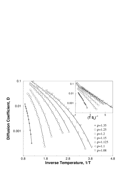
FIG. 3.: Arrhenius plot of diffusion coefficients and the corresponding VFT fits for the $7$ densities studied. (inset) Adam-Gibbs plot of diffusion coefficients against $(TS_{c})^{-1}$ and straight line fits.

A thermodynamic estimate of ideal glass transition temperatures is obtained next, by evaluating the configurational entropy of the liquid as a function of density and temperature. A number of studies in recent years[6, 7, 11, 12, 13, 17, 18, 19, 20, 21, 22] have focussed on evaluating of the configurational entropy[23]. The approach here, based on analyzing inherent structures[24], follows most closely those of Ref.s [6, 21, 7, 20]. The canonical partition function is re-written as a sum over all local potential energy minima, which introduces a distribution function for the number of minima at a given energy:

$$Q_{N}(\rho,T)=\Lambda^{-3N}{1\over N_{A}!N_{B}!}\int d{\bf r}^{N}exp\left(-\beta\Phi\right)$$ (8)

$$=\sum_{\alpha}exp\left(-\beta\Phi_{\alpha}\right)\Lambda^{-3N}\int_{V_{\alpha}}d{\bf r}^{N}exp\left(-\beta(\Phi-\Phi_{\alpha})\right)$$ (9)

$$=\int d\Phi_{\alpha}~{}\Omega(\Phi_{\alpha})~{}exp\left(-\beta(\Phi_{\alpha}+Nf_{basin}(\Phi_{\alpha},T))\right)$$ (10)

$$=\int d\Phi_{\alpha}~{}exp\left(-\beta(\Phi_{\alpha}+Nf_{basin}(\Phi_{\alpha},T)-TS_{c}(\Phi_{\alpha}))\right)$$ (11)

where $\Phi$ is the total potential energy of the system, $\alpha$ indexes individual inherent structures, $\Phi_{\alpha}$ is the potential energy at the minimum, $\Omega(\Phi_{\alpha})$ is the number density of inherent structures with energy $\Phi_{\alpha}$, and the configurational entropy $S_{c}\equiv k_{B}\ln\Omega$. The basin free energy $f_{basin}(\Phi_{\alpha},T)$ is obtained by a restricted partition function sum over a given inherent structure basin, $V_{\alpha}$. In the harmonic approximation, we have

$$\beta f={3\over 2}\ln({\beta\over 2\pi})+{1\over 2N}\sum_{i}^{3N-3}\ln\lambda_{i}\equiv\beta f_{therm}+\beta f_{vib},$$ (12)

where $\lambda_{i}$ are eigenvalues of the Hessian or curvature matrix at the minimum. $\beta f_{vib}$ is a slowly varying function of temperature (the temperature dependence is obtained by averaging over $1000$, $100$ inherent structures at $T<1.$, $T>1.$ respectively), and is fitted to the form $\beta f_{vib}(\rho,T)=f_{0}(\rho)+f_{1}(\rho)/T^{2}$ which fits available data quite well. Polynomial fits to $\rho$-dependent parameters $f_{0},f_{1}$ are obtained[14]. The total entropy of the liquid $S$ as well as the basin entropy $S_{basin}$ may be evaluated as a function of density and temperature from the total and basin free energies. The configurational entropy $S_{c}(\rho,T)$ and the ideal glass transition $T_{IG}(\rho)$ are then given by,

$$S_{c}(\rho,T)=S(\rho,T)-S_{basin}(\rho,T);S_{c}(\rho,T_{IG}(\rho))=0.$$ (13)

The ideal glass transition locus obtained is shown in Fig. 2, and is seen to be in very good agreement with the estimate based on diffusivity. Although such correlation is recorded for experimental data[25], it is noteworthy that $T_{0}$ estimates here from dynamic data at quite high $T$ produce such agreement. This agreement offers mutual support to the thermodynamic method followed here, and the feasibility of estimation based on dynamical measurements. $T_{IG}(\rho=1.2)=0.2976$ is in very good agreement with the values $0.297$ in [6] and $0.31$ in [7]. Diffusion coefficients plotted against $(TS_{c})^{-1}$ (inset of Fig. 3) show that the Adam-Gibbs expectation[23] $\ln{D}\sim(TS_{c})^{-1}$ is extremely well satisfied at all densities[12, 13, 25].

Data in Fig. 2 clearly indicate that the liquid-gas spinodal and glass transition loci would intersect at a finite temperature $T_{i}\sim 0.16$ (based on REMC data; $T_{i}\sim 0.12$ based on the empirical free energy). As this intersection happens at $\rho\sim\rho^{*}=1.08$, the data do not support the speculation that as $T\rightarrow 0$, $\rho_{s}(T)\rightarrow\rho^{*}$ or $\rho_{IG}(T)\rightarrow\rho^{*}$. On the other hand, $\rho^{*}$ does (within the uncertainty of the data) form the lower limiting density for glass formation. Experimental data (see e. g. [26]) for the P-dependence of $T_{g}$ indicate that $T_{g}(P)$ typically intersects the zero pressure axis, implying glass - gas coexistence and finite $T_{g}$ at negative pressures, a possibility implicit in [3] and also noted in [20]. However, intersection of the liquid-gas spinodal and the glass transition locus at a finite temperature observed here further implies an ideal glass - gas mechanical instability below $T_{i}$. Indirect evidence for this exists in the form of experimental $T_{g}(P)$ loci displaying a negative slope[26], but systematic evidence requires vitrification experiments at negative pressures[27].

A proper study of such a mechanical instability is beyond the scope of the present work, as it requires calculation of limits of stability accounting consistently for the presence of the three relevant phases (liquid, gas, glass). As a preliminary attempt, the equation of state of the glass below $T_{IG}(\rho)$ is obtained by noting that below $T_{IG}$ the system is trapped in the potential energy basin reached at $T_{IG}$. Details of such a calculation will not be presented here; Instead, two consequences are presented in Fig. 4. The inset demonstrates the slope discontinuity of the pressure at fixed density at $T_{IG}$ for $\rho=1.2$. The main diagram shows the isotherm at $T=0.05$ for the glass phase, which displays a mechanical instability density of $\rho\sim 1.$, where the slope vanishes, or, $k_{T}$ diverges.

FIG. 4.: Pressure vs. density for $T=0.05$ in the ideal glass phase (solid line), which exhibits a minimum at $\rho\sim 1.$. Extension of the liquid’s equation of state is shown for comparison (dashed line). Inset shows pressure vs. temperature across the ideal glass transition for $\rho=1.2$ (solid line).

An interesting by-product of the present analysis is the estimation of configurational entropy as a function of both energy and density, and a range of temperature dependences of dynamical quantities displaying a variable degree of fragility[28]. These data permit an evaluation of the relationship between fragility and configurational entropy[29], and will be presented elsewhere.

Useful discussions with and comments on the manuscript by C. A. Angell, D. S. Corti, C. Dasgupta, P. G. Debenedetti, F. Sciortino, R. J. Speedy and F. H. Stillinger are gratefully acknowledged.

REFERENCES

- [1] Email: sastry@jncasr.ac.in
- [2] Some recent reviews are articles in Science 267, (1995) and M. D. Ediger, C. A. Angell and S. R. Nagel, Supercooled Liquids and Glasses. J. Phys. Chem. 100, 13200 (1996).
- [3] S. Sastry, P. G. Debenedetti and F. H. Stillinger, Phys. Rev. E 56, 5533, (1997).
- [4] W. Kob and H. C. Andersen, Phys. Rev. E 51, 4626 (1995); K. Vollmayr, W. Kob and K. Binder J. Chem. Phys. 105, 4714 (1996).
- [5] S. Sastry, P. G. Debenedetti and F.H. Stillinger, Nature 393, 554 (1998).
- [6] F. Sciortino, W. Kob and P. Tartaglia, Phys. Rev. Lett. 83, 3214 (1997).
- [7] B. Coluzzi, G. Parisi and P. Verrocchio, J. Chem. Phys. 112 2933 (2000).
- [8] O. Penrose and J. L. Lebowitz, J. Stat. Phys. 3, 211 (1971).
- [9] D. S. Corti, Ph. D. thesis, Princeton University (1997);D. S. Corti and P. G. Debenedetti, Chem. Engg. Sci. 49, 2717 (1994).
- [10] As a binary mixture becomes unstable with respect to composition fluctuations prior to density fluctuations (see e. g. P. G. Debenedetti, Metastable Liquids (Princeton University Press, Princeton, 1996)) constraints were applied on the number of and particles separately.
- [11] R. J. Speedy, Mol. Phys. 80 1105 (1993); R. J. Speedy and P. G. Debenedetti, it Mol. Phys. 81 237 (1994);
- [12] R. J. Speedy, Mol. Phys. 95 169 (1998).
- [13] A. Scala, F. W. Starr, E. La Nave, F. Sciortino and H. E. Stanley, Nature (in press) (2000); cond-mat/9908301.
- [14] The fit parameters for various quantities are: , , , and , , .
- [15] Y. Rosenfeld and P. Tarazona, Mol. Phys. 95, 141 (1998).
- [16] R. Di Leonardo, L. Angelani, G. Pariso and G. Ruocco, (preprint) cond-mat/0001311.
- [17] L. Angelani, G. Parisi, G. Ruocco and G. Viliani, Phys. Rev. Lett. 81 4648 (1998).
- [18] M. Cardenas, S. Franz and G. Parisi, J. Phys. A: Math. Gen. 31, L163 (1998).
- [19] M. Mezard and G. Parisi, Phys. Rev. Lett. 82, 747 (1999); M. Mezard, Physica A 265, 352 (1999); M. Mezard and G. Parisi, J. Chem. Phys. 111, 1076 (1999).
- [20] B. Coluzzi, M. Mezard, G. Parisi and P. Verrocchio, J. Chem. Phys. 111, 9039 (1999); B. Coluzzi, G. Parisi and P. Verrocchio, Phys. Rev. Lett. 84, 306 (2000).
- [21] S. Buechner and A. Heuer, Phys. Rev. E 60, 6507 (1999); Phys. Rev. Lett. 84, 2168 (2000).
- [22] P. G. Debenedetti, F. H. Stillinger, T. M. Truskett and C. J. Roberts, J. Phys. Chem. B 103, 7390 (1999).
- [23] J.H. Gibbs and E. A. Di Marzio J. Chem. Phys. 28, 373 (1958); G. Adams and J.H. Gibbs J. Chem. Phys. 43, 139 (1958).
- [24] F.H. Stillinger and T.A. Weber, Phys. Rev. A 25, 978 (1982); Science 225, 983 (1984); F.H. Stillinger, Science 267, 1935 (1995).
- [25] C. A. Angell, J. Res. Natl. Stand. Technol. 102 171 (1997).
- [26] E. Williams and C. A. Angell, J. Phys. Chem. 81, 232 (1977).
- [27] C. A. Angell and Zheng Qing, Phys. Rev. B, Rapid Comm., 39, 8784,(1989).
- [28] C. A. Angell, J. Non-Cryst. Solids 131-133, 13 (1991).
- [29] R. J. Speedy, J. Phys. Chem. B 103, 4060 (1999).