Optical conductivity of one-dimensional Mott insulators

Abstract

We calculate the optical conductivity of one-dimensional Mott insulators at low energies using a field theory description. The square root singularity at the optical gap, characteristic of band insulators, is generally absent and appears only at the Luther-Emery point. We also show that only few particle processes contribute significantly to the optical conductivity over a wide range of frequencies and that the bare perturbative regime is recovered only at very large energies. We discuss possible applications of our results to quasi one-dimensional organic conductors.

Measurements of dynamical properties and in particular the optical conductivity $\sigma(\omega)$ are supposed to provide a stringent test of the existing theories of quasi one-dimensional (1D) systems. The behaviour of $\sigma(\omega)$ in the metallic regime is easily understood in terms of the Tomonaga-Luttinger theory [1]. The situation in the Mott insulating phase [2] is much more complicated as a spectral gap is dynamically generated by interactions. Here $\sigma(\omega)$ has until now only been studied by perturbative methods [4, 5], which are expected to work well at high and intermediate frequencies but are not applicable to the most interesting regime of frequencies close to the optical gap. The purpose of the present work is to determine $\sigma(\omega)$ in 1D Mott insulators for all frequencies much smaller than the bandwidth, which is the large scale in the field theory approach to the problem. In particular we obtain for the first time the true behaviour of $\sigma(\omega)$ just above the optical gap.

An important property of one-dimensional systems that significantly simplifies our analysis is spin-charge separation, which occurs at energies much smaller than the bandwidth. In this regime $\sigma(\omega)$ is determined solely by the charge degrees of freedom. The standard description of the charge sector of 1D Mott insulator is given by the sine-Gordon model (SGM) [3, 5]

$$H_{sG}=\int\mbox{d}x\left[4\pi(\Pi)^{2}+\frac{1}{16\pi}(\partial_{x}\phi)^{2}+2\mu\cos(\beta\phi)\right].$$ (1)

Here the momentum and coordinate densities obey the standard commutation relation $[\Pi(x),\phi(y)]=-i\delta(x-y)$. Throughout this letter we set the charge velocity and $\hbar$ equal to one.

The cosine term in the Hamiltonian is related to Umklapp processes and the value of the sine-Gordon coupling constant $\beta$ is determined by the interactions. The Umklapp processes are relevant for $\beta^{2}<1$ and dynamically generate a spectral gap $M$, which is related to $\mu$ by (30). For $1/2<\beta^{2}<1$ the spectral gap is related to optical gap $\Delta$ (i.e. the gap seen in the optical absorption) by $\Delta=2M$ whereas for $\beta^{2}<1/2$ solitonic bound states are formed below $2M$.

Our calculations of $\sigma(\omega)$ are based on the exact solution of the SGM and in particular on the work of Smirnov [6]. We confine our analysis to the repulsive regime $1/2<\beta^{2}<1$, where the excitation spectrum consists of charged particles and holes (solitons and anti-solitons), which do not form bound states. At the “Luther-Emery” point $\beta^{2}=1/2$ the SGM is equivalent to the theory of free spinless massive Dirac fermions. In this limit the solitons become non-interacting particles and the Mott insulator turns into a conventional band insulator. In the limit $\beta^{2}\rightarrow 1$ the SGM acquires an SU(2) symmetry and describes the Hubbard model at half-filling in the regime of weak interactions [7, 8] and $\sigma(\omega)$ was recently determined in [9].

The optical conductivity is related to the imaginary part of the current-current correlation function, $\chi(\omega,q)=\langle j_{-q}\;j_{q}\rangle$ by

$$\sigma(\omega>0)={\rm Im}\left\{\chi(\omega,q=0)\right\}/\omega.$$ (2)

The current density operator is proportional to the momentum density

$$j_{q}=A^{1/2}\Pi_{q},~{}~{}\Pi_{q}=\int dx\Pi(t,x)e^{iqx}\ .$$ (3)

The non-universal coefficient $A^{1/2}$ depends on the detailed structure of the underlying microscopic lattice model.

Using the spectral representation one can express the optical conductivity at $T=0$ as a sum over matrix elements of the zero wave vector Fourier component of the momentum operator:

$$\sigma(\omega>0)=\frac{A}{\omega}\sum_{n}|\langle 0|\Pi_{0}|n\rangle|^{2}\delta[\omega-(E_{n}-E_{0})].$$ (4)

Here $|0\rangle$ and $|n\rangle$ represent the ground state and excited states with energies $E_{0}$ and $E_{n}$ respectively. The difficulties in computation of the optical response are related to the fact that one requires not only the knowledge of the spectrum $E_{n}$, but also of the matrix elements of the momentum operator. The exact expressions for the matrix elements $\langle n|\Pi_{0}|0\rangle$ are extracted from the exact solution by means of the so-called form factor bootstrap procedure [6]. This approach is particularly efficient for strongly interacting integrable models with spectral gaps, because for a given energy $\omega$ the spectral representation for the imaginary part contains only a finite number of terms (in the absence of bound states at most $[\omega/\Delta]$ terms). In practice the spectral sum is found to converge extremely rapidly, so that a very good approximate description can be obtained by taking into account intermediate states with at most four particles [10]. The multi-particle matrix elements become essential only at very high energies where the field theory can no longer be used to describe the underlying lattice model anyway.

In order to compute (4) we need to introduce a suitable spectral representation. In the parameter regime we study, the spectrum contains only solitons and anti-solitons with relativistic dispersion $e(p)=\sqrt{p^{2}+M^{2}}$. It is useful to parametrize the spectrum in terms of a rapidity variable $\theta$

$$p=M\sinh\theta,\>e=M\cosh\theta\ ,\qquad$$ (5)

Solitons and anti-solitons are distinguished by the internal index $\varepsilon=\pm$. A state of $n$ solitons/anti-solitons with rapidities $\{\theta_{k}\}$ and internal indices $\{\varepsilon_{k}\}$ is denoted by: $|\theta_{n}\ldots\theta_{1}\rangle_{\varepsilon_{n}\ldots\varepsilon_{1}}$. Its total energy $E$, momentum $P$ and electric charge $Q$ are:

$$P=M\sum_{k=1}^{n}\sinh\theta_{k},\ E=M\sum_{k=1,}^{n}\cosh\theta_{k},\ Q\propto\sum_{k=1}^{n}\varepsilon_{k}\ .$$ (6)

In terms of this basis $\sigma(\omega)$ is expressed as

$$\sigma(\omega) = \frac{2\pi^{2}A}{\omega}\sum_{n=0}^{\infty}\sum_{\varepsilon_{i}}\int\frac{\mbox{d}\theta_{1}\ldots\mbox{d}\theta_{n}}{(2\pi)^{n}n!}\left|f^{j}(\theta_{1}\ldots\theta_{n})_{\varepsilon_{1}\ldots\varepsilon_{n}}\right|^{2}$$ (7)

$$\times \delta(M\sum_{k}\sinh\theta_{k})\delta(\omega-M\sum_{k}\cosh\theta_{k})$$ (8)

$$= \sigma_{2}(\omega)+\sigma_{4}(\omega)+...$$ (9)

Here

$$f^{j}(\theta_{1}\ldots\theta_{n})_{\varepsilon_{1}\ldots\varepsilon_{n}}\equiv\langle 0|j(0,0)|\theta_{n}\ldots\theta_{1}\rangle_{\varepsilon_{n}\ldots\varepsilon_{1}}$$ (10)

are the form factors of the current operator, $\sigma_{2}(\omega)$ and $\sigma_{4}(\omega)$ represent the contributions from 2 and 4-particle processes and the dots indicate processes involving higher number of (anti)solitons. We note that as a consequence of symmetry properties only intermediate states with an even number of particles contribute to this correlation function. From (9) it is easy to see that only 2-particle processes contribute up to energies $\omega=4M$, only 2 and 4-particle processes up to $\omega=6M$ and so on.

The form factors (10) have been determined in [6] and can be used to calculate the first few terms in the expansion (9). We find

$$\sigma_{2}(\omega)=\frac{2A\Theta(\omega-2M)}{{\omega^{2}}\sqrt{{\omega}^{2}-4M^{2}}}|f(\theta)|^{2}\ ,$$ (11)

where $\Theta(x)$ is the Heaviside function,

$$f(\theta)=f^{j}(\theta)_{+-}=f^{j}(\theta)_{-+}=\frac{2\pi M}{i\beta}\frac{\sinh{\theta/2}}{\cosh{\left(\frac{\theta+i\pi}{2\xi}\right)}}$$ (12)

$$\times\exp\left\{\int_{0}^{\infty}dt\;\frac{\sinh^{2}{t(1-i\theta/\pi)}\sinh{t(\xi-1)}}{t\sinh{2t}\cosh{t}\sinh{t\xi}}\right\}$$ (13)

and

$$\theta=2{\rm arccosh(\tilde{\omega})}\ ,\ \xi=\beta^{2}/(1-\beta^{2})\ ,\ \tilde{\omega}=\omega/2M.$$ (14)

The four particle contribution is of the form

$$\sigma_{4}(\omega)=\frac{\Theta(\omega-4M)}{192\omega\pi^{2}M^{2}}\sum_{\varepsilon_{i}}\sum_{\sigma=\pm}\int_{-a}^{a}d\theta\;\int_{-b(\theta)}^{b(\theta)}d\gamma$$ (15)

$$\times|f^{j}(g-\frac{\sigma\alpha}{2},g+\frac{\sigma\alpha}{2}g+\theta+\gamma,g-\theta+\gamma)_{\varepsilon_{1}...\varepsilon_{4}}|^{2}$$ (16)

$$\times\left\{\left(\sqrt{\cosh^{2}{\theta}\sinh^{2}{\gamma}+\tilde{\omega}^{2}}-\cosh{\theta}\cosh{\gamma}\right)^{2}-1\right\}^{-\frac{1}{2}}$$ (17)

$$\times\left[\cosh^{2}{\theta}\sinh^{2}{\gamma}+\tilde{\omega}^{2}\right]^{-\frac{1}{2}}\ ,$$ (18)

where

$$a = {\rm arccosh(\tilde{\omega}-1)},\ b(\theta)={\rm arccosh\left[\frac{\tilde{\omega}^{2}-1-\cosh^{2}{\theta}}{2\cosh{\theta}}\right]},$$ (19)

$$g = \ln\left[\frac{\cosh(\alpha/2)+\exp(-\gamma)\cosh\theta}{\tilde{\omega}}\right],$$ (20)

$$\alpha = 2{\rm arccosh}\left[\sqrt{\cosh^{2}{\theta}\sinh^{2}{\gamma}+\tilde{\omega}^{2}}-\cosh{\theta}\cosh{\gamma}\right].$$ (21)

The four particle form factor is given by

$$f^{j}(\beta_{1},...,\beta_{4})_{--++}=\frac{4\pi^{3}}{\beta}\xi Md^{2}\prod_{k<l}\zeta(\beta_{k}-\beta_{l})$$ (22)

$$\times \prod_{m,n=1,2}\left({\sinh[(\beta_{2+m}-\beta_{n}-i\pi)/\xi]}\right)^{-1}$$ (23)

$$\times 2\sinh[{(\beta_{4}+\beta_{3}-\beta_{1}-\beta_{2}-2\pi i)/2\xi}]$$ (24)

$$\times \exp(-\frac{1}{\xi}\sum_{k}\beta_{k})\int\frac{\mbox{d}\alpha}{i\pi}\prod_{k}\varphi(\alpha-\beta_{k})\cosh(\alpha-\frac{1}{2}\sum_{k}\beta_{k})$$ (25)

$$\times \Delta(e^{2\alpha/\xi}|e^{2\beta_{1}/\xi},e^{2\beta_{2}/\xi}|e^{2\beta_{3}/\xi},e^{2\beta_{4}/\xi}).$$ (26)

The different orderings for (22) that appear in (15) can be obtained using the following property of the form factors

$$f^{j}(\theta_{1}\ldots\theta_{i}\theta_{i+1}\ldots\theta_{n})_{\varepsilon_{1}\ldots\varepsilon_{i}\varepsilon_{i+1}\ldots\varepsilon_{n}}S^{\varepsilon_{i}\varepsilon_{i+1}}_{\varepsilon_{i}^{\prime}\varepsilon_{i+1}^{\prime}}(\theta_{i}-\theta_{i+1})$$ (27)

$$=f^{j}(\theta_{1}\ldots\theta_{i+1}\theta_{i}\ldots\theta_{n})_{\varepsilon_{1}\ldots\varepsilon_{i+1}^{\prime}\varepsilon_{i}^{\prime}\ldots\varepsilon_{n}}\ ,$$ (28)

where $S$ is the two body scattering matrix. The various functions appearing in Eqs (22) and (28) can be found in [6] (note that our definition of $\xi$ differs by a factor of $\pi$).

FIG. 1.: Two particle (solind line) and one hundred times the four-particle (dashed line) contributions to the optical conductivity as a function of $(\omega/M)$ for $\beta^{2}=0.9$. Inset: threshold behaviour of the optical conductivity close to the Luther-Emergy point for four different values of $\beta$; $\beta=0.75$ (solid), $\beta=0.74$ (dotted), $\beta=0.73$ (dashed) and $\beta=0.72$ (long dashed) .

The two and (one hundred times the) four-particle contributions to $\sigma(\omega)$ for $\beta^{2}=0.9$ are presented in Fig.1. Most importantly, the square root singularity, being a characteristic feature of band insulators, is suppressed by the momentum dependence of the soliton-antisoliton form factor and reappears only for the Luther-Emery point $\beta^{2}=1/2$. This effect was noted previously for the Hubbard model at half-filling [9] which corresponds to the special SU(2)-symmetric point $\beta^{2}=1$. We find that for any $\beta^{2}\neq 1/2$ there is a square root “shoulder” $\sigma(\omega)\propto\sqrt{\omega-\Delta}$ for $\omega/\Delta-1\ll 1$ as is shown in the inset of Fig.1. In the vicinity of the Luther-Emery point $\beta^{2}=1/2$ we obtain the following analytical expression valid for ${\tilde{\omega}}-1\ll 1$:

$$\sigma(\omega)\propto\frac{\sqrt{\tilde{\omega}^{2}-1}}{[\tilde{\omega}^{2}-1]+\xi^{2}\sin^{2}\gamma},~{}~{}\gamma=\pi\left(\frac{1}{2\beta^{2}}-1\right).$$ (29)

The square root singularity above $\omega=\Delta$ for $\beta^{2}=1/2$ is replaced by a maximum occurring at $\omega/\Delta-1\propto\gamma^{2}$.

The four particle contribution to $\sigma$ is seen to be insignificant at low energies and becomes larger than the two particle contribution only at $\omega\approx 180M$ for $\beta^{2}=0.9$. This suggests that the optical conductivity is well described by the combination of 2 and 4-particle contributions up to several hundred times the mass gap. Computation of higher order terms in Eq.(9) becomes cumbersome and probably of no physical interest, since the previous analysis suggests that they become important outside the region of applicability of the field theory approach to physical systems.

At frequencies much larger than the gap it is possible to determine $\sigma(\omega)$ by perturbative methods. The leading asymptotics can be calculated by “conformal perturbation theory” [11]. Here the cosine interaction in (1) is considered as a (relevant) perturbation of the Gaussian model and correlation functions are calculated in a perturbative expansion in powers of the scale $\mu$, which then can be expressed in terms of the physical gap $M$ as [12]

$$\mu=\frac{\Gamma(\beta^{2})}{\pi\Gamma(1-\beta^{2})}\left[M\frac{\sqrt{\pi}\Gamma(1/2+\xi/2)}{2\Gamma(\xi/2)}\right]^{2-2\beta^{2}}.$$ (30)

We find to leading order

$$\sigma(\omega)=2^{9-4\beta^{2}}\left(\frac{\pi^{2}\beta}{\Gamma(2\beta^{2})}\right)^{2}\mu^{2}\omega^{(4\beta^{2}-5)}$$ (31)

$$=\frac{8\pi^{3}\beta^{2}}{\omega\Gamma^{2}(1-\beta^{2})\Gamma^{2}(\frac{1}{2}+\beta^{2})}\left[\frac{\Gamma(\frac{\xi}{2})}{2\sqrt{\pi}\Gamma(\frac{1+\xi}{2})}\frac{\omega}{M}\right]^{4\beta^{2}-4}.$$ (32)

We emphasize that the ratio of the coefficients of the high- and low-energy asymptotics (32), (11) is fixed [6],[13]. In other words, the amplitude of the power law in (32) is tied to the overall factor in (11) and the form factor expansion must approach the perturbative result in the large-$\omega$ limit. A comparison between the form factor results and (32) is shown in Fig.2. We see that the asymptotic regime is not yet reached at energies as high as $\omega\sim 1000M$ (in practical terms this implies that perturbation theory cannot be used to make contact with experiment). We note that the contributions due to intermediate states with 6,8,10 … particles are all positive and will make the agreement of the form factor sum with perturbation theory in the region $\omega\approx 1000M$ only worse. A good way to overcome these deficiencies of bare perturbation theory is to carry out a renormalisation-group (RG) improvement as performed in [4]. In Zamolodchikov’s scheme [12] the RG equations for the Sine-Gordon model are given by

$$\frac{dg_{\perp}}{dt}=\frac{g_{\parallel}g_{\perp}}{1+\frac{g_{\parallel}}{2}}\ ,\quad\frac{dg_{\parallel}}{dt}=\frac{g^{2}_{\perp}}{1+\frac{g_{\parallel}}{2}}\ .$$ (33)

The solution of (33) is

$$g_{\perp}=4\frac{1-\beta^{2}}{\beta^{2}}\frac{\sqrt{q}}{1-q}\ ,\quad g_{\parallel}=2\frac{1-\beta^{2}}{\beta^{2}}\frac{1+q}{1-q}\ ,$$ (34)

where

$$q\left(\frac{(1-q)\beta^{2}}{4(1-\beta^{2})}\right)^{2\beta^{2}-2}=e^{(4-4\beta^{2})(t-t_{0})}.$$ (35)

Using $t-t_{0}=\ln\left(\frac{\sqrt{\pi}e^{3/4}M}{2^{3/2}\omega}\right)$ we can reexpress (32) up to higher order terms as

$$\sigma(\omega)=\frac{\pi^{3}\beta^{6}g_{\perp}^{2}}{2\omega\Gamma^{2}(2-\beta^{2})\Gamma^{2}(\frac{1}{2}+\beta^{2})}\left[\frac{\Gamma(\frac{\xi}{2})e^{3/4}\sqrt{\xi}}{2^{7/2}\Gamma(\frac{1+\xi}{2})}\right]^{4\beta^{2}-4}.$$ (36)

The RG improved result (36) for $\sigma(\omega)$ is compared to the form factor result (sum of the two and four-particle contributions) in the inset of Fig.2. The agreement is rather good down to energies of the order of $5M$.

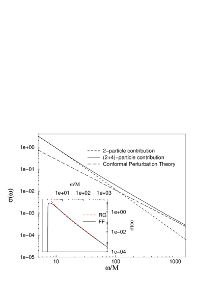
FIG. 2.: Comparison between the 2 and 2+4-particle contribution to the optical conductivity and the perturbative result, for $\beta^{2}=0.9$. Inset: comparison between the form factor result and RG improved perturbation theory.

One possible realisation of a 1D Mott insulator are the $\rm(TMTSF)_{2}X$ Bechgaard salts [14]. These materials are highly anisotropic and can be modelled as weakly coupled, quarter-filled chains. At energies or temperatures above the 1D-3D crossover scale $E_{\rm cr}$ the interchain coupling becomes ineffective and a description in terms of a purely 1D model with charge sector (1) should be possible [5]. At present there is some uncertainty regarding the value of $E_{\rm cr}$ because interactions can renormalize its bare value, set by the interchain coupling, downwards [15]. There is a lot of ambiguity in fitting our results to the data. The value of the optical gap $2M$ is not known and, as discussed above, we cannot calculate the overall normalisation of $\sigma(\omega)$. We therefore use these as parameters in order to obtain a good fit at large $\omega$ (where the theory is expected to work best as 3D effects are unimportant) to the data [14] for any given value of $\beta$. We obtain reasonable agreement with the data for $\beta^{2}\approx 0.9$, which corresponds to a Luttinger liquid parameter of $K_{\rho}\approx 0.23$. This value is consistent with previous estimates (see the discussion in [14]).

FIG. 3.: Comparison between the optical conductivity calculated in the SGM for $\beta^{2}=0.9$ (solid lines) and measured optical conductivity for $\rm(TMTSF)_{2}PF_{6}$ from Ref.[12] (diamonds). The inset shows the same comparison on a logarithmic scale.

As is clear from Fig. 3, the model (1) seems to apply well at high energies, but becomes inadequate at energies of the order of about $10$ times the Mott gap ($\approx 1600/{\rm cm}$ in $\rm(TMTSF)_{2}PF_{6}$). Spectral weight is transferred to lower energies and physics beyond that of a pure 1D Mott insulator emerges. There are at least two mechanisms that should be taken into account in this range of energies. Firstly, a small dimerization occurs in the 1D chains and will almost certainly affect the structure of $\sigma(\omega)$ around its maximum. Secondly, the interchain hopping is no longer negligible [16] and ought to be taken into account.

In summary, we have exactly calculated $\sigma(\omega)$ for a pure 1D Mott insulator in a low-energy effective field theory approach. We have determined the threshold behaviour for the first time and found it to exhibit a universal square root increase for any $\beta^{2}>1/2$. This is in contrast to the well-known suqare-root singularity that appears at the Luther-Emery point $\beta^{2}=1/2$. In the “low” energy region ($\omega/\Delta<50$) the optical conductivity is dominated by the two-particle form factor contribution with a small correction from four-particle processes. This means that the entire optical transport is dominated by two-particle processes! We furthermore have shown that the leading asymptotic behaviour obtained in perturbation theory is a good approximation only at extremely large frequencies, whereas RG-improved perturbation theory works well over a large region of energies.

We are grateful to A. Schwartz for generously providing us with the experimantal data and to F. Gebhard, T. Giamarchi, E. Jeckelmann and S. Lukyanov for important comments and discussions. We thank the Isaac Newton Institute for Mathematical Sciences, where this work was completed, for hospitality.

REFERENCES

-
[1]
See e.g. Bosonization in Strongly Correlated
Systems A. O. Gogolin, A. A. Nersesyan and A. M. Tsvelik,
Cambridge University Press (1999),
J. Voit, Rep. Progr. Phys. 58, 977 (1995). - [2] N. F. Mott, Metal-Insulator Transitions, ed., Taylor and Francis, London (1990); F. Gebhard, The Mott Metal-Insulator Transition, Spinger, Berlin (1997).
- [3] V.J. Emery, A. Luther and I. Peschel, Phys. Rev. B13, 1272 (1976).
- [4] T. Giamarchi Phys. Rev. B44 (1991) 2905.
- [5] T. Giamarchi Phys. Rev. B46, 342 (1992); Physica B 230-232, 975 (1997).
-
[6]
F. A. Smirnov, Form Factors in Completely Integrable Models of
Quantum Field Theory, World Scientific,
Singapore (1992). - [7] I. Affleck, talk given at the Nato ASI on Physics, Geometry and Topology, Banff, August 1989.
- [8] F. H. L. Essler and V. E. Korepin, Phys. Rev. Lett. 72, 908 (1994); Nucl. Phys. B426, 505 (1994).
- [9] E. Jeckelmann, F. Gebhard and F.H.L. Essler, preprint cond-mat/9911281.
- [10] J. Cardy and G. Mussardo Nucl. Phys. B410 (1993) 451; F. Lesage, H. Saleur and S. Skorik Nucl. Phys. B474 (1996) 602; J. Balog and M. Niedermaier, Nucl. Phys. B500 (1997) 421.
- [11] Al. B. Zamolodchikov, Nucl. Phys. B348, 619 (1991); V. A. Fateev, D. Fradkin, S. Lukyanov, A. B. Zamolodchikov and Al. B. Zamolodchikov Nucl. Phys. B540 (1999) 587.
- [12] Al. B. Zamolodchikov, Int. J. Mod. Phys. A 10, 1125 (1995).
- [13] S. Lukyanov, Mod. Phys. Lett.A12, 2543 (1997).
- [14] A. Schwartz, M. Dressel, G. Grüner, V. Vescoli, L. Degiorgi, T. Giamarchi Phys. Rev. B58 (1998) 1261 and references therein; V. Vescoli, L. Degiorgi, W. Henderson, G. Grüner, K. P. Starkey, L. K. Momtgomery, Science 281, 1181 (1998).
- [15] D. Boies, C. Bourbonnais and A.-M.S. Tremblay, Phys. Rev. Lett. 74,968 (1995).
- [16] A. Georges, T. Giamarchi and N. Sandler, preprint cond-mat/0001063 .