Theoretical Results for Sandpile Models of SOC with Multiple Topplings

Abstract

We study a directed stochastic sandpile model of Self-Organized Criticality, which exhibits recurrent, multiple topplings, putting it in a separate universality class from the exactly solved model of Dhar and Ramaswamy. We show that in the steady-state all stable states are equally likely. Then we explicitly derive a discrete dynamical equation for avalanches on the lattice. By coarse-graining we arrive at a continuous Langevin equation for the propagation of avalanches and calculate all the critical exponents characterizing them. The avalanche equation is similar to the Edwards-Wilkinson equation, but with a noise amplitude that is a threshold function of the local avalanche activity, or interface height, leading to a stable absorbing state when the avalanche dies. It represents a new type of absorbing state phase transition.

PACS numbers: 05.65.+b, 87.23.Ge, 87.23.Kg

I Introduction

Sandpile models of stick-slip dynamics have received considerable attention as canonical models of self-organized criticality (SOC) [1]. SOC refers to the widespread tendency of many extended, dissipative dynamical systems to evolve inevitably towards a complex state with power-law correlations in space and time: a “critical” state. Of course, a critical state is only one possible example of complex phenomena that can emerge in large, self-organizing systems composed of many strongly interacting parts. No doubt there are other types of complex states that have not yet been so well characterized mathematically, e.g. for example in networks [2]. From this viewpoint, the phenomena of SOC itself is a prototype for how complexity emerges in nature without fine tuning parameters. In spite of the gross simplicity of various cellular models that have been introduced, and hundreds if not thousands of numerical studies of SOC, only minimal analytic understanding has been achieved.

In fact, a survey of analytic works on sandpile models of SOC is exceedingly short. The model of SOC introduced by Bak, Tang, and Weisenfeld (BTW) [3] has yielded to some analytic treatment associated with its abelian properties, primarily due to the work of Dhar and collaborators [4]. The scaling properties of waves, where each site only topples, or releases grains, once has been understood by Priezzhev and collaborators [5, 6]. Nevertheless, the large scale properties of avalanches, where each site can topple many times in response to a single grain being added to the system, remain unsolved and the numerical situation controversial [6, 7, 8, 9]. The same is true for the Zhang model where some limited progress has been made using methods from dynamical systems theory [10]. Recurrent, multiple topplings within an avalanche also appear in most other unsolved sandpile models, such as the stochastic Manna model [11], the universality class [13] represented by the Oslo rice pile model [12], cellular models of vortex dynamics [14], as well as one-dimensional trough models exhibiting multiscaling [15]. The difficulties preventing progress in solving any of these simplified models in particular, or finding general analytic tools for granular systems exhibiting SOC, appear to be related, in part, to the existence of recurrent topplings.

This statement is further supported by the following facts: Dhar and Ramaswamy (DR) [16] introduced a directed version of the BTW model, and solved for the avalanche distribution and many other properties exactly. In the DR model, it can be rigorously proven that no multiple topplings occur. (Consequently, the elegant DR solution, as it has been conceived thus far, does not address the full complexity of discrete or granular models of SOC.) The fixed scale transformation method of Pietronero and collaborators [17] also explicitly ignores the presence of multiple topplings. One consequence of this fact is that this method puts the stochastic Manna model and the BTW model into the same universality class, which is not consistent with most numerical works [7, 18] (except [8]), including those measuring unequivocal differences in aging behaviors [19]. Multiple topplings, where the activity can return an arbitrarily large number of times, do not appear in any mean field description [20], since in high enough dimensions, the avalanche activity is not recurrent, or able to return more than a finite number of times [21], at any site. Multiple topplings are a fluctuation effect associated with self-intersections of the avalanche cluster in space and time [22], and as such are relevant below some upper critical dimension.

Certainly, the intricacies associated with multiple topplings are not the only ones that present themselves in attempting an analytic treatment of granular models of SOC. For example, the fact that the dissipation process is confined to the boundary, which forces the system to self-organize, is an important and subtle point because the boundary cannot be scaled out in the limit of large system sizes as is usually done in statistical physics. In principle, the boundary is always important, because the incoming sand grains must be transported to it, no matter how large the system size. The broken translational invariance associated with the boundary often leads to long range boundary effects in the metastable states (see, for example, [23, 24]). It might be useful to pry these complications apart, treating one issue at a time. Here we focus on the problem of recurrent or multiple topplings, and seek a model which does not present other difficulties.

Recently, Pastor-Satorras and Vespignani [25] have studied numerically a stochastic directed sandpile model (SDM), which is a stochastic version of the exactly solvable model introduced by DR. This stochastic model is simpler and presumably unrelated to the directed models introduced and studied by Tadić and collaborators [26]. Pastor-Satorras and Vespignani demonstrated by numerical simulations that the model exhibits multiple topplings which changes the universality class, making it distinct from the DR model. This was accomplished by numerically measuring and comparing various critical exponents characterizing the avalanches. Its close relation to the DR model, which has an exact solution, suggests to us an analytic study.

A Summary

We proceed with an analysis of the SDM as follows: First we define the DR model and the SDM. For pedagogical reasons, in Section III, we review the proof that the critical state of the DR model is the set of all stable states with equal probability. We also review some necessary parts of Dhar’s construction of an operator algebra for stochastic models, which can be represented as deterministic models with a quenched array of random numbers. Combining these two works, we then show that for the SDM the critical state is also the set of all stable states with equal probability, described by a product measure. Using this fact, we show in Section IV that the SDM can be recast as a generalized branching process propagating in an uncorrelated environment, enabling a study of the infinite system. By carefully analyzing the microscopic dynamics of this process on the lattice, we explicitly derive a discrete dynamical equation for the propagation of flowing grains in avalanches. In Section V, coarse graining this discrete equation gives a continuum equation for avalanches that should describe the large scale properties of any microscopic model with the same symmetry, conservation of grains, and stochastic effects.

Notably, our equation is similar to the Edwards-Wilkinson (EW) equation [27] except that the amplitude of the nonconservative noise is a Heaviside (theta) function of the local activity. Crucially, the noise amplitude is a threshold function, rather than being a constant, such as the temperature. The height of the interface represents the number of topplings in an avalanche. The steady state that is eventually reached in the limit of large times is always the state of no activity where the height of the interface is zero everywhere and the avalanche has died. Thus the equation describing avalanche dynamics corresponds to an absorbing state phase transition where the the transient state is governed by the EW equation in the region where it survives. Section V also describes an analysis of this nonlinear equation. We extract all the (nontrivial) critical exponents for avalanches, i.e. in $d=1$, $D=7/4$, $\tau=10/7$, $z=2$, $\tau_{t}=D=7/4$ distinct from the DR model. For $d\geq 2$, where multiple topplings are not relevant, the critical exponents are the same as in the DR model. All of these results agree perfectly with previous numerical works [25, 28]. We also write down the Fokker-Planck equation for the probability distribution of the number of topplings at each site in an avalanche, although we do not solve it. Finally, we conclude with a brief comment on some possibilities for future analytical work on absorbing state phase transitions and granular models of SOC.

II Definition of Directed Models

Consider a two dimensional square lattice as shown in Fig.  1. The direction of propagation is labeled by $t$, with $0\leq t<T$. The transverse direction is labeled by $x$, with periodic boundary conditions. Only sites with $(x+t)$ even are on the lattice, so that $x$ is a positive integer modulo $2X$, and the lattice has a total of $TX$ sites. On each site, an integer variable $z(x,t)$ is assigned. The $i$’th grain is added to a randomly chosen site $x_{i}$ on the top row $t=0$. There $z(x_{i},0)\rightarrow z(x_{i},0)+1$. When any site acquires a height greater than $z_{c}=1$ it topples, i.e. $z(x,t)\rightarrow z(x,t)-2$ for $z(x,t)>z_{c}$.

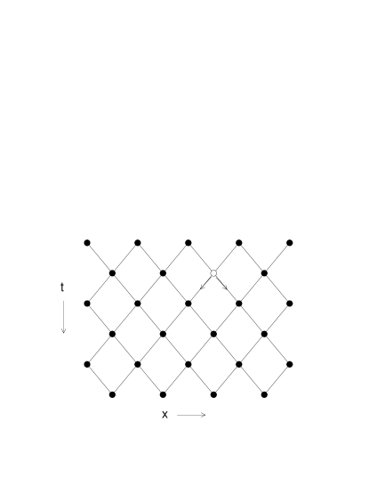
FIG. 1.: Directed Sandpile Models Grains from active sites in row $t$ topple onto sites in row $t+1$. For example, grains from the site indicated by the open circle topple only onto the nearest neighbor sites indicated by the arrows.

The two models differ with respect to the transmission of grains out of a toppling site. In the DR model, one grain is transferred to the left downstream neighbor and one grain to the right so the toppling rule is for $z(x,t)>z_{c}$

$$z(x,t) \rightarrow z(x,t)-2$$ (1)

$$z(x-1,t+1) \rightarrow z(x-1,t+1)+1$$ (2)

$$z(x+1,t+1) \rightarrow z(x+1,t+1)+1\,\,.$$ (3)

For the SDM, on the other hand, each grain from a toppling site is given equal probability to go to any downstream nearest neighbor. In this case, when the site $(x,t)$ topples,

$$z(x,t)\rightarrow z(x,t)-2$$

and

$$z(x-1,t+1) \rightarrow z(x-1,t+1)+1$$ (4)

$$z(x+1,t+1) \rightarrow z(x+1,t+1)+1\,\,$$ (5)

with probability 1/2, or

$$z(x-1,t+1) \rightarrow z(x-1,t+1)+2$$ (6)

$$z(x+1,t+1) \rightarrow z(x+1,t+1)\,\,$$ (7)

with probability 1/4, or

$$z(x-1,t+1) \rightarrow z(x-1,t+1)$$ (8)

$$z(x+1,t+1) \rightarrow z(x+1,t+1)+2\,\,.$$ (9)

with probability 1/4. Thus, the SDM is a directed version of the model introduced by Manna.

In both directed models, grains are conserved during each toppling event. This is true except at the open boundary $t=T$ where toppling sites simply discharge their grains out of the system. Sites are relaxed according to a parallel update until there are no more unstable sites, and the properties of the resulting avalanche are recorded. Then a new avalanche is initiated by adding a single grain to a randomly chosen site on the top row, $t=0$. An avalanche can be characterized by its longitudinal extent, $t_{c}$, the largest $t$ row affected, its width, $x_{c}$, the largest transverse distance from the avalanche origin to any site affected by the avalanche, its area, $a$, the total number of sites affected, its size, $s$, the total number of toppling events, and the maximum number of topplings at a site, $n_{c}$.

It is straightforward to generalize this definition to higher dimensions, with the number of directions transverse to the direction of propagation being $d$. In this case $z_{c}=2d-1$. At a toppling site $z\rightarrow z-z_{c}-1$. In the DR case each downstream neighbor receives exactly one grain. In the stochastic case, each downstream neighbor has equal probability $1/2d$ to receive each grain. For simplicity of notation and concepts we will focus our discussion on the case $d=1$ unless otherwise noted.

III States on the Attractor

For both directed models, any configuration satisfying $0\leq z(x,t)\leq z_{c}$ for all $(x,t)$ is stable. The total number of such configurations is $(z_{c}+1)^{TX}$. For clarity, we now review the argument showing that in the steady state, all such stable states are equally likely in the DR model.

A Review of Some Exact Results by Dhar and Ramaswamy

Let $C_{0}$ be a starting configuration with the $i$’th particle added at site $x_{i}$, resulting in the new stable configuration $C_{i}$. Then $C_{i}$ is uniquely determined by the dynamics given $x_{i}$ and $C_{i-1}$. The crucial point is that this dynamics is invertible. On the top row $C_{i}$ differs from $C_{i-1}$ only at the site $x_{i}$, with $z(x_{i},0)$ in $C_{i}$ being more than its value in $C_{i-1}$ by one (mod2). Other rows in $C_{i-1}$ are the same as in $C_{i}$ if there was no toppling at $(x_{i},0)$; otherwise the $z$’s in the first row, $t=1$, in $C_{i-1}$ are the same as in $C_{i}$, except at the two downstream neighbors, $(x_{i}-1,1)$ and $(x_{i}+1,1)$ of $(x_{i},0)$ whose heights are less by one (mod2) than their values in $C_{i}$. This obviously continues for subsequent rows. Thus given $C_{i}$ and $x_{i}$ we can uniquely determine $C_{i-1}$.

For a given $C_{i}$, there are precisely $X$ distinct choices of $C_{i-1}$ and $C_{i+1}$ corresponding to $X$ distinct, possible choices of $x_{i}$ and $x_{i+1}$. The master equation for the evolution of probabilities of configurations, is

$$dP(C)/dt=-\sum_{C^{\prime}}T_{C^{\prime}C}P(C)+\sum_{C^{\prime}}T_{CC^{\prime}}P(C^{\prime})\quad.$$ (10)

Since there are $X$ distinct choices for the $C^{\prime}$ into $C$ and also for the $C^{\prime}$ out of $C$, each having probability $1/X$, the probability distribution $P(C_{0}=a)=cons$,   independent of $a$, is invariant in time. Thus the probability distribution of states on the attractor is a product measure, with each site independently occupied with one particle with probability 1/2, otherwise being empty.

In a recent work, Dhar [29] has shown that the stochastic Manna model also exhibits the Abelian property and is a special case of the Abelian Distributed Processors Model. Correspondingly some of the the analytic techniques of the BTW model also apply to the stochastic Manna model. It is only necessary to realize that for the stochastic models, instead of associating probabilities with each toppling, we can assign to each site an infinite stack of random numbers, uniformly distributed between zero and one, say. The quenched random numbers in each site’s stack then determine the allocation of grains during each toppling event. Thus, the $q$’th random number at (x,t) determines at the $q$’th toppling of that site where the grains will go. There is a one-to-one correspondence between any realization of the dynamics of the stochastic model, and the dynamics of a deterministic system with a random array (chosen appropriately to model the probability distribution of grain allocation), under the same condition of particle additions.

If we specify the height configuration of the sandpile as well as the infinite stack of random numbers at each site, Dhar shows that the model is also Abelian. It is easy to check that given any unstable configuration with two or more unstable sites, we get the same configuration by toppling at an unstable site $i$, and then at unstable site $i^{\prime}$, as we would get if we first toppled at $i^{\prime}$ and then at $i$, if the same list of random numbers in the array is provided. Iterating this until a metastable state is reached proves the Abelian property of the model.

B New Results

The directed stochastic model is also equivalent to a deterministic directed model with an infinite stack of quenched random numbers at each site. Since the latter model is Abelian we can choose to relax each row, one site at a time, until it is completely stable, before going on to the next higher row. In this case, it is easy to see that the deterministic model with quenched random numbers shares the same property of invertibility as the DR model [30].

Let $C_{0}$ be a starting configuration and $R(x,t,q)$ be the infinite array of random numbers, with the initial pointers $q_{0}(x,t)=0$ for all entries $(x,t)$. The pointers $q$ in the array $R$ will move as the sequence of topplings proceeds. The $i$’th particle being added at site $x_{i}$ and the current pointers $q_{i-1}(x,t)$ in the array $R$ known, this results in a new stable configuration $C_{i}$, and a new set of pointers $q_{i}(x,t)$ in the fixed array $R$. Invertibility follows. In this case we are given the current configuration $C_{i}$, the current set of pointers $q_{i}(x,t)$ in the fixed array $R$ and $x_{i}$. In order to prove invertibility we must determine both $C_{i-1}$ and $q_{i-1}(x,t)$.

On the top row $C_{i-1}$ differs from $C_{i}$ only at the site $x_{i}$, with $z(x_{i},0)$ in $C_{i-1}$ being less than its value in $C_{i}$ by 1(mod2). If $z(x_{i},0)=1$ in $C_{i}$, then no toppling occurred and $C_{i-1}$ is the same as $C_{i}$ at all other sites; also the set of pointers $\{q_{i-1}=q_{i}\}$. If $z(x_{i},0)=0$ then one toppling occurred at that site. We locate the pointer $q_{i}(x_{i},0)$ and move it back one step in the stack $R(x_{i},0,q_{i}(x_{i},0))$ giving $q_{i-1}(x_{i},0)=q_{i}(x_{i},0)-1$. This pointer now points to a number that tells us where the two grains were placed. The heights at the sites in the second row $t=1$ in configuration $C_{i-1}$ are the same as those in $C_{i}$ except at the forward neighbors from $x_{i}$ that received a grain according to $R(x_{i},0,q_{i-1}(x_{i},0))$. If both sites received a grain then we apply the same procedure to those sites as we applied to $(x_{i},0)$. If one site receives two grains then that site must have toppled once. Its height in the previous configuration is the same as its height in the current one, and its pointer is moved back by one unit, determining which downstream neighbors receive grains. One continues in this fashion increasing the row $t$.

Unlike the DR model, eventually one can encounter a site receiving three or more grains from sites in the previous row. If the total number of grains received at a site, $n$, is even then the site must topple exactly $n/2$ times. The pointer at that site is moved back $n/2$ steps, so $q_{i-1}(x,t)=q_{i}(x,t)-n/2$, reading the intervening numbers in the stack at that site to determine where the grains from that site are sent. If $n$ is odd and in $C_{i}$ the height is one, then the site must have toppled $(n-1)/2$ times, with its height in $C_{i-1}$ being 0. Thus $q_{i-1}(x,t)=q_{i}(x,t)-(n-1)/2$. Similarly if $n$ is odd and in $C_{i}$ the height is zero, then the site must have toppled $(n+1)/2$ times, with its height in $C_{i-1}$ being 1. Thus $q_{i-1}(x,t)=q_{i}(x,t)-(n+1)/2$. One reads the intervening sequence in the array of random numbers for that site to determine how many grains each downstream neighbor receives, and so forth. Thus, given $C_{i}$, $x_{i}$, and $q_{i}(x,t)$, with a fixed array $R(x,t,q)$, we can uniquely determine $C_{i-1}$ and $q_{i-1}(x,t)$. This proves the invertibility of the dynamics of the SDM.

For a given array $R$ and set of pointers $\{q_{i}\}$, for any state $C_{i}$ there are precisely $X$ distinct choices of $C_{i-1}$ and $C_{i+1}$ corresponding to the $X$ possible choices of $x_{i}$ and $x_{i+1}$. It then follows, as before, from the master equation for the evolution of probabilities of configurations that the state prepared with a uniform distribution over all stable states is invariant in time.

Thus for the directed Manna model, the self-organized critical state is the set of all stable states with equal likelihood; it is a product measure state, where the probability for a site to be empty is equal to the probability for it to have one grain, which are both equal to 1/2. This is exactly the same as in the DR model, so for the SDM the presence of multiple topplings does not lead to any correlations in the states on the attractor.

IV Discrete Equation for Avalanches in the Critical State

The fact that the critical state is a product measure state leads to a significant simplification; namely the critical dynamics can be described as a type of generalized branching process. Thus one can simulate or describe avalanches in an infinite system as follows. Consider a site which we we will call the origin. The origin in the equivalent branching process represents the site that receives a grain in the critical state of the SDM. The height at that site is either one or zero with equal probability. Add one grain to it. If the height now is greater than one it topples. Then define the heights at sites (1,1) and (-1,1); they are one or zero with equal probability. They receive grains from the origin according to the stochastic rules of toppling in the directed model, and topple if they are unstable. In this way, one can always construct the lattice as the avalanche propagates and one can simulate the infinite system, albeit always for a finite time.

We define the quantity $n(x,t)$ to be the number of grains added to $(x,t)$ given that one grain was added to the origin. The total number of grains that leave a site $n_{out}(x,t)$ can at most differ by one from the number of grains going in. If $n(x,t)$ is even then $n_{out}(x,t)=n(x,t)$. If $n(x,t)$ is odd, then, since the number of grains which can leave any site is always even $n_{out}(x,t)=n(x,t)\pm 1$. The process is critical and the increase or decrease occur with equal probability. Thus we observe there is a source of bounded, nonconservative noise, with a threshhold, in the dynamics of $n$ during an avalanche that comes from the presence or absence of grains in the metastable states. Since the number of grains going into a site can only arise as a consequence of grains going into its immediate upstream neighbors we arrive at the following discrete equation

$$n(x,t+1)={1\over 2}\Bigl{(}n(x-1,t)+n(x+1,t)\Bigr{)}\qquad\qquad\qquad$$ (11)

$$+\theta_{o}(n(x+1,t))\eta(x+1,t)+\theta_{o}(n(x-1,t))\eta(x-1,t)$$ (12)

$$--j(x+1,t)+j(x-1,t)\quad.$$ (13)

On average each site will get 1/2 of the grains going into its upstream neighbors. There are two sources of stochastic variations from the average. One is conservative: Each upstream neighbor may divide its out flowing grains unevenly between its two downstream sites, but what is taken away from one downstream neighbor is added to the other according to the binomial distribution. This gives a stochastic current $j$ which is either directed to the right (here defined as positive) or to the left (here defined as negative) for each site. The first two moments of the stochastic current of flowing grains are, from the binomial distribution,

$$\langle j(x,t)\rangle = 0$$ (15)

$$\langle j(x,t)j(x^{\prime},t^{\prime})\rangle = {n(x,t)}\delta_{o}(x,x^{\prime})\delta_{o}(t,t^{\prime})\quad.$$ (16)

Since this is a discrete equation, the Kronecker delta functions, $\delta_{o}$, are defined on the set of integers.

The nonconservative noise is the most interesting and, as we shall see, relevant noise. It is associated with the fact that the metastable states either add or absorb flowing grains from the avalanche. However, as mentioned before, the number of flowing grains can only change by one unit irrespective of the local number of flowing grains as long as it is nonzero. This gives rise to the discrete Heaviside step functions in Eq.  2 defined as $\theta_{o}(u)=1$ for $u=1,2,3,\cdots$ and $\theta(u)=0$ otherwise. With this convention the nonconservative noise is at each point in space-time either $\pm 1$ with equal probability $1/4$ or 0 with probability $1/2$. Thus

$$\langle\eta(x,t)\rangle = 0$$ (17)

$$\langle\eta(x,t)\eta(x^{\prime},t^{\prime})\rangle = {1\over 2}\delta_{o}(x,x^{\prime})\delta_{o}(t,t^{\prime})\quad.$$ (18)

The appropriate initial condition to describe the avalanche is $n(x,0)=\delta_{o}(x,0)$. The avalanche propagates and spreads out; eventually it dies out. Then a new avalanche, represented by a new realization of the branching process is started.

V Continuum Equation for the Avalanches

One could consider a rigorous derivation of the continuum limit of Eqs. 2-4, taking the lattice size in space, $\Delta_{x}$, and time $\Delta_{t}$, as well as the grain size, $\Delta_{n}$, to zero. Instead, here we invoke the usual “hand-waving”, coarse graining procedure to obtain a smooth function $n$ of continuous variables $x$ and $t$. Expanding to leading order in gradients, and time derivatives, we arrive at

$${\partial n(x,t)\over\partial t}={1\over 2}\nabla^{2}n(x,t)-2{\partial j(x,t)\over\partial x}+2\theta(n(x,t))\eta(x,t)\quad,$$ (19)

where the threshold function $\theta(u)=0$ for $u\leq 0$ and $\theta(u)=1$ for $u>0$. By the central limit theorem, the noise terms are both Gaussian with first and second moments

$$\langle\eta(x,t)\rangle = 0$$ (20)

$$\langle\eta(x,t)\eta(x^{\prime},t^{\prime})\rangle = {1\over 2}\delta(x-x^{\prime})\delta(t-t^{\prime})$$ (21)

$$\langle j(x,t)\rangle = 0$$ (22)

$$\langle j(x,t)j(x^{\prime},t^{\prime})\rangle = n(x,t)\ \delta(x-x^{\prime})\delta(t-t^{\prime})\quad.$$ (23)

The appropriate initial condition for the avalanche is $n(x,0)=\delta(x)$. The avalanche grows by increasing or decreasing $n$ locally where $n$ is non-zero. Eventually the avalanche dies and $n(x,t)=0$ everywhere. This equation describes the transient out of an absorbing state associated with the avalanche. In particular, the state with no flowing grains $n(x,t)=0$ for all $(x,t)$ is stable, which is a requirement of any equation describing avalanche dynamics.

A Analysis

Dimensional Analysis is the simplest tool we can apply, and the first step in any theoretical analysis. The dimension of the conservative noise is $[j]^{2}/[x]^{2}=([n]/[t][x]^{3})$, and dimension of the nonconservative noise is $[\eta]^{2}=(1/[x][t])$. Thus, as long as $[n]<[x]^{2}$ then the conservative noise is irrelevant with respect to the nonconservative noise. Ignoring this term we arrive at our main result

$${\partial n(x,t)\over\partial t}={1\over 2}\nabla^{2}n(x,t)+2\theta(n(x,t))\eta(x,t)\quad.$$ (24)

In the region covered by the avalanche $n(x,t)>0$, the threshold function, $\theta=1$ and may be ignored, resulting in an avalanche dynamics described by the linear Edwards-Wilkinson equation [27]. Dimensional analysis then gives the correct scaling of various quantities. Thus for the SDM, $x_{c}\sim t_{c}^{1/z}$ with $z=2$ precisely as in the DR model. However, the Edwards-Wilkinson equation gives a rough surface in one dimension and the maximum number of topplings scales as the transverse extent of the avalanche as $n_{c}\sim x_{c}^{1/2}$. This differs markedly from the DR model where $n_{c}=1$, independent of the transverse extent, $x_{c}$.

Continuing with our scaling analysis, the area covered by the avalanche is $a\sim x_{c}t_{c}\sim t_{c}^{3/2}$ (as in the DR model), but the size of the avalanche includes the extra effect of multiple topplings. The size scales as $s\sim nx_{c}t_{c}\sim t_{c}^{7/4}$. Since on average for every grain added one grain must be transported the entire length of the system to the open boundary, we have that $<s>=T$. Since all the geometric quantities associated with avalanches exhibit scaling, it is reasonable to assume, and can perhaps be proven, that the distribution of avalanche sizes, times, and spatial extent are power laws, namely $P(s,T)\sim s^{-\tau}f(s/T^{D})$, $P_{t}(t,T)\sim t^{-\tau_{t}}g(t/T)$, and $P_{x}(x,T)\sim x^{-\tau_{x}}w(x/T^{1/z})$. The constraint on the average size then gives $1=D(2-\tau)$ or $\tau=10/7$. Similarly, from conservation of probability, $\tau_{t}-1=D(\tau-1)=(\tau_{x}-1)/z$, gives $\tau_{t}=D=7/4$ and $\tau_{x}=5/2$.

It is straightforward to check that Eqs.  2-4 also apply to the case where there are $d$ transverse dimensions. The only factors that are changed are various constants. Applying dimensional analysis, we find that in $d$ transverse dimensions, $x_{c}\sim t_{c}^{1/2}$, so that $z=2$ and $n_{c}\sim x^{2-d\over 2}$. The upper critical dimension is $d_{c}=2$ above which the maximum number of topplings does not diverge with the size of the avalanche, and mean field results obtain. This corresponds to the fact that the surface described by the EW equation is flat above two dimensions rather than being rough. For $d\leq 2$, $s\sim n_{c}x_{c}^{d}t\sim t^{3/2+d/4}$, i.e. $D=3/2+d/4$ and the other exponents are obtained via the above scaling relations giving $\tau=2-(4/(6+d))$, and $\tau_{t}=3/2+d/4$.

1 The Threshold Term

Outside the region covered by the avalanche, the threshhold function $\theta$ has a major effect on the dynamics. In particular, in regions where $n(x,t)=0$, the interface is pinned and cannot move. The noise does not act where there are no flowing grains! This is completely different than the usual models of stochastic interfacial growth. The threshhold function importantly breaks the translational symmetry of the EW equation ($n\rightarrow n+\mbox{const}.$) and leads to an absorbing state. Typically absorbing state phase transitions have been considered where the amplitude of the noise depends on the activity $n$ to some positive power [31]. Here we find a very weak effect simply distinguishing between having activity and not having it in terms of a threshold function. This effect is so weak that the scaling dimensions of the propagating avalanche are the same as the linear EW equation. Obviously if the threshhold function $\theta(n)$ were replaced by $n^{\alpha}$ in Eq.  5 that would no longer be the case. Thus Eqs.  5-6 is a hybrid combining interface dynamics (the number of topplings of the avalanche being the interface), and an absorbing state model. It describes a previously undiscovered absorbing state phase transition.

2 Averaging over Noise

Averaging over avalanches corresponds to averaging Eq.  7 over noise and we arrive at a linear diffusion equation for the average propagation of flowing grains in response to a single grain being added at $(0,0)$ to the critical system:

$${\partial\langle n(x,t)\rangle\over\partial t}={1\over 2}\nabla^{2}\langle n(x,t)\rangle\quad,$$ (25)

whose solution is

$$\langle n(x,t)\rangle={1\over(2\pi t)^{1/2}}e^{-x^{2}/2t}\quad.$$ (26)

Obviously, this solution has the important property of conservation, namely $\int dx\langle n(x,t)\rangle=1$ which is required for stationarity. Note that the DR model also obeys exactly the same equation for the average propagation of activity. This equation is enforced by the local conservation and symmetry properties of the system and is in no way related to the presence or absence of multiple topplings. Thus we get that for all models with the same symmetry and conservation of grains, the dynamical exponent $z=2$ and the exponent $\eta=0$, since the average amount of activity remains constant in time.

3 The Fokker-Planck Equation

Ideally one would like to determine the full probability distribution for the number of topplings $n(x,t)$ in avalanches. The dynamics of this probability distribution $P[n;t]$ is expressed by the Fokker-Planck equation. The Fokker-Planck equation can be obtained by straightforward means from the Langevin equation (Eqs.  6,7). It is

$${\partial P[n;t]\over\partial t} = --{1\over 2}\int dx{\delta\over\delta n}\Bigl{\{}(\nabla^{2}n)P\Bigr{\}}$$ (28)

$$+\int dx{\delta\over\delta n}\Biggl{\{}\theta(n)\Bigl{\{}{\delta\over\delta n}(\theta(n)P)\Bigr{\}}\Biggr{\}}\quad.$$

Unfortunately we are not currently able to analyze this equation in any significant way.

VI Outlook for Future Work

A major limitation of the present work is that applies only to a set of directed models where all stable states are equally likely. Unlike most models of SOC, there are no spatial or temporal correlations in the metastable states on the attractor. Even in this drastically simplified setting, the occurrence of multiple topplings has a profound affect on the critical properties of the system, changing the universality class. This fact suggests that any reasonable theory of avalanche dynamics in sandpile models of SOC must treat the effect of multiple topplings.

Avalanches are described by the dynamics of particles which exhibit an absorbing state phase transition. As shown in our main result, Eq. (7), this transition has the new feature that the amplitude of the noise is a threshhold function of the local activity rather than a being a power of the activity. This threshhold form of the noise amplitude has never before been discussed in the literature. It may be interesting to examine a broad range of absorbing state phase transitions with such a threshhold noise amplitude, as well as the implications of the threshhold noise amplitude on avalanche dynamics in SOC.

The picture of avalanches as reaction-diffusion systems with an absorbing state was first suggested in [32] as applicable to SOC systems and later in [33]. In the case discussed here, the particles, representing topplings, are known to propagate in an uncorrelated environment because the probability distribution of metastable states on the attractor is described by a product measure. In the general case, there will be important correlations from the background that must be included along with boundary effects, leading among other things, to correlations between avalanches. It seems to us that Dhar’s development of an operator algebra for stochastic models might provide a fruitful avenue to pursue further research.

Note Added: After submitting this manuscript for publication, another preprint appeared [34]. They also obtain the critical exponents for the stochastic directed model we discuss.

We thank D. Dhar for helpful comments on the manuscript. This work was supported in part by NSF grant DMR-0074613.

REFERENCES

- [1] For a review see P. Bak, How Nature Works: The Science of Self-Organized Criticality (Copernicus, New York, 1996).
- [2] M. Paczuski, K. E. Bassler, and Á. Corral, Phys. Rev. Lett. 84, 3185 (2000).
- [3] P. Bak, C. Tang, and K. Weisenfeld, Phys. Rev. Lett. 59, 381 (1987).
- [4] For reviews see D. Dhar, Physica A 263, 4 (1999); preprint [cond-mat 9909009] (1999).
- [5] V. B. Priezzhev, J. Stat. Phys. 74, 955 (1994).
- [6] D. V. Ktitarev, S. Lübeck, P. Grassberger, and V. B. Priezzhev, Phys. Rev. E 61, 81 (2000).
- [7] M. De Menech, A. L. Stella, and C. Tebaldi, Phys. Rev. E 58, 2677 (1998); C. Tebaldi, M. De Menech, and A. L. Stella, Phys. Rev. Lett. 83, 3952 (1999).
- [8] A. Chessa, H. E. Stanley, A. Vespignani, and S. Zapperi, Phys. Rev. E 59, 12 (1999).
- [9] S. Lübeck and K. D. Usadel, Phys. Rev. E 55, 4095 (1997).
- [10] P. Blanchard, B. Cessac, and T. Kruger, J. Stat. Phys. 98 375 (2000).
- [11] S. S. Manna, J. Phys. A 24 L363, (1991).
- [12] V. Frette, Phys. Rev. Lett. 70, 2762 (1993); K. Christensen, Á. Corral, V. Frette, J. Feder, and T. Jøssang, Phys. Rev. Lett. 77, 107 (1996).
- [13] M. Paczuski and S. Boettcher, Phys. Rev. Lett. 77, 111 (1996).
- [14] K. E. Bassler and M. Paczuski, Phys. Rev. Lett. 81, 3761 (1998); K. E. Bassler, M. Paczuski, and G. F. Reiter, Phys. Rev. Lett. 83, 3956 (1999).
- [15] L. P. Kadanoff, S. R. Nagel, L. Wu, and S. Zhou, Phys. Rev. A 39, 6524 (1989); J.M. Carlson, J.T. Chayes, E.R. Grannan, and G.H. Swindle, Phys. Rev. Lett. 65, 2547 (1990). A. B. Chabra, M. J. Feigenbaum, L. P. Kadanoff, A. J. Kolan, and I. Procaccia, Phys. Rev. E 47, 3099 (1993)
- [16] D. Dhar and R. Ramaswamy, Phys. Rev. Lett. 63, 1659 (1989).
- [17] L. Pietronero, A. Vespignani, and S. Zapperi, Phys. Rev. Lett. 72, 1690 (1994); A. Erzan, L. Pietronero, and A. Vespignani, Rev. Mod. Phys. 67, 545 (1995).
- [18] A. Ben-Hur and O. Biham, Phys. Rev. E 53, R1317 (1996).
- [19] S. Boettcher and M. Paczuski, Phys. Rev. Lett. 79, 889 (1997).
- [20] C. Tang and P. Bak J. Stat. Phys. 51 797 (1988); Phys. Rev. Lett. 60, 2347 (1988).
- [21] D. Dhar and S.N. Majumdar, J. Phys. A 23, 4333 (1990).
- [22] M. Paczuski, S. Maslov, and P. Bak, Phys. Rev. E 53, 414 (1996).
- [23] A. A. Middleton and C. Tang, Phys. Rev. Lett. 74, 742 (1995).
- [24] B. Drossel, Phys. Rev. E 61, 2168 (2000).
- [25] R. Pastor-Satorras and A. Vespignani, J. Phys. A 33, L33 (2000).
- [26] S. Lübeck, B. Tadić, and K. D. Usadel, Phys. Rev. E 53, 2182 (1996); B. Tadić and R. Ramaswamy, Phys. Rev. E 54, 3157 (1996); B. Tadić and D. Dhar, Phys. Rev. Lett. 79, 1519 (1997).
- [27] S. F. Edwards and D. R. Wilkinson, Proc. R. Soc. London Ser. A 381, 17 (1982).
- [28] A. Vazquez, cond-mat preprint 0003420.
- [29] D. Dhar, Physica A 270, 69 (1999); preprint [cond-mat 9902137] (1999).
- [30] This does not mean that the operators of the stochastic model, i.e. the “” operators in Ref. [4], are invertible. They are not invertible.
- [31] J. L. Cardy and R. Sugar, J. Phys. A 14 L423, (1980); H. K. Janssen, Z. Phys. B 42 151, (1981); J. Cardy and U. C. Täuber, Phys. Rev. Lett. 77 4780, (1996).
- [32] M. Paczuski, S. Maslov, and P. Bak, Europhys. Lett. 28, 295 (1994).
- [33] M. A. Muñoz, R. Dickman, A. Vespignani, and S. Zapperi, Phys. Rev. E 59, 6175 (1999).
- [34] M. Kloster, S. Maslov, and C. Tang, preprint cond-mat 0005528.