Quantifying Nonstationary Radioactivity Concentration Fluctuations Near Chernobyl: A Complete Statistical Description

G. M. Viswanathan^1,2,3 S V. Buldyrev¹ E. K. Garger⁴ V. A. Kashpur⁴
L. S. Lucena² A. Shlyakhter⁵ H. E. Stanley¹ and J.Tschiersch⁶ ¹Center for Polymer Studies and Department of Physics, Boston University, Boston, MA 02215 ²International Center for Complex Systems and Departamento de Física Teórica e Experimental, Universidade Federal do Rio Grande do Norte, 59072-970, Natal–RN, Brazil ³Departamento de Física, Universidade Federal de Alagoas, 57072-970, Maceió–AL, Brazil ⁴Institute of Radioecology, Ukrainian Academy of Agricultural Sciences,
252033 Kiev, Tolstoy St. 14, Ukraine ⁵Lyman Laboratory of Physics, Harvard University, Cambridge, MA 02138 ⁶Inst. of Radiation Protection, GSF–Nat’l Center for Environment and Health, D–85764, Neuherberg, Germany

Abstract

We analyze nonstationary ¹³⁷Cs atmospheric activity concentration fluctuations measured near Chernobyl after the 1986 disaster and find three new results: (i) the histogram of fluctuations is well described by a log-normal distribution, (ii) there is a pronounced spectral component with period $T=1$ y, and (iii) the fluctuations are long-range correlated. These findings allow us to quantify two fundamental statistical properties of the data—the probability distribution and the correlation properties of the time series. We interpret our findings as evidence that the atmospheric radionuclide resuspension processes are tightly coupled to the surrounding ecosystems and to large time scale weather patterns.

I Introduction

Chernobyl’s No. 4 reactor was completely destroyed on 26 April 1986 by explosions that blew the roof off the reactor building and released large amounts of radioactive material into the environment, particularly during the first ten days. The discharge included over 100 radionuclides, mostly short-lived, but the radioactive isotopes of iodine and cesium were of special radiological relevance from a human health and environmental standpoint. The cesiums, with lifetimes of the order of tens of years, have long-term radiological impact. Especially important is ¹³⁷Cs, a $\beta$ - and $\gamma$ -emitter with a half-life of 30.0 years (specific activity 87 Ci/g). Its decay energy is 1.176 MeV; usually divided by 514 KeV $\beta$ and 662 KeV $\gamma.$ It comprises some 3–3.5% of total fission products. (It is the primary long-term $\gamma$ emitter hazard from fallout, and can potentially remain a hazard even for centuries.) Radioactive material from the reactor plant was detectable at very low levels over practically the entire Northern Hemisphere. Motivated by the need for reliable inhalation dose rate estimates of radioactive isotopes, daily air filter samples of aerosol were collected in 1987—1991 using high-volume samplers [1]. Filters exposed to aerosols were pressed into discs and analyzed by $\gamma$ -spectrometry to find the activity concentrations of atmospheric ¹³⁷Cs. Previous analyses by Garger et al. [2] revealed an exponential decrease of the absolute values of the activity concentration with time. The decrease was faster than expected assuming radioactive decay only, suggesting that mechanisms such as vertical migration in soil, run-off with rain, or melting water and snow cover may be responsible for the reduction of the activity concentration. Indeed, several experts had apparently pointed out at the I.A.E.A. Experts’ Meeting in Vienna, August 1986, that the decay rate is faster than should be observed if radioactivity were the only process involved [3]. This fast decay rate was a criticism of the prediction of future doses by Pavlovskij which he has since apparently accepted [4].

It is crucial, when analyzing such data, to know how the data were collected. (For example, the activity in a town near the power plant will be of a different nature from data collected in a nearby forest, etc.) The data we analyze were taken starting in June 1987 with high-volume samples in the town of Pripyat, located 4 km from the nuclear power plant in the northwest direction. The resuspension of particulates deposited on the land surface following atmospheric releases of radioactive material from Unit 4 of the Chernobyl Nuclear Power Station in 1986 has been studied for the past six years (see, e.g., ref. [1]). In that region, resuspension is a result of the action of wind blowing across the terrain and from mechanical disturbances such as the movement of motor vehicles and the activity of farm equipment. In addition, the data gathered near Pripyat reflect major disturbances such as the demolition of buildings and the burial of the highly radioactive “red” forest. These activities took place prior to 1989. Enhanced resuspension may also have resulted from major building and forest fires within the 30 km exclusive zone and decontamination works.

The fluctuations in the activity concentrations are highly nonstationary in both space and time. It is well known, for example, that in the summer the radioactivity is almost threefold higher when passing near woodlands than when in open country. This increase is attributed to trees picking up radioactivity, and will result in a seasonal fluctuation with a period of $T=1$ y.

Previous attempts to quantify the experimentally measured probability distributions of the concentration fluctuations were limited to statistical characteristics important for radioecological and radiological estimations and were inconclusive because the data did not fit the log-normal, exponential, or gamma distributions. Hence, statistical approaches that apply fractal concepts to the data analysis have been useful. Hatano and Hatano, for example, proposed a model with fractal fluctuation of wind speed that successfully reproduces data of the aerosol concentration measured near Chernobyl over a decade [5]. They also are able to reproduce the time dependence of the resuspension factor and obtain values of the fitting parameters that provide important information on the emission quantity and removal processes of nuclides from the accident. Using their model, they predicted a power law decay of the average aerosol concentration with an exponential cutoff: $\langle C(t)\rangle\sim e^{-t/\tau}t^{-4/3}$ , and temporal correlations that decay as a power law $\sim t^{-2/3}$ . Here we apply a different statistical description of the data and show that after removing the exponential trend in the data, the residual fluctuations are well described by a log-normal distribution. Specifically, we find that the logarithm of the concentration is a linearly decaying function of time with fluctuations that are characteristic of long-range power law correlated Gaussian noise, with temporal correlations decaying as $t^{-0.3}$ , i.e., much slower than the model [5] predicts. On the other hand, we were able to find no indication of the power law behavior of the average concentration predicted in [5].

II Methods and Results

The original activity concentration data $C(t)$ as a function of time $t$ are shown in Fig. 1(a). We apply regression to the data to obtain the exponential best fit (Fig. 1(b))

C_{0}(t)=A\exp(-t/\tau),

(1)

and empirically find $A=0.588$ mBq/m³ and $\tau=677$ days. We “detrend” the data $C(t)$ by dividing it by the exponential fit $C_{0}(t)$ (Fig. 1(c)). We thus obtain a dimensionless time series that represents relative concentration fluctuations away from the exponentially decaying geometric mean value. Fig. 1(d) shows the logarithms $u(t)\equiv\log_{10}[C(t)/C_{0}(t)]$ of these fluctuations. (We choose a logarithmic measuring unit for the same reason that acidity and sound intensity are measured in pH in dB respectively.) The nonstationarity (of the mean) in the data, apparent to the naked eye in Fig. 1(a), appears eliminated in Fig. 1(c) and Fig. 1(d).

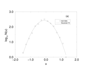
We apply histogram techniques to find the probability distribution of $u(t).$ Fig. 2(a) shows that $u(t)$ (Fig. 1(d)) is Gaussian distributed. Therefore, the signal in Fig. 1(c) is log-normally distributed. Since log-normal distributions often arise from underlying multiplicative processes, we study correlations in $u(t).$

The power spectrum of $u(t)$ cannot be computed using the fast Fourier transform (FFT) algorithms because the data are missing on up to 7% of all days. We calculate the power spectrum $P(f)$ of the sequence $u(t)$ using a Fourier transform algorithm that can correctly treat the “missing” data. The “Lomb normalized power spectrum” [6], $P(f)$ , often used when the data are unevenly sampled or missing, is shown in Figs. 2(b) and (c) on a double log scale. (The Lomb spectrum gives an estimate of the harmonic content of a data set for frequency $f$ that is based on a linear least-squares fitting to the function $A\sin(2\pi ft)+B\cos(2\pi ft)$ [6, 7].) We find prominent 1 y and 2 y spectral components in the data. This finding suggests that the fluctuations are due in part to environmental factors. Since the environment has “memory” (long-range correlated behavior), we next test for long-range correlations in the data. The linear behavior of the log-log plot of

P(f)\sim f^{-\beta}\;\;,

(2)

indicates the presence of scale invariant behavior. The scaling exponent $\beta\approx 0.7$ indicates that the data are long-range correlated, since the autocorrelation function decays in time with exponent $\gamma=1-\beta$ for $0<\beta<1.$ Note that $\beta=0$ for uncorrelated white noise and $\beta=1$ corresponds to $1/f$ -type noise. We have verified our finding of long-range correlations using other methods and find consistent results.

III Model

We model the long-term behavior of the activity concentration fluctuations. We first generate a sequence $w(t)$ of long-range correlated Gaussian noise with $\beta=0.7$ (the value of $\beta$ observed experimentally). We then exponentiate this sequence to obtain a second sequence $x(t)$ that is log-normally distributed as well as long-range correlated. The normalization of $x(t)$ is such that the mean and variance are fixed to be identical to those of the sequence $u(t)$ obtained from real data. Next, we multiply the sequence $x(t)$ by the exponential best fit function $C_{0}(t)$ found empirically, thereby obtaining the model sequence $C_{M}(t)$ (Fig. 2(d)). The model sequence $C_{M}(t)$ and the original data $C(t)$ are characterized by the same exponential trend, log-normal distribution, and power spectrum. The predicted activity concentrations never rise above 10^-2 mBq/m^-3 after 1998, even for extremely large fluctuations. The prediction is encouraging from a human health and environmental perspective, since this level is considered to be safe.

IV Discussion

The log-normal distribution [8] could be related [2] to local resuspension of the radionuclides by wind and transport from distant areas. Additional support for the possibility that local resuspension is the leading factor determining the observed fluctuation arises (i) from the presence of the pronounced 1 y spectral component and (ii) from the observed long-range correlations, as we next discuss:

(i)

A pronounced 1-year periodicity can be attributed to large-scale seasonal environmental changes, such as snow melting, as well as to human agricultural activity, such as plowing. Both yearly processes can release radioactive elements accumulated in soil.
(ii)

Long-range correlations with shorter characteristic times can be generated by large-scale atmospheric turbulence. It is possible that resuspension of radionuclides due to changing weather conditions [9] give rise to long-range correlated fluctuations around the exponentially decaying average activity concentrations, $C_{0}(t)$ . However, it is clear, that it is not only weather that is responsible for the observed long-range correlations in the activity levels. Ecosystems consist of a large number of reservoirs (e.g., forests, lakes, swamps and agricultural fields) of various sizes that can repeatedly absorb and release radionuclides into the environment [10]. It is well known since the works of Hurst [11] that the level of water in lakes is characterized by power law decaying fluctuations with the Hurst exponent $H\approx 0.7$ [11], The amount of radionuclides released in a unit of time should be proportional to the derivative of these fluctuations and hence should have a power spectrum scaling exponent $\beta=2H-1$ [12], which is in qualitative agreement with our measurements. The value of $\beta\approx 0.7$ found by us is larger than the value $0.4$ obtained from Hurst measurements and the discrepancy may be partially related to the fact that the high frequency part of the power spectrum (see Fig. 2(c)) has smaller slope $\beta\approx 0.5$ . Similar values of $\beta\approx 0.5$ as well as log-normal distributions of fluctuations were obtained for river discharges [13]. Moreover, the radioactive release is related not only to lakes but also to other parts of the ecosystem, which may have different Hurst exponents. Indeed, the influence of weather (and possibly forest fires) on monthly mean ¹³⁷Cs concentrations provides an illustration of how the ecosystem can absorb and release radionuclides [14]. The power law behavior of the power spectrum indicates that the temporal correlations decay as a power law $\sim t^{-\gamma}$ , with $\gamma=1-\beta$ [15]. Hence our analysis yields $\gamma=0.3$ . The model of wind resuspension used in [5] also predicted power law decaying correlations but with $\gamma=2/3$ , indicating a much faster decay than we observe. Indeed, such slowing down of the correlation decay with respect to the pure atmospheric activity is often observed in the the response of ecosystems such as forests and ground waters [13, 16].

V Conclusion

In summary, we have attempted to find a complete statistical description of the data. We have succeeded in quantifying both the probability distribution as well as the correlation properties of $C(t)$ —the two most fundamental statistical properties of time series. As with refs. [5, 17], the values obtained for the fitting parameters provide important information on the emission quantity and removal processes of radionuclides from the accident site. The differences between our results and those of [5, 17] may indicated the significant role of the ecosystems in the radionuclides resuspension. One important conclusion is that the observed long-range correlations are not solely due to the atmospheric turbulence but are strengthened by the accumulation of radionuclides by ecosystems, such as forests and ground waters.

Acknowledgments

We thank C. Argolo, M. Barbosa, T. Keitt, S. Lovejoy, M. L. Lyra, R. Mantegna, R. Nowak and T. J. P. Penna for discussions. We thank the Brazilian agency CNPq and NSF for support.

REFERENCES

[1] E. K. Garger, J. Aerosol Sci. 25, 754 (1994).
[2] E. K. Garger, V. A. Kashpur, B. I. Gurgula, H. G. Paretzke and J. Tschiersch, J. Aerosol Sci. 25, 767 (1994)
[3] USSR State Committee on the Utilization of Atomic Energy 1986, “The accident at the Chernobyl nuclear power plant and its consequences,” information compiled for the IAEA Experts Meeting August 25–29, Vienna (1986).
[4] Ilyin, L.A. and Pavlovskij, “Radiological consequences of the Chernobyl accident in the Soviet Union and measures taken to mitigate their impact.” IAEA Bulletin 4.
[5] Y. Hatano, N. Hatano, Atmospheric Environment 31, 2297 (1997).
[6] N. R. Lomb, Astrophysics and Space Science 39, 447 (1976).
[7] W. H. Press,, S. A. Teukolsky, W. T. Vetterling and B. P. Flannery, Numerical Recipes in C: the Art of Scientific Computing (Cambridge University Press, Cambridge, 1992).
[8] K. E. Bencala and J. H. Seinfeld, Atmos. Envir. 10, 941 (1976).
[9] E. Koscielny-Bunde, A. Bunde, S. Havlin, H. E. Roman, Y. Goldreich and H.-J. Schellnhuber, Phys. Rev. Lett. 81, 729 (1998).
[10] T. H. F. Allen and T. B. Starr, Hierarchy (Chicago University Press, Chicago, 1982).
[11] H. E. Hurst, R. P. Black and Y. M. Simaika, Long-Term Storage: An Experimental Study (Constable, London, 1965).
[12] T. Vicsek, M. Shlesinger and M. Matsushita, eds., Fractals in Natural Sciences, (World Scientific, Singapore, 1994).
[13] J. D. Pelletier and D. L. Turcotte, J. Hydrology 203, 198 (1997).
[14] E. K. Garger, F. O. Hoffman and K. M. Thiessen, Atmospheric Environment 31, 1647 (1997).
[15] C.-K.Peng et al, Phys. Rev. E 47, 3730 (1993).
[16] H. Lange, International Journal of Computing Anticipatory Systems 3, 169 (1999). See also H. Lange, http://www.interjournal.org, MS 250 (2000), http://www.bitoek.uni-bayreuth.de/ Holger.Lange/iccs2/cover.htm (preprint).
[17] Y. Hatano N. Hatano H. Amano T. Ueno A. K. Sukhoruchkin S. V. Kazakov Atmospheric Environment 32, 2587 (1998).

Refer to caption — FIG. 1.: (a) ¹³⁷Cs activity concentration $C(t)$ measured after the Chernobyl disaster as a function of time $t$ in days. (b) Semi-log plot of the data and the exponential best fit $C_{0}(t)\sim\exp[-t/677],$ obtained by regression (solid line). (c) Fluctuations after correcting for the exponential decay. The data $C(t)$ have been divided by the exponential fit $C_{0}(t)$ . (d) Logarithms $u(t)\equiv\log_{10}[C/C_{0}]$ of these data. The nonstationarity apparent to the naked eye in (a) appears eliminated in (c) and (d).