Collective modes in uniaxial incommensurate-commensurate systems
with the real order parameter

Abstract

The basic Landau model for uniaxial systems of the II class is nonintegrable, and allows for various stable and metastable periodic configurations, beside that representing the uniform (or dimerized) ordering. In the present paper we complete the analysis of this model by performing the second order variational procedure, and formulating the combined Floquet-Bloch approach to the ensuing nonstandard linear eigenvalue problem. This approach enables an analytic derivation of some general conclusions on the stability of particular states, and on the nature of accompanied collective excitations. Furthermore, we calculate numerically the spectra of collective modes for all states participating in the phase diagram, and analyze critical properties of Goldstone modes at all second order and first order transitions between disordered, uniform and periodic states. In particular it is shown that the Goldstone mode softens as the underlying soliton lattice becomes more and more dilute.

I Introduction

One of the most useful insights into the properties of stable and metastable ordered states in many body systems follows from the investigations of accompanying collective modes, excitations with a coherent participation of (semi)macroscopic number of particles. The attention is usually focused on the lowest branch in the spectrum. If it is of Goldstone type, i. e. gapless (e. g. acoustic) in the long wavelength limit ($k\rightarrow 0$), there is a continuous degeneracy in the characterization of ordered state, associated with the breaking of symmetry of the high temperature thermodynamic phase. Without the continuity in the degeneracy one has instead a finite gap at $k=0$.

Obvious extrinsic causes for the gap in the Goldstone mode are impurities, defects in the crystal structure, etc. Another cause for the gap is the presence of long range interactions [1]. We do not consider either of these mechanisms here, but remind that, as is well known in charge density wave materials [2, 3], they may play a decisive role in the collective dynamics of ordered state. Instead, we concentrate on the systems in which the above distinction regarding the degeneracy of ordered state(s) has its origin in short range interactions. Those are numerous materials that show one or more types of uniaxially modulated orderings with periodicities which may be commensurate or incommensurate with respect to the underlying crystal lattice [4, 5].

Let us at the beginning invoke some simple widely accepted conclusions, accumulated through intense theoretical and experimental investigations on these incommensurate-commensurate (IC) systems in last few decades. In an ideal case of sinusoidal modulation the spectrum of collective excitations contains two types of modes, phasons and amplitudons, representing linearized fluctuations of phase and amplitude of the order parameter respectively. While the amplitudon mode has a finite gap below the critical temperature, the phason mode is acoustic if the free energy of corresponding state does not depend on the relative phase of ordered modulation and crystal lattice. In other words one has the continuous degeneracy with respect to this relative phase. It is strictly fulfilled only if the modulation is incommensurate with respect to the periodicity of crystal lattice.

For commensurate modulations the free energy depends on the relative phase, as is easily seen already from the standard Landau expansions in which the lattice discreteness is taken into account by keeping a leading Umklapp contribution. Within this standard and frequently explored model [6, 7], which leads to the simple variational equation of sine-Gordon type, the phason mode acquires a gap which is finite only for the strict commensurate ordering, and diminishes rapidly (exponentially) as the order of commensurability increases. For other modulations, which may have the form of dilute soliton lattices, the Goldstone mode remains gapless, although among these modulations there are solutions with commensurate periodicities close to the exempted leading commensurability. In other words, within this model one does not distinguish between ”secondary” commensurate orderings and incommensurate orderings. This is the consequence of a crude simplification made by retaining only one Umklapp term in the free energy. The recent analysis shows that already after taking into account two leading Umklapp terms the phase diagram becomes qualitatively different [8, 9]. It contains a finite number of commensurate states, and shows a harmless staircase, i. e. a series of first order transitions between neighboring states. The Goldstone mode is then expected to have a finite gap for each state participating in the phase diagram.

The Landau models for the orderings with spatial modulations are generally justified providing the interactions responsible for their stabilization are weak enough, so that the variations of order parameter (defined with respect to the appropriately chosen star of wave vectors) are slow at the scale of lattice constant. Two crucial simplifications are then allowed, namely the gradient expansion and the perturbative treatment of lattice discreteness through the truncation of the sum of Umklapp contributions.

In the opposite regime of strong couplings the above spatial continuation is not allowed, and the lattice discreteness leads to qualitatively different properties of phase diagrams and related spectra of excitations, established by numerous analytical, and particularly numerical, studies of spin (e.g. Ising) [10, 11], displacive (e.g. Frenkel-Kontorova) [12], and electron-phonon (e.g. Holstein) [13, 14] discrete models. Characteristically for such models, either a finite, sometimes large, number of commensurate modulations in the cases of harmless staircase, or the infinity of them in the cases of complete devil’s staircases, can participate in the phase diagram. All commensurate states then have lowest branches of collective excitations with finite gaps in the limit $k\rightarrow 0$. We repeat that, while none of these possibilities can be reproduced by Landau model with one Umklapp term, the former harmless staircases with a finite number of commensurate states are realized already within extended Landau models with only two Umklapp terms taken into account [8, 9].

The analysis of Frenkel-Kontorova and Holstein models established also a new type of instability that involves incommensurate modulations, the so-called transition by breaking of analyticity [15]. Namely, by increasing the coupling constant [16], or by decreasing temperature  [17, 18], the smooth envelope of an incommensurate periodic modulation becomes nonanalytic. The free energy then depends nonanalytically on the relative phase of modulation and underlying lattice. As a consequence a finite gap opens in the Goldstone branch of collective excitations even for incommensurate modulations.

Already from the beginning of investigations on discrete models it was realized that the above complex features in phase diagrams and spectra of collective excitations have their origin in the nonintegrability of these models, i. e. in the nontrivial chaotic structures of corresponding phase spaces. In this respect it is important to emphasize that, either in their basic form or after the inclusion of further terms, Landau free energy expansions are as a rule the examples of nonintegrable functionals. For example, while the sine-Gordon model with one Umklapp term, as a basic model for class I of IC systems, is integrable, already the inclusion of another Umklapp term brings in the nonintegrability [8, 9].

The situation is even more intriguing for the class II, i. e. for IC materials with modulations having the period close or equal either to the original or to the dimerized unit cell of crystal lattice. There are numerical [19] and analytical [20] indications that already the minimal [21, 22], as well as slightly extended [23], models for this class are not integrable. The consequences of this nonintegrability on the phase diagram are discussed in detail in Ref. [20]. In particular, it is shown that, in addition to simple disordered, commensurate [i. e. (anti)ferro] and (almost) sinusoidal incommensurate states, included into previous analyses [22, 24, 23], the phase diagram contains also an enumerable family of metastable solutions with the periodic alternations of commensurate and incommensurate sinusoidal domains.

In the present work we calculate the spectrum of collective modes for stable and metastable states in systems of class II. The corresponding Landau model is particularly convenient for the discussion of questions raised in this Introduction, since it is nonintegrable, and, in addition, the accompanying phase diagram comprises both commensurate and incommensurate (meta)stable states. Our main aim is to investigate to what extent are the collective modes influenced by the nonintegrability of, here continuous, free energy functional. Furthermore, by analyzing Goldstone modes for the modulated states of the model under consideration [22, 23] we also resolve some controversies present in the literature [25, 26, 27, 28, 29] on its applicability in the description of incommensurate phases in systems of class II. The equivalent analysis for the class I, i. e. for the Landau model with two Umklapp terms, will be presented elsewhere [30].

The plan of the paper is as follows. The free energy functional for the class II is introduced in Sec. II. In Sec. III we perform the variational procedure up to the second order, taking care about some specific questions related to the thermodynamic minimization [31]. The linear eigenvalue problem associated to the second order variational procedure is discussed in Sec. IV. Here we encounter a generalized Hill problem, since the systems includes four coupled first order equations (in contrast to the standard cases with two equations), and furthermore, since we are looking for the collective modes of highly multiharmonic periodic states. We therefore do not follow a standard way, appropriate for simple sinusoidal incommensurate orderings, but develop for the first time a general formalism, applicable also to other types of Landau models. This formalism enables the determination of Floquet exponents, and of corresponding Bloch basis of eigenfunctions which we consider in Sec.V. The numerical results for the collective modes of all (meta)stable states appearing in the phase diagram are presented in Sec. VI. Concluding remarks along the lines specified in the previous paragraph are given in Sec. VII.

II Model

The free energy functional for the uniaxial incommensurate systems of class II is given by

$$\tilde{f}[\tilde{u}]=\frac{1}{2\tilde{L}}\int_{-\tilde{L}}^{\tilde{L}}\left[d\left(\frac{d^{2}\tilde{u}}{d\tilde{z}^{2}}\right)^{2}+c\left(\frac{d\tilde{u}}{d\tilde{z}}\right)^{2}+a\tilde{u}^{2}+{\scriptstyle\frac{1}{2}}b\tilde{u}^{4}\right]d\tilde{z}$$ (1)

where $\tilde{u}$ represents the real order parameter and $\tilde{L}$ is the length of the system. This functional is the simplest (minimal) Landau expansion for the systems with minima of free energy density in the reciprocal space close to the center of Brillouin zone, or to the part of its border perpendicular to the uniaxial direction. Then $c<0$, and one has to add a highly nontrivial term with the second derivative of $\tilde{u}$ (and presumably positive coefficient $d$) in order to ensure the boundness of Landau expansion in the reciprocal space. The rest of the expansion (1) is standard, with $b>0$, and $a$ becoming negative below the critical temperature of the transition from disordered to uniform (ferro) or dimerized (antiferro) phase. We limit the further analysis to the most interesting regime characterized by $c<0$. It includes the incommensurate ordering and the transition to the commensurate ordering (but does not include the transition from disordered to commensurate state which takes place for $c>0$) [21, 22]. In this regime the useful dimensionless quantities are

$$z=\sqrt{-\frac{c}{d}}\tilde{z},\,\,\,\ L=\sqrt{-\frac{c}{d}}\tilde{L},\,\,\,\ u(z)=-\frac{\sqrt{bd}}{c}\tilde{u}(\tilde{z}),\,\,\,\ f[u]=\frac{bd^{2}}{c^{4}}\tilde{f}[\tilde{u}].$$ (2)

The model (1) can be now represented as the one-parameter problem,

$$f[u]=\frac{1}{2L}\int_{-L}^{L}\left[\left(\frac{d^{2}u}{dz^{2}}\right)^{2}-\left(\frac{du}{dz}\right)^{2}+\lambda\,u^{2}+{\scriptstyle\frac{1}{2}}u^{4}\right]dz,$$ (3)

with $\lambda\equiv ad/c^{2}$. The parameterization of the phase diagram in the regime $c<0$ is thus very simple, since all relationships between different (meta)stable states (like phase transitions, ranges of coexistence of two or more states, etc) can be presented in the one-dimensional $\lambda$-space. The knowledge of the actual dependence of this parameter, as well as of the scales which enter into the reduced quantities (2), on the original physical parameters, in particular on temperature, goes together with the specification of microscopic background behind the phenomenological free energy (1). This is a necessary step in any comparison of phase diagram for the model (3) with experimental data for a given material.

In the previous works [19, 20] on the functional (3) we have determined thermodynamically stable states, i. e. its local minima, without taking into considerations statistical fluctuations outside these minima. This mean-field type of approximation is inappropriate for (quasi) one-dimensional systems. It is however usually sufficient for three-dimensional uniaxial systems with strong enough couplings in the perpendicular directions, on which we concentrate here.

The thermodynamic extremalization of functional (3) consists of the standard variational procedure that is equivalent to the classical mechanical one and leads to the corresponding Euler-Lagrange (EL) equation

$$\frac{d^{4}u}{dz^{4}}+\,\frac{d^{2}u}{dz^{2}}+\lambda\,u+u^{3}=0,$$ (4)

and of the extremalization that involves boundary conditions or some equivalent set of parameters. The general procedure that carefully takes into account the latter aspect is proposed in Ref. [31]. The most interesting result of this approach is obtained for the functional with the kernel that is not explicitly $z$-dependent. Then the relation

$$F=-H,$$ (5)

holds for each thermodynamic extremum $u_{0}(z)$. Here $F$ is the corresponding averaged free energy, and $H$ is the integral constant of the problem (4) which corresponds to the Hamiltonian in classical mechanics.

Early considerations of the model (1) led to the suggestion that the mean-field phase diagram [21, 22, 24, 32, 33] contains only disordered [$u_{d}(z)=0$], commensurate [$u_{c}(z)=\pm\sqrt{-\lambda}$], and (almost) sinusoidal [$u_{s}(z)\approx 2/\sqrt{3}(\sqrt{1/4-\lambda})\sin{(z/\sqrt{2})}$] incommensurate orderings. The commensurate state is thermodynamically stable for $\lambda<-1/8$ (and for $a<0$ in the range $c>0$). The incommensurate state is stable in the range $-2<\lambda<\lambda_{id}=1/4$, while the first order phase transition between the commensurate and the incommensurate states occurs at $\lambda_{ic}=-1.112$. The more precise values, obtained after taking into account corrections from higher harmonics in the sinusoidal ordering [20], are $-1.835<\lambda<\lambda_{id}$ and $\lambda_{ic}=-1.177$. Also, the wave number of this ordering, $q$, slightly deviates from $1/\sqrt{2}$ [i. e. from $\sqrt{-c/(2d)}$ in the original parameters of Eq. (1)] as one approaches the left edge of instability, $\lambda\rightarrow-1.835$.

While by above solutions of EL equation (4) one exhausts all absolute minima of the free energy (1), the more involved numerical analysis [19, 20] showed the existence of an enumerable series of periodic solutions which are metastable in finite ranges of the parameter $\lambda$. The corresponding phase diagram is shown in Fig. 1 in which we ascribe to various solutions symbolic words introduced in Ref. [20]. By their physical content the metastable solutions from Fig. 1 represent periodic trains of successive sinusoidal and uniform segments (see Fig. 1 in [20]), and, as domain patterns, complete in a natural way, as an inherent outcome of nonintegrable model (1), the phase diagram in the range of coexistence of two corresponding basic types of orderings.

III Second order variational procedure

The question on which we concentrate now is the thermodynamic stability of a given state $u(z)$ which is a solution of EL equation (4) and fulfills additional conditions of Ref. [31]. To this end we have to go beyond the linear terms in the extremalization procedure. Let us therefore at first extend the standard variational procedure to the second order. Later on we shall shortly consider the conditions which follow from the minimization of boundary conditions.

Let $\eta(z)$ be the infinitesimal variation with respect to $u(z)$, obeying usual conditions at the boundaries $z=0$ and $z=L$,

$$\eta(z=0)=\eta(z=L)=\eta^{\prime}(z=0)=\eta^{\prime}(z=L)=0.$$ (6)

After performing standard partial integrations,

$$\frac{1}{L}\int_{0}^{L}(\eta^{\prime})^{2}dz = \frac{1}{L}\eta^{\prime}\eta\arrowvert_{0}^{L}-\frac{1}{L}\int_{0}^{L}\eta^{\prime\prime}\eta dz,$$ (7)

$$\frac{1}{L}\int_{0}^{L}(\eta^{\prime\prime})^{2}dz = \frac{1}{L}\eta^{\prime\prime}\eta^{\prime}\arrowvert_{0}^{L}-\frac{1}{L}\eta^{\prime\prime\prime}\eta\arrowvert_{0}^{L}+\frac{1}{L}\int_{0}^{L}\eta^{IV}\eta dz,$$ (8)

the quadratic contribution to the corresponding variation of free energy functional (3) can be expressed in the form

$$\delta^{2}f\equiv f[u+\eta]-f[u]=\frac{1}{L}\int_{0}^{L}dz\eta{\cal D}\eta,$$ (9)

with

$${\cal D}\equiv\frac{d^{4}}{dz^{4}}+\frac{d^{2}}{dz^{2}}+\lambda+3u^{2}.$$ (10)

The linear differential operator (10) defines the eigenvalue problem

$${\cal D}\eta_{\Lambda}\equiv\eta^{\prime\prime\prime\prime}_{\Lambda}(z)+\eta^{\prime\prime}_{\Lambda}(z)+\left[\lambda+3u^{2}(z)\right]\eta_{\Lambda}(z)=\Lambda\eta_{\Lambda}(z),$$ (11)

with the boundary conditions for $\eta(z)$ specified by Eq. (6). The necessary condition for the thermodynamic stability of solution $u(z)$ is given by the requirement that the spectrum $\Lambda$ is non-negative for all normalizable solutions $\eta_{\Lambda}(z)$ of the problem (10,6).

Since the above procedure strictly respects the boundary conditions (6), it is entirely equivalent to that usually used in classical mechanics. As a consequence the obtained condition for the stability of a given solution $u(z)$ holds for any value of the sample length $L$. However, neither the extremal solution $u(z)$ of EL equation (4), nor the corresponding conditions of thermodynamic stability, should be sensitive to the conditions imposed on the sample surfaces in the physically relevant thermodynamic limit $L\rightarrow\infty$. Therefore the stability condition can be generalized in this limit. In particular, we may ignore the boundary conditions (6), and perform the variational procedure for any infinitesimal variation $\eta(z)$, noting, for later purposes, that the requirement of infinitesimality excludes variations $\eta(z)$ which would scale as $|z|^{\beta}$ with $\beta>0$.

Performing the same steps as before, but now with neglected surface terms in Eqs. (8) (which scale as $1/L$), we come again to the linear eigenvalue problem (11), but without a specification on boundary conditions. This means that any complete set of eigenfunctions $\eta_{\Lambda}(z)$ with the eigenvalues $\Lambda$ [which are themselves characterized solely by the linear differential equation (11)] can be used in the representation of a given variation $\eta(z)$, and in the corresponding diagonal representation of the free energy (9). The condition ${\Lambda}\geq 0$ thus guarantees the thermodynamic stability of the solution $u(z)$ with respect to any infinitesimal variation, provided the system has the well-defined thermodynamic limit as specified above. We note that by this relaxation of boundary conditions (6) we extend the standard ”classical mechanical” second order variational procedure by including a part of, but still not all, ”thermodynamic” variations. The discussion of this question in Appendix A suggests that the criterion of thermodynamical stability is probably entirely covered by the eigenvalue problem (11).

The concise definition of the thermodynamical stability, i. e. of the stability of any (absolutely stable or metastable) local minimum of thermodynamic functional with respect to small fluctuations, is thus:

• A given solution of EL equation (4) is thermodynamically stable if and only if all solutions of Eq.(11) for any $\Lambda<0$ are non-normalizable.

For later purpose it is appropriate to introduce here also the concept of orbital stability, relevant for the behavior of particular solutions in the phase space:

• A given solution $u(z)$ of EL equation (4) is orbitally stable if and only if all solutions of Eq.(11) for $\Lambda=0$ are normalizable.

In the next section the above definitions will be used in the study of stability of homogeneous and periodic configurations $u(z)$. The crucial assumption in this respect is that the solutions of Eq.(11) smoothly depend on both parameters $\lambda$ and $\Lambda$.

Before embarking into the calculation of the spectrum of eigenvalue problem (11), we invoke its general property which follows from the fact that the density of free energy functional (3) does not depend explicitly on the spatial coordinate $z$. Then there exists a normalizable solution of equation (11) with $\Lambda=0$, namely $\eta_{0}(z)\propto u^{\prime}(z)$. This is the Goldstone mode that follows from the translational invariance of free energy functional (3), by which $u(z+z_{0})$ with arbitrary $z_{0}$ is the solution of EL equation (4) if $u(z)$ is its solution. We note that Eq.(11) then has, together with the above Goldstone mode, another solution of the form $\eta_{1}(z)=w(z)+z\cdot u^{\prime}(z)$, where $w(z)$ is some periodic function of the same period as that of the Goldstone mode. Although $\eta_{1}(z)$ is non-normalizable i.e. its norm grows as a power of $L$, we consider this non-normalizability as marginal. The power law growth of a solution of Eq.(11) is much easier to control than possible exponential growth of the remaining solutions, if there are any. For special values of the parameter $\lambda$ figuring in Eq.(11) with $\Lambda=0$ the only normalizable solution is the Goldstone mode $u^{\prime}(z)$, while other solutions have a power law growth in $z$, $z^{n}u^{\prime}(z)$ with $n\leq 3$. These special values of $\lambda$ denote the edges of thermodynamical metastability of the corresponding configuration $u(z)$.

IV Floquet theory

The analysis of the eigenvalue problem (11) with periodic functions $u(z)$ is based on general Floquet and Bloch theorems for linear differential equations with periodic coefficients. It will be performed in two stages, covered by this and the next section. The aim of the first one, based on the Floquet’s approach, is to answer the question: Whether there exists a normalizable solution $\eta_{\Lambda}(z)$ for a given value of $\Lambda$? In the second stage we calculate the set of values $\Lambda$ for which normalizable solutions exist, i.e. the spectrum of collective modes, by using the Bloch’s wave number representation.

We begin by showing that the set of values of $\Lambda$ for which the corresponding normalizable solutions $\eta_{\Lambda}(z)$ may exist is bounded from below. To this end let us rewrite Eq. (11) in the form

$${\tilde{\cal D}}^{2}\eta_{\Lambda}(z)+3\,u(z)^{2}\eta_{\Lambda}(z)=\left(\Lambda+\frac{1}{4}-\lambda\right)\eta_{\Lambda}(z)\,\,\,,\,\,\,{\tilde{\cal D}}\equiv\frac{d^{2}}{dz^{2}}+\frac{1}{2},$$ (12)

and introduce the norm of the function $\eta_{\Lambda}(z)$,

$$\parallel\eta_{\Lambda}\parallel^{2}\equiv\left<\eta_{\Lambda}^{*}\eta_{\Lambda}\right>=\frac{1}{L}\int_{0}^{L}\eta_{\Lambda}(z)^{*}\eta_{\Lambda}(z)dz.$$ (13)

After multiplying Eq. (12) by $\eta_{\Lambda}^{*}(z)$ and integrating with respect to $z$ we get

$$\parallel{\tilde{\cal D}}\eta_{\Lambda}(z)\parallel^{2}+3\,\parallel u(z)\eta_{\Lambda}(z)\parallel^{2}=\left(\Lambda+\frac{1}{4}-\lambda\right)\parallel\eta_{\Lambda}(z)\parallel^{2}.$$ (14)

Here it is taken into account that the operator ${\tilde{\cal D}}$ is hermitean and the function $u(z)$ is real. Since the left-hand side of Eq. (14) is strictly positive, we conclude that

$$\Lambda\geq\Lambda_{min}=\lambda-\frac{1}{4}$$ (15)

for each $\Lambda$ for which the the norm (13) of the function $\eta_{\Lambda}(z)$ exists. In particular, this means that it is sufficient to reduce a (numerical) analysis of the thermodynamic stability of a given configuration $u(z)$ to the search for the normalizable eigenfunctions $\eta_{\Lambda}(z)$ in the finite interval of $\Lambda$, $\Lambda_{min}\leq\Lambda<0$.

Before considering Eq. (11) with the general periodic function $u(z)$, let us establish the criterion for the thermodynamic stability of the particular homogeneous (ferro or antiferro) solution $u_{c}(z)=\pm\sqrt{-\lambda}$ of EL equation (4). Then Eq. (11) reduces to the linear differential equation with constant coefficients, so that the normalizable eigenfunctions must have the form $\eta(z)\propto e^{ikz}$ with real values of the wave number $k$. The corresponding eigenvalues $\Lambda$ are given by

$$\Lambda=k^{4}-k^{2}-2\lambda\,\,\,,\,\,\,\lambda<0.$$ (16)

It follows that the homogeneous configuration $u_{c}(z)=\pm\sqrt{-\lambda}$ is stable, i.e. that $\Lambda>0$ for any $k$, provided that $\lambda<-1/8$. Note that the latter inequality is just the condition of orbital instability of the homogeneous solution. Namely, the linearization of the EL equation with respect to this solution leads to the linear equation

$$\theta^{\prime\prime\prime\prime}+\theta^{\prime\prime}-2\lambda\theta=0,$$ (17)

which has normalizable solutions $\theta(z)$ only for $\lambda>-1/8$. Thus, we see that in this simple case the thermodynamic stability excludes the orbital stability, and vice versa, and that two stabilities ”meet” each other in one point, $\lambda=-1/8$.

A General Floquet’s procedure

In order to apply the well-known Floquet’s procedure [34] to Eq. (11) with a general periodic function $u(z)$, we rewrite this equation in the matrix form

$$\frac{d{\bf\Theta}(z)}{dz}={\bf A}(z;\lambda,\Lambda){\bf\Theta}(z),$$ (18)

where ${\bf\Theta(z)}\equiv[\eta(z),\eta^{\prime}(z),\eta^{\prime\prime}(z),\eta^{\prime\prime\prime}(z)]^{T}$, and the matrix $\mbox{{\bf A}}(z;\lambda,\Lambda)$ is given by

$$\mbox{{\bf A}}(z)=\left(\begin{array}[]{cccc}0&1&0&0\\ 0&0&1&0\\ 0&0&0&1\\ \Lambda-\lambda-3\,u(z)^{2}&0&-1&0\end{array}\right).$$ (19)

The system of linear equations (18) has four linearly independent solutions, ${\bf\Theta}_{i}(z),i=1,...,4$. They form the fundamental matrix

$$\mbox{{\bf F}}(z)=\left[{\bf\Theta}_{1}(z),{\bf\Theta}_{2}(z),{\bf\Theta}_{3}(z),{\bf\Theta}_{4}(z)\right],$$ (20)

which is obviously the solution of equation

$$\frac{d\mbox{{\bf F}}(z)}{dz}=\mbox{{\bf A}}(z;\lambda,\Lambda)\mbox{{\bf F}}(z).$$ (21)

Without reducing generality we can always choose such initial conditions at $z=0$ that $\mbox{{\bf F}}(0)=\mbox{{\bf I}}$, where I is the identity matrix.

The Floquet’s theorem states that whenever the matrix $\mbox{{\bf A}}(z;\lambda,\Lambda)$ is a periodic function of variable $z$ with a period $P$, the fundamental matrix has the form

$$\mbox{{\bf F}}(z)=\mbox{{\bf G}}(z)\mbox{e}^{{\bf\Sigma}z},$$ (22)

where $\mbox{{\bf G}}(z)$ is a matrix which varies periodically with $z$, $\mbox{{\bf G}}(z+P)=\mbox{{\bf G}}(z)$, and ${\bf\Sigma}$ is a constant matrix. Due to the periodicity of matrix $\mbox{{\bf G}}(x)$ and the initial condition $\mbox{{\bf G}}(0)=\mbox{{\bf I}}$, the matrix ${\bf\Sigma}$ can be expressed in the form

$${\bf\Sigma}=\frac{1}{P}\ln\mbox{{\bf F}}(P).$$ (23)

The matrix ${\bf F}(P)$ is called the monodromy matrix. The eigenvalues of ${\bf\Sigma}$, $\sigma_{i}$ are Floquet’s exponents and the eigenvalues of monodromy matrix $\mbox{{\bf F}}(P)$, $\rho_{i}$, are Floquet’s multipliers. Put in other words, Floquet’s theorem states that for each Floquet multiplier $\rho_{i}$ there exists a solution ${\bf\Theta}_{i}(z)$ of Eq. (18) with the property

$${\bf\Theta}_{i}(z+P)=\rho{\bf\Theta}_{i}(z).$$ (24)

Floquet multipliers $\rho_{i}$ are in general complex numbers. For a normalizable solution ${\bf\Theta}_{i}(z)$ the Floquet multiplier $\rho_{i}$ lies on the unit circle in the complex $\rho$-plane, and the corresponding Floquet exponent $\sigma_{i}$ is imaginary.

B Poincaré-Lyapunov theorem

The problem (18) has an additional important property. After the linear transformation ${\bf Z}(z)\equiv[Z_{1}(z),Z_{2}(z),Z_{3}(z),Z_{4}(z)]^{T}={\bf T}{\bf\Theta}(z)$, defined by

$$Z_{1}=\eta(z)\,\,,\,\,Z_{2}=\eta^{\prime\prime}(z)\,\,,\,\,Z_{3}=2(\eta^{\prime}(z)+\eta^{\prime\prime\prime}(z))\,\,,\,\,Z_{4}=2\eta^{\prime}(z),$$ (25)

i. e. by

$$\mbox{{\bf T}}(z)=\left(\begin{array}[]{cccc}1&0&0&0\\ 0&0&1&0\\ 0&2&0&2\\ 0&2&0&0\end{array}\right),$$ (26)

Eq. (18) is transformed into the equation

$$\frac{d\mbox{{\bf Z}}(z)}{dz}=\mbox{{\bf J H}}(z;\lambda,\Lambda)\mbox{{\bf Z}}(z),$$ (27)

with

$$\mbox{{\bf H}}(z)=\left(\begin{array}[]{cccc}-2(\lambda-\Lambda+3\,v_{0}(z)^{2})&0&0&0\\ 0&2&0&0\\ 0&0&0&-\frac{1}{2}\\ 0&0&-\frac{1}{2}&\frac{1}{2}\end{array}\right)\,\,,\,\,\mbox{{\bf J}}=\left(\begin{array}[]{cccc}0&0&-1&0\\ 0&0&0&-1\\ 1&0&0&0\\ 0&1&0&0\end{array}\right).$$ (28)

The problem (27) has the Hamiltonian form, characterized by the hermitean matrix H and the simplectic matrix J (i.e. J is antisymmetric and has the property $\mbox{{\bf J}}^{2}=-\mbox{{\bf I}}$). The Poincaré-Lyapunov (PL) theorem [35] for such problems states that the corresponding fundamental matrix, ${\bf\Phi}(z)$, satisfies the relation

$${\bf\Phi}^{T}(z){\bf J}{\bf\Phi}(z)={\bf\Phi}^{T}(0){\bf J}{\bf\Phi}(0).$$ (29)

In other words, ${\bf\Phi}^{T}(z){\bf J}{\bf\Phi}(z)$ is the ”integral of motion” for the Hamiltonian problem (27). This theorem can be easily checked by differentiating the relation (29) with respect to $z$, and taking into account Eq. (27). Since ${\bf\Phi}(z)=\mbox{{\bf T}}\mbox{{\bf F}}(z)$, and the matrix $\mbox{{\bf T}}^{T}\mbox{{\bf J}}\mbox{{\bf T}}\equiv\mbox{{\bf J}}_{1}$ is also simplectic, it follows that

$${\bf F}^{T}(z){\bf J}_{1}{\bf F}(z)={\bf F}^{T}(0){\bf J}_{1}{\bf F}(0)={\bf J}_{1},$$ (30)

i.e. the PL theorem holds for our original fundamental matrix $\mbox{{\bf F}}(z)$ as well.

From the relation (30) it follows that the matrices $\mbox{{\bf F}}^{T}(z)$ and $\mbox{{\bf F}}^{-1}(z)$ are similar [$\mbox{{\bf F}}^{T}(z)=\mbox{{\bf J}}_{1}\mbox{{\bf F}}^{-1}(z)\mbox{{\bf J}}_{1}^{-1}$]. Thus, if $\rho_{1}\equiv\rho$ is the Floquet multiplier of $\mbox{{\bf F}}(P)$, then $\rho^{-1}$ is also its Floquet multiplier. Furthermore, since in our example the matrix $\mbox{{\bf F}}(P)$ is real, it follows that $\rho^{*}$ and $\rho^{*-1}$ are Floquet multipliers as well. These simple relations link four Floquet multipliers of the problem (18) for any periodic solution of EL equation (4) and for any value of parameter $\lambda$. The corresponding three possible types of distributions of Floquet multipliers in the complex $\rho$-plane are shown in Fig. 2. Floquet multipliers are either complex (a) or real. In the latter case two pairs generally have different values and may be of the same (b) or opposite (c) signs. Fig. 2 does not include the situations with existing collective modes, i. e. when one or two pairs of solutions are normalizable, and the corresponding Floquet multipliers are on the unit circle.

Four Floquet multipliers of the problem (18) can be represented as roots of a polynomial function of fourth order. Since, due to the PL theorem, $\rho,\rho^{-1},\rho^{*}$ and $\rho^{*-1}$ are all roots of such function, its general form is

$$P_{4}(\rho)=\rho^{4}+a(\lambda,\Lambda)\left(\rho^{3}+\rho\right)+b(\lambda,\Lambda)\rho^{2}+1,$$ (31)

where $a(\lambda,\Lambda)$ and $b(\lambda,\Lambda)$ are, for a given periodic function $u(z)$, some smooth real functions of parameters $\lambda$ and $\Lambda$ from the matrix (19).

C Scenarios of thermodynamic (in)stabilities

Having recapitulated the Floquet theory for the Hamiltonian linear problem (18), we address the problem of thermodynamical stability for a given periodic configuration $u(z)$. We start by noting that Eqs. (18), (19) and (31) enable some general conclusions about the dependence of the positions of Floquet multipliers in the complex plane on the parameters $\lambda$ and $\Lambda$. At first, since $\rho=0$ cannot be the root of $P_{4}(\rho)$, it follows that by changing continuously $\lambda$ and $\Lambda$ one can come from the distributions (a) or (b) to the distribution (c) in Fig. 2 only by passing through the unit circle. Next, it is easy to determine the positions of Floquet multipliers in the limits $\Lambda\rightarrow-\infty$ and $\Lambda\rightarrow\infty$, since then we may neglect $\lambda$ and $u^{2}(z)$ with respect to $\Lambda$ in the polynomial matrix element of the matrix ${\bf A}$ (19) [still keeping in mind that $u(z)$ defines the period $P$ which enters into the definition (23)].

In the former limit $\Lambda\rightarrow-\infty$ the Floquet multipliers are given by

$$\rho_{n}=\mbox{e}^{k_{n}P}\,\,,\,\,k_{n}=\mid\Lambda\mid^{\frac{1}{4}}\mbox{e}^{i(2n+1)\frac{\pi}{4}}\,\,,\,\,n=0,1,2,3\,$$ (32)

i.e. the distribution from Fig. 2(a) is realized. Note that for $\Lambda<\Lambda_{min}$ this distribution cannot pass to that from Fig. 2(c), since in this range of values of $\Lambda$ the unit circle cannot be crossed because the problem (18) does not have normalizable solutions.

In the limit $\Lambda\rightarrow\infty$ the Floquet multipliers are given by

$$\rho_{1}=\rho_{2}^{-1}=\mbox{e}^{\Lambda^{\frac{1}{4}}P}\,\,\,\,,\,\,\,\,\rho_{3}=\rho_{4}^{-1}=\mbox{e}^{i\Lambda^{\frac{1}{4}}P}\,\,.$$ (33)

As is seen in Fig. 3, one then has one pair of normalizable and one pair of non-normalizable solutions.

From the other side, at $\Lambda=0$ one particular Floquet multiplier has the value $\rho=1$, and corresponds to the already mentioned Goldstone mode. It has to be at least doubly degenerate, since otherwise the remaining three multipliers could not have symmetric positions required by the PL theorem. Possible distributions of Floquet multipliers for $\Lambda=0$ are shown in Fig. 4. Aside from the possibility that the degeneracy of the Goldstone mode is complete and all four multipliers are at $\rho=1$ (a), one may have the remaining two multipliers either on the real axis (b,c), or on the unit circle (d).

Taking into account the above conclusions, we are now able to list possible scenarios of thermodynamic (in)stabilities for the periodic solutions of Eqs. (4,5).

1. The solution $u(z)$ is unstable for a given value of $\lambda$ if by increasing $\Lambda$ from $\Lambda_{min}=\lambda-1/4$ the Floquet multipliers from the distribution (a) or (b) of Fig. 2 move in such a way to come to the unit circle for some value of $\Lambda$ in the interval $(\lambda-1/4,0)$.

2. If the solution $u(z)$ is thermodynamically stable, the Floquet multipliers for $\lambda-1/4<\Lambda<0$ are defined either by one complex number not lying on the unit circle (Fig. 2a), or by two real numbers of the same sign ($r_{1},r_{2}$) and their reciprocals (Fig. 2b). The latter case has to be realized as $\Lambda\rightarrow 0$ from below, since only distributions (b) and (c) from Fig. 4 represent the Goldstone mode for a thermodynamically stable configuration. Thus, at some negative value of $\Lambda$ the distribution from Fig. 2a has to reduce to the double degenerate Floquet multiplier at the real axis ($r_{1}=r_{2}$), which then evolves into the distribution from Fig. 2b.

3. For special value(s) of control parameter ($\lambda=\lambda_{c}$) the thermodynamic instability of $u(z)$ proceeds in a particular way, realized when all four complex Floquet multipliers approach together the point $\rho_{0}=1$ as $\Lambda$ tends to zero from below. The Goldstone mode is then completely degenerate (Fig. 4a). Putting in another way, such instability occurs when the points $r$ and $r^{-1}$ in Fig.4b tend towards $\rho_{0}=1$ as $\lambda\rightarrow\lambda_{c}$. Note that the distribution of Floquet multipliers from Fig. 4c means that the instability, i.e. the crossing of Floquet multipliers with the unit circle, takes place at some negative value of $\Lambda$. Also, the distribution from Fig. 4d signifies that the remaining non-Goldstone mode is unstable in a finite interval of values of $\Lambda$, starting at some negative value of $\Lambda$.

V Bloch theory

In order to determine normalizable solutions of Eq. (18) with $\Lambda\geq 0$, i.e. the collective modes for given periodic configuration $u(z)$ with the period $P=2\pi/Q$, we profit from the freedom in choosing boundary conditions for the solutions $\eta(z)$, and specify periodic (Born - von Karman) ones. By this we chose the Bloch representation,

$$\eta_{k}(z)=e^{ikz}\Psi_{k}(z),\,\,\,\,\,\,\,\,\Psi_{k}\left(z+\frac{2\pi}{Q}\right)=\Psi_{k}(z),$$ (34)

where $k$ is the Bloch wave number limited to the I Brillouin zone ($-Q/2\leq k\leq Q/2$). The differential equation for the periodic function $\Psi_{k}(z)$ reads

$$\frac{d^{4}\Psi_{k}(z)}{dz^{4}}+4ik\frac{d^{3}\Psi_{k}(z)}{dz^{3}}+(1-6k^{2})\frac{d^{2}\Psi_{k}(z)}{dz^{2}}+2ik(1-2k^{2})\frac{d\Psi_{k}(z)}{dz}+$$ (35)

$$+\left[k^{4}-k^{2}+\lambda+3u(z)^{2}\right]\Psi_{k}(z)=\Lambda(k)\Psi_{k}(z),$$ (36)

and the normalizability condition is

$$\frac{Q}{2\pi}\int_{0}^{\frac{2\pi}{Q}}\Psi_{k}^{*}(z)\Psi_{k}(z)dz=1.$$ (37)

The dependence $\Lambda(k)$, i. e. the spectrum of eigenvalue problem (11), follows from Eqs. (36, 37). Since $k$ is quasi-continuous in the limit $L\rightarrow\infty$, this spectrum is for a stable configuration $u(z)$ composed of non-negative bands. The corresponding Bloch functions $\eta_{n,k}(z)$, where $n$ enumerates bands, represent a complete orthonormal set of functions for the problem (11).

From expressions (24) and (34) it follows that the Floquet multiplier for the Bloch function $\eta_{k}(z)$ is given by $\rho=\mbox{e}^{ikP}$. The polynomial function (31) then has the form

$$P_{4}(\rho)=\left(\rho-\mbox{e}^{ikP}\right)\left(\rho-\mbox{e}^{-ikP}\right)\left[\rho^{2}+c_{2}(\lambda,\Lambda)\rho+1\right]\,,$$ (38)

where $c_{2}(\lambda,\Lambda)$ is some coefficient. Comparing two representations for $P_{4}(\rho)$ we conclude that the coefficients from the expressions (31) and (38) are linked by relations

$$a(\lambda,\Lambda)=c_{2}(\lambda,\Lambda)-2\cos(kP)\,,\,\,\,\,\,\,\,\,\,b(\lambda,\Lambda)=2-2c_{2}(\lambda,\Lambda)\cos(kP)\,,$$ (39)

i. e. that the eigenvalue $\Lambda$ depends on the wave number $k$ only through the function $\cos(kP)$. This in particular means that for each band $\Lambda(k)$ we have $\Lambda(-k)=\Lambda(k)$. This is consistent with the symmetry of Eq. (36). Furthermore $\Lambda(k+\frac{2\pi}{P})=\Lambda(k)$, in accordance with the reduction of wave numbers in (34) to the I Brillouin zone.

The representation (34) is particularly convenient for the analytical discussion of long wavelength limit $k\rightarrow 0$ for the Goldstone mode for which $\Lambda(k=0)=0$ and $\Psi_{k=0}(z)=u^{\prime}(z)$. To this end we insert the Taylor expansions for small $k$,

$$\Psi_{k}(z)=u^{\prime}(z)+k\Psi_{1}(z)+k^{2}\Psi_{2}(z)+...\,\,\,,\,\,\,\Lambda(k)=k^{2}\Lambda_{2}+k^{4}\Lambda_{4}+...,$$ (40)

into Eq.( 36). The requirement that the coefficients in front of leading powers, $k$ and $k^{2}$, vanish then leads to the equations

$$\left(\tilde{\cal{D}}^{2}+\lambda-\frac{1}{4}+3u^{2}\right)\Psi_{1}=-2i\left(2u^{\prime\prime\prime\prime}+u^{\prime\prime}\right)\,\,,$$ (41)

and

$$\left(\tilde{\cal{D}}^{2}+\lambda-\frac{1}{4}+3u^{2}\right)\Psi_{2}=(\Lambda_{2}+1)u^{\prime}+6u^{\prime\prime\prime}-2i(2\Psi_{1}^{\prime\prime\prime}+\Psi_{1}^{\prime}),$$ (42)

with the operator $\tilde{\cal{D}}$ given by Eq. (12). After multiplying equation (42) by $v^{\prime}$, integrating with respect to $z$, using the fact that $u^{\prime}$ is the Goldstone mode, and inserting $2u^{\prime\prime\prime\prime}+u^{\prime\prime}$ from Eq. (41), we get the expression for the coefficient $\Lambda_{2}$,

$$\Lambda_{2}=-1+6\frac{\left<u^{\prime\prime 2}\right>}{\left<u^{\prime 2}\right>}-\frac{\left<\Psi_{1}^{*}\left(\tilde{\cal{D}}^{2}+\lambda-\frac{1}{4}+3u^{2}\right)\Psi_{1}\right>}{\left<u^{\prime 2}\right>},$$ (43)

where $\left<...\right>$ stands for the spatial integration, like in Eq. (13). However, the general thermodynamic condition (5) for the functional  (1) reads [31]

$$\frac{\left<u^{\prime\prime 2}\right>}{\left<u^{\prime 2}\right>}=\frac{1}{2}\,\,,$$ (44)

so that Eq. (43) can be written in a more transparent way,

$$\Lambda_{2}=2-F_{2}\left[u(z)\right]\,\,.$$ (45)

Here we introduce the functional

$$F_{2}\left[u(z)\right]=\frac{\left<\Psi_{1}^{*}\left(\tilde{\cal{D}}^{2}+\lambda-\frac{1}{4}+3u^{2}\right)\Psi_{1}\right>}{\left<u^{\prime 2}\right>}.$$ (46)

Since the operator figuring in this equation just defines the eigenvalue problem (11,12), it is clear that the functional $F_{2}\left[u(z)\right]$ is positive definite for any thermodynamically stable configuration $u(z)$. This has two consequences.

Firstly, the common upper limit of the velocity of Goldstone mode, $v_{G}=\sqrt{\Lambda_{2}}$, for all thermodynamically stable periodic states is $v_{G,M}=\sqrt{2}$. The velocity $v_{G}$ for a given (meta) stable state has the maximum value $v_{G,max}\leq v_{G,M}$ when the functional (46) attains its minimum. Like the functional (3), the functional $F_{2}[u(z)]$ depends only on the parameter $\lambda$. Thus, taken a given solution $u(z)$, we can find the function $\Psi_{1}$ by solving the inhomogeneous linear differential equation (41), and then determine, by calculating $F_{2}[u(z)]$, the velocity $v_{G}$ as a function of $\lambda$. In other words, we have a direct method for the calculation of the velocity of Goldstone mode, not related to the above Floquet-Bloch procedure (but derived from it). It can be used as an independent check of numerical results for the spectrum $\Lambda(k)$ which follow from Eq. (36).

Secondly, the functional (46) attains its minimal value ($F_{2}=0$) if and only if the function $\Psi_{1}(z)$ vanishes. As is seen from Eq. (41), this is possible only when the solution $u(z)$ satisfies the equation

$$2u^{\prime\prime\prime\prime}+u^{\prime\prime}=0.$$ (47)

i.e. when $u(z)\propto\sin{(z/\sqrt{2})}$. The only solution from the phase diagram in Fig. 1 with this property is the almost sinusoidal incommensurate state, denoted by $s^{2}$. Since in the limit $\lambda\rightarrow\lambda_{id}=1/4$ it reduces strictly to the above simple sinusoidal dependence on $z$ (with the amplitude tending to zero), we conclude that just at the second order phase transition from the incommensurate to the disordered state the velocity of Goldstone mode of incommensurate state attains the maximum value $v_{G,M}=\sqrt{2}$. We note that other periodic (and metastable) states $u(z)$ from Fig. 1 cannot even approximately satisfy Eq. (47). From the other side, due to the deviations from the sinusoidal form of a given solution, the functional (46) can attain the value $F_{2}=2$, in which case the velocity of Goldstone mode vanishes. As will be seen from the numerical results in the next section, this is indeed the case for all periodic solutions (including the almost sinusoidal configuration $s^{2}$) at the edges of their local thermodynamic stabilities.

Let us conclude this general discussion with the remark on the class of periodic solutions $u(z)$ which in addition have the property $u(z+P/2)=-u(z)$. Since only $u^{2}(z)$, which then has the period $P/2$ (and not $P$), enters into the problem (18), the corresponding spectrum $\Lambda(k)$ and the Floquet multipliers can be calculated with respect to the former period. The I Brillouin zone is then doubled ($-Q\leq k\leq Q$), and the number of branches of collective modes is halved. In particular, within this choice the value of Floquet multiplier for the Goldstone mode $u^{\prime}(z)$, defined by Eq. (24), is $-1$ and not $1$. The approaching of $\Lambda=0$ from below for the stable solution $u(z)$ then proceeds like in the point (ii) of Subsection IV.A, but with one pair of Floquet multipliers tending towards the point $\rho_{0}=-1$, and the other pair placed at the negative real semiaxis (Fig. 4c). Correspondingly, the Bloch representation of Goldstone solution of Eq. (18) is $\eta=\mbox{e}^{\pm iQz}\Psi(z)$ with $\Psi(z)=\mbox{e}^{\mp iQz}u^{\prime}(z)$, i.e. the Goldstone mode is placed at the border of the doubled Brillouin zone. However, the propagation of collective modes takes place in the periodic structure determined by the configuration $u(z)$ (and the period $P$). Thus the above doubled Brillouin zone has to be folded once to get the physical one, $-Q/2\leq k\leq Q/2$. In other words, the wave numbers $k=Q$ and $k=0$ coincide, so that the Goldstone mode is realized as the long-wavelength one for such solutions as well. Furthermore, we note that after this folding the above Taylor expansion (40) and subsequent conclusions on the velocity of Goldstone mode [Eqs. (45-47)] follow in the same way for states with the property $u(z+P/2)=-u(z)$ as well.

VI Collective modes for systems of class II

In order to derive collective modes for configurations participating in the phase diagram from Fig. 1, we extend the numerical method developed in Refs. [19, 20] to the calculation of eigenvalues and Bloch solutions (34) of the linear problem (11, 18). In the further discussion we shall mostly use the notation $\Omega(k)\equiv\sqrt{\Lambda(k)}$, where $\Omega(k)$ has the meaning of the frequency of collective mode. Note that the energy scale for $\Omega(k)$ [as well as that for averaged free energies in Fig. 1] is defined by the last expression in Eq. (2).

The periodic solutions from the phase diagram were determined by solving a system of algebraic equations for coefficients of their Fourier expansions. These Fourier sums were truncated at finite degrees, high enough to ensure a sufficient precision for $u(z)$, as well as for corresponding wave number $Q$, averaged free energy, etc. The limitation of this method comes from the increase of number of non-negligible Fourier coefficients as the period $2\pi/Q$ increases, and the corresponding solutions $u(z)$ contain more and more elementary sinusoidal and uniform segments.

Representing the function $u^{2}(z)$ in Eq. (36) by corresponding truncated Fourier series, and writing the function $\Psi_{k}(z)$ in the same manner,

$$\Psi_{k}(z)=a_{0}+\sqrt{2}\sum_{n=1}^{N}\left[a_{n}\cos(nQz)+b_{n}\sin(nQz)\right],$$ (48)

we come to the homogeneous linear algebraic system for the coefficients $a_{0},a_{1},..,a_{N}$ and $b_{1},b_{2},...,b_{N}$. In order to calculate collective modes $\Lambda(k)$, it remains to diagonalize the corresponding ($2N+1$) - dimensional matrix. This matrix is generally complex and hermitean. Again, one has to keep a sufficient number of Fourier components in the expansion (48) to get a reliable result for at least two lowest branches in the spectrum $\Lambda(k)$. In actual calculations the truncation at a given number of coefficients $N$ is taken as acceptable if for a given branch $\Lambda(k)$ one fulfills to a certain degree of approximation the equality $\Lambda(k=0)=\Lambda(k=Q)$ [i.e. the equality $\Lambda(k=0)=\Lambda(k=2Q)$ for the solutions with the property $u(z+P/2)=-u(z)$].

A Collective modes of states $u_{s}(z)$, $u_{c}(z)$ and $u_{d}(z)$

In Fig. 5 we present the spectrum of collective modes for the incommensurate almost sinusoidal state $u_{s}(z)$, denoted by $s^{2}$ in Fig. 1, choosing few characteristic values of the parameter $\lambda$. As announced above, we use here the reduced Brillouin zone, $-Q/2<k<Q/2$, for all values of $\lambda$, except for those for which the periodic modulation is absent ($\lambda=0.3>\lambda_{id}$ in Fig. 5c). At the very second order transition from the incommensurate state to the disordered state $u_{d}(z)=0$ ($\lambda=\lambda_{id}=1/4$) we present the spectrum in both, reduced and extended, zone schemes (Fig. 5c). Note that due to the additional symmetry of $s^{2}$ state, $u_{s}(z+\pi/Q)=-u_{s}(z)$, the subsequent branches in Figs. 5a-b are not separated by gaps at the zone edges $k=\pm Q/2$.

At first, we see that the lowest branch has the property of Goldstone mode [$\Omega(k)\sim k$ for $k\rightarrow 0$] in the whole range of stability of the configuration $s^{2}$. For $\lambda$ well below the critical value $\lambda_{id}$ ($\lambda=-0.1$ in Fig. 5a) the subsequent pairs of branches defined in such way are separated by gaps at $k=0$. In other words, the general property obtained before in the limit $\Lambda=\Omega^{2}\rightarrow\infty$ by which only one pair of Floquet multipliers is on the unit circle (Fig. 3), is here realized for all values of $\Lambda$. However, as $\lambda$ increases the gap between two lowest pairs of branches decreases, and finally disappears for $\lambda\approx 0.05$, as is seen in Fig. 5a. Then one has an overlap of branches in a finite range of values of $\Omega$, i.e. all four Floquet multipliers are on the unit circle. This overlap increases, and the minimum of higher branch tends towards $0$, as $\lambda$ approaches the critical value $\lambda_{id}$ ($\lambda=0.249$ in Fig. 5b). At $\lambda=\lambda_{id}$ this minimum has the value $\Omega=0$, while the slope $d\Omega(k)/dk$ has a finite value which coincides with that of already existing Goldstone branch (Fig. 5c). In other words, just at the second order phase transitions one has two acoustic modes, which, although with same phase velocities $v\equiv\lim_{k\rightarrow 0}\frac{d\Omega(k)}{dk}$, have different dispersions at finite values of $k$. For $\lambda>\lambda_{id}$ these two branches combine into a single mode which has minima at $k=\pm Q$ with a finite value $\Omega(Q)$, and a maximum at $k=0$ (Fig. 5c), as it follows directly from the quadratic part of Landau expansion (3).

The dependence of the phase velocity of Goldstone mode, $v_{G}$, on the parameter $\lambda$ is shown in Fig. 6. It is finite at $\lambda=\lambda_{id}$, decreases as the amplitude of the incommensurate state increases, and vanishes at the metastability edge for the $s^{2}$ state, $\lambda=-1.835$. This dependence is in accordance with the analytic results (43-47) on the asymptotic behavior of the Goldstone mode.

The spectrum of collective modes for the commensurate state $u_{c}(z)=\pm\sqrt{-\lambda}$ [i.e. $\tilde{u}_{c}(\tilde{z})=\pm\sqrt{-a/b}$ in the original notation of Eq. (1)] follows from Eq. (16). This state is thermodynamically stable in the range $a<0$ for $c>0$ and $a<-c^{2}/(8d)$ for $c<0$, which comprises positive values of $c$, excluded from the analysis after the transformation (2). In order to cover the whole range of stability of $\tilde{u}_{c}(\tilde{z})$, we rewrite Eq. (16) in the original notation,

$$\tilde{\Omega}^{2}=d\tilde{k}^{4}+c\tilde{k}^{2}-2a=d\left(\tilde{k}^{2}+\frac{c}{2d}\right)^{2}-\frac{c^{2}}{4d}-2a$$ (49)

[with $\tilde{k}\equiv\sqrt{-c/d}\,k,\,\,\tilde{\Omega}\equiv\sqrt{c^{2}/d}\,\Omega$ in the range $c<0$]. The second equality in the expression (49) shows that for $c<0$ the dispersion curve has minima at $\tilde{k}=\pm\sqrt{-c/(2d)}$    (i.e. at $k=\pm 1/\sqrt{2}$), with the gap $\tilde{\Omega}(\tilde{k})$ equal to $\sqrt{-2a-c^{2}/(4d)}$ [i.e. $\sqrt{2(-\lambda-1/8)}$ in the reduced scale $\Omega$]. As for the range $c>0$, it follows from the first equality in Eq. (16) that the collective mode has the minimum at $\tilde{k}=0$, with the gap $\tilde{\Omega}(0)=\sqrt{-2a}$. The gap vanishes at $a=0$, i.e. at the line of second order transition from the commensurate state $\tilde{u}_{c}(\tilde{z})$ to the disordered state $\tilde{u}_{d}(\tilde{z})=0$.

The commensurate solutions $\tilde{u}_{c}(\tilde{z})=\pm\sqrt{-a/b}$, which here represent the uniform or dimerized ordering for the Landau expansions (1) around the center or the border of the original Brillouin zone respectively, have the same symmetry properties as the solution for the disordered state, $\tilde{u}_{d}(\tilde{z})=0$. The only collective excitations with finite activated frequencies are fluctuations of the amplitude $\tilde{u}(\tilde{z})$ with the above dispersion relation (49). Note that the mode of Goldstone (acoustic) type is absent. Since the solutions $\tilde{u}_{c}(\tilde{z})$ possess, as constants, a trivial translational degeneracy, we prefer to associate this absence of acoustic branch with its reduction to the trivial dependence $\tilde{\Omega}(\tilde{k})=0$. The purpose of this interpretation will become clear in the next subsection.

Finally, as it follows directly from the expression (1), the disordered state $\tilde{u}_{d}(\tilde{z})=0$ which is stable in the range $a>0,c>-\sqrt{4ad}$, has a branch of collective excitations with the minimum at $\tilde{k}=0$ for $c>0$, and with two minima at $\tilde{k}=\pm\sqrt{-c/2d}$ for $c<0$. The respective gaps at these minima are equal to $\sqrt{a}$ (for $c>0$), and to $\sqrt{a-c^{2}/4d}$ (for $c<0$).

B Collective modes of periodic metastable states

An illustration of spectra of collective modes for metastable states is shown in Fig. 7. We take the state $sd$, chose the value of control parameter somewhere in the middle of corresponding region of stability from Fig. 1 ($\lambda=-1$), and plot four lowest branches of collective modes. Spectra for all other metastable states from Fig. 1 have the same qualitative properties, and therefore are not plotted. More specifically, for all states, and for all values of $\lambda$ within the respective ranges of stability, the subsequent branches are separated by finite gaps, i. e. there is no branch overlap, like that obtained for the state $s^{2}$ [Figs. 5a,b].

Furthermore, the lowest branch for all states is the Goldstone mode with the dispersion $\Omega(k)\approx v_{G}k$ for $k\rightarrow 0$, and with the corresponding phase velocity $v_{G}$ vanishing for the values of parameter $\lambda$ at the edges of stability. The dependence of $v_{G}$ on $\lambda$ for all metastable states from Fig. 1 is shown in Fig. 8. The characteristic scales for these velocities, given by maxima $v_{G,max}$ of curves $v_{G}(\lambda)$ for each metastable state, are situated in the range of values ($0.4-0.5$ in dimensionless units of Fig. 8). This is to be compared with the maximum value of about $1.4$ of $v_{G}$ for the configuration $u_{s}(z)$ (Fig. 6). In this respect one may recognize a rough tendency by which $v_{G,max}$ decreases as the proportion of incommensurate ($s$) domains decreases. This decrease is particularly evident as one compares $s^{2}$ with $s^{9}d^{3}$, and with other configurations from Fig. 1 of Ref. [20], in which the proportion of commensurate domains $d$ is larger and both types of domains become rather short. The decrease of $v_{G,max}$ is then saturated, i. e. values of $v_{G,max}$ are roughly concentrated in the narrow range $0.47-0.48$.

The above tendency can be plausibly interpreted along the lines from the preceding subsection. The metastable states are in fact domain trains, built as successions of segments with local sinusoidal ($u_{s}$) and commensurate ($u_{c}$) orderings. As was already stated, it is plausible to associate to a commensurate segment a Goldstone mode with the vanishing frequency (and the vanishing velocity as well). The total Goldstone mode, which is some hybrid of these vanishing contributions and the contributions from the local sinusoidal ordering, tends to be softer and softer as the train has more and more commensurate domains. As a consequence, the velocity $v_{G,max}$ gradually decreases as the proportion of commensurate segments in metastable states increases.

VII Conclusions

The results presented in Sec.5 show that the spectra of collective excitations for all periodic states, stable and metastable, from the phase diagram of the model (1,3) [Fig. 1] have Goldstone branches with a linear dispersion $\Omega=v_{G}k$ in the long wavelength limit. Thus, although these spectra belong to the nonintegrable model, they have standard characteristics that essentially follow from the absence of an explicit $x$-dependence of free energy density in Eq. (1). The latter property of the free energy in turn ensures the translational degeneracy of all solutions of EL equation (4), including those participating in the phase diagram. In this respect the present spectrum does not differ qualitatively from those of integrable models with the same property.

The fact that the chaotic content of the phase space for nonintegrable models, like for that defined by Eq. (1) [19, 20] or for other examples [37, 8, 9], does not have as substantial impact on the spectrum of collective excitations as it has on the thermodynamic phase diagram, can be interpreted in the following way. The states from the phase diagram belong to the subset of solutions of EL equation defined by conditions like Eq. (5). They are localized in the orbitally unstable chaotic layers which cover the phase space, have the measure zero in this space, and are mutually separated by topological barriers with characteristic heights given by averaged free energies of these layers [37, 38]. These barriers do not allow for smooth changes from one state to others, and as such represent an intrinsic mechanism for frequently observed phenomena like memory effects and thermal hysteresis, as discussed in detail in Ref.[20]. In general, nonintegrable free energy functionals have more complex phase diagrams than integrable ones.

On the other hand, collective modes belong to another space of states, denser than the phase space, i. e. to that defined by the second order variational procedure and the corresponding eigenvalue problem (11). All states in this space are realizable as thermodynamic fluctuations. They have usual properties of double periodic linear systems, although the corresponding Bloch functions $\Psi_{k}(z)$ in Eq. (34) may be far from a simple sinusoidal form. These properties are not essentially dependent on the level of integrability of free energy functional.

In order to resolve the eigenvalue problem (11) for the model (1, 3), we formulate here a method based on the general Floquet-Bloch formalism, applicable to any IC system showing stable multiharmonic (i.e. non-sinusoidal) periodic ordering(s). Beside being a basis for the numerical calculations of eigenvalues and eigenfunctions (Sec. 5), this approach clearly indicates that for more complex models and orderings the traditional notions of phasons and amplitudons are not appropriate. In particular, it was often claimed that, being an expansion in terms of real order parameter, the functional  (1) itself is insufficient for the stabilization of modulated states in the systems of II class, since incommensurate states, in particular those with soliton lattice like modulations, should have to be described by at least a two-dimensional order parameter [25, 26, 28, 29]. Also, the absence of phase variable in Eq.(1) caused a belief [27] that the states which emerge from this functional do not have an acoustic (phason-like) collective mode. However, while the previous study [20] led to the conclusion that almost sinusoidal and highly non-sinusoidal configurations are among (meta)stable states of the model  (1) (as is seen in Fig.1), the present analysis shows that Goldstone modes are well defined for all these configurations. From the other side, all dispersive modes for the homogeneous ($u=$const.) states are massive, i.e. have finite gaps.

The gap of the lowest such mode tends to zero at continuous (2nd order) phase transitions from one homogeneous state to another, or to some periodic ordering. The examples are the lines ($c>0,a=0$) and ($c<0,\lambda\equiv ad/c^{2}=1/4$), representing the transitions from the disordered state to the commensurate and incommensurate states respectively. As is shown in Fig. 5, the situation is qualitatively different at the transition from the disordered state to the incommensurate, almost sinusoidal, one. The reason is the specific behavior of Goldstone mode in the incommensurate state. By approaching the transition from the incommensurate side the phase velocity of this mode, $v_{G}$, remains finite, while, as is shown elsewhere [39], its oscillatory strength tends to zero. In fact, the above behavior of Goldstone mode for the state $s^{2}$ at the second order transition to the disordered state is exceptional. Namely, the Goldstone modes in the (meta)stable states behave critically at the edges of stabilities for these states, including the lower edge of state $s^{2}$ at $\lambda=-1.835$. At these edges the phase velocities $v_{G}$ vanish. All these specific properties of collective modes, particularly of the most interesting Goldstone modes, are expected to be directly experimentally observable in X-ray and neutron scatterings, as well as in optical and similar measurements. The particular discussion on the role of these collective modes in the dielectric response, and the comparison with measurements on some materials of the II class, is given in Ref.[39].

Finally, we comment on the general property of Goldstone modes for metastable periodic states by which they become softer and softer as the period of these states increases. This tendency, shown in Fig. 8, has its origin in the elastic nature of Goldstone modes in the long wavelength limit. More specifically, as the segments of local sinusoidal order become more and more dilute in the underlying commensurate background, the slight variations in their mutual distances cost less and less energy, i. e. the corresponding effective elastic constant decreases. In this interpretation, which holds for dilute soliton lattices as well, the commensurate ordering is by assumption perfectly elastic, i. e. the notion of relative distance has no sense since the lattice discreteness is neglected. The only possible deformations are those invoking the variations of amplitude, and resulting in the massive collective modes. The lattice discreteness introduces, through an ”external” potential of Peierls-Nabarro type, the finite stiffness of the local commensurate ordering, or even opens the gap in the Goldstone mode for dilute incommensurate states at the transition by breaking of analyticity [15, 17, 18].

ACKNOWLEDGMENTS

The work was supported by the Ministry of Science and Technology of the Republic of Croatia through project No. 119201.

A

The procedure from Sec. 3 takes into account, after relaxing boundary conditions (6), all infinitesimal variations of the order parameter $u(z)$. This generalization includes some thermodynamic variations, like e. g. those, specified by the scaling $u(z)\rightarrow su(z)$ with $s\rightarrow 1$, responsible for the condition obeyed by $u(z)$ at boundaries $z=0$ and $z=L$ (condition B in Ref. [31]). However, by this procedure the analysis of thermodynamic stability is still not completed, since there remain variations which invoke infinitesimal relative changes in the configuration $u(z)$, but are not infinitesimal at the absolute scale. An example is the scaling

$$u(z)\longrightarrow u[(1+\epsilon)z],\,\,\,\,\,\,\,\,\,\,\epsilon\rightarrow 0,$$ (A1)

which leads to the condition (5). The variation that corresponds to this scaling is not infinitesimal. Indeed, after the transformation $(1+\epsilon)z\rightarrow z$ in the integral (3), it follows that this variation behaves as $z$ and therefore does not fulfill the criterion of infinitesimality specified in Sec. 3. Thus the above procedure has to be enlarged by including the expansion of the free energy with respect to $\epsilon$ up to the quadratic terms. While the requirement that the linear term vanishes gives the condition (5), the second order variation reads

$$\delta^{2}f \equiv f\left[u((1+\epsilon)z)+\eta\right]-f[u(z)]=$$ (A2)

$$= \frac{1}{L}\int_{0}^{L}dz\left[\eta(z){\cal D}\eta(z)+2(u^{\prime}(z))^{2}\epsilon^{2}+4(2u^{\prime\prime\prime\prime}(z)+u^{\prime\prime}(z))\eta(z)\epsilon\right],$$ (A3)

i.e. the expression (9) is extended by the term quadratic in $\epsilon$, and the term representing the bilinear coupling between $\eta(z)$ and $\epsilon$.

The previous analysis [19, 20] of the model (1,3) led to the conclusion that all solutions $u(z)$ of the EL equation (4) that participate in the thermodynamic phase diagram as stable or metastable configurations, are simple periodic. The analysis in Sec.4 shows that the corresponding eigenfunctions $\eta_{\Lambda}(z)$ of the problem (11) are then double periodic. This means that for periodic extrema $u(z)$ the bilinear coupling in the expression (A3) vanishes, i. e. the fluctuations in $\epsilon$ are decoupled from $\eta(z)$ fluctuations. The remaining $\epsilon^{2}$ term is positively definite, i. e. all periodic configurations satisfying the EL equation (4) and the condition (5) are also stable with respect to the variation defined by the scaling (A1), irrespectively to the value of the control parameter $\lambda$ figuring in the functional (3).

FIG. 1.: The phase diagram for the model (3). The inset shows the whole range of (meta)stability of the almost sinusoidal configuration $s^{2}$ and indicates the portion of the phase diagram in which other metastable non-sinusoidal configurations coexist. This portion is shown in the larger part of the figure.

FIG. 2.: Possible distributions of Floquet multipliers in the complex plane. The distributions (a), (b) and (c) correspond to the non-normalizable solutions of Eq.(18). None of these distributions can smoothly transform to other two without intersecting the unit circle.

                   

FIG. 3.: The distribution of Floquet multipliers corresponding to the existence of just one complex normalizable solution (a collective mode) of Eq.(18).

FIG. 4.: The completely degenerate Goldstone mode (a) which originates by merging two real multipliers shown in (b). The situation shown in (c) corresponds to approaching the instability for some negative $\Lambda$, which then evolves by moving two multipliers (corresponding to a non-Goldstone mode) along the unit circle.

              

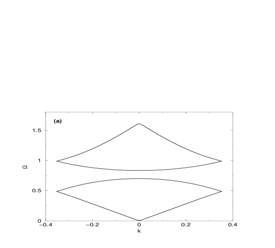
FIG. 5.: The dispersion curves for the almost sinusoidal configuration for different values of the control parameter $\lambda$. The curve (a) shows the situation when two branches are separated ($\lambda<0.05$). By increasing $\lambda$ they begin to overlap for $\lambda\approx 0.05$ (b), until $\lambda$ reaches the critical value $\lambda=0.25$. The curve (c) corresponds to $\lambda=0.249$. The finite slope of curves at $k=0$ coincides with that of the Goldstone mode. For $\lambda>0.25$ (d), these two brances combine into a single mode.

FIG. 6.: The dependence of the phase velocity of Goldstone mode on $\lambda$, corresponding to the almost sinusoidal configuration $s^{2}$.

FIG. 7.: Four lowest branches of collective modes for the simplest of non-sinusoidal state $sd$ for $\lambda=-1$. The branches for all other non-sinusoidal configurations are qualitatively same as that for $sd$.

FIG. 8.: The dependence of the phase velocity of Goldstone modes on the parameter $\lambda$ for all metastable non-sinusoidal configurations.

REFERENCES

- [1] P. A. Lee, T. M. Rice and P. W. Anderson, Solid State Commun. 14, 703 (1974).
- [2] G. Grüner, Rev. Mod. Phys. 60, 1129 (1988); G. Grüner, Density Waves in Solids (Addison-Wesley, 1994).
- [3] A. Bjeliš, in Applications of Statistical and Field Theory Methods to Condensed Matter, p. 325, eds. D. Baeriswyl et al (Plenum Press, 1990).
- [4] For reviews see Incommensurate Phases in Dielectrics, Vols. 1 and 2, eds. R. Blinc and A. P. Levanyuk (North-Holland, Amsterdam, 1986), and Ref. [5].
- [5] H. Z. Cummins, Phys. Rep. 185, 211 (1990).
- [6] W. L. McMillan, Phys. Rev. B 14, 1496 (1976); L. N. Bulaevski and D. I. Khomskii, Zh. Eksp. Teor. Fiz. 74, 1863 (1978) [Sov. Phys. JETP 47, 971 (1978)].
- [7] J. C. Tolédano and P. Tolédano, The Landau Theory of Phase Transitions (World Scientific, Singapore, 1987).
- [8] A. Bjeliš and M. Latković, Phys. Lett. A 198, 389 (1995).
- [9] M. Latković and A. Bjeliš, Phys. Rev. B 58, 11273 (1998).
- [10] P. Bak and J. von Boehm, Phys. Rev. B 21, 5297 (1980).
- [11] W. Selke, Phys. Rep. 170, 213 (1988).
- [12] S. Aubry, Phys. Rep. 103, 127 (1984).
- [13] J. L. Raimbault and S. Aubry, J. Phys.: Condens. Matter 7, 8287 (1995).
- [14] J. P. Lorenzo, Thèse, Université Paris VI (1998).
- [15] S. Aubry, in Soliton and Condensed Matter; Solid State Sci., Vol. 8, edited by A. R. Bishop and T. Schneider (Springer, 1978), p. 254.
- [16] S. Aubry and P. Quemerais, in Low-Dimensional Electronic Properties of Molybden Bronzes and Oxides, edited by C. Schlenker (Kluwer Academic Publishers, Dordrecht, 1989), p. 209.
- [17] C. Baesens and R. S. Mackay, J. Stat. Phys. 85, 471 (1996).
- [18] J. P. Lorenzo and S. Aubry, Physica D 113, 276 (1998).
- [19] V. Dananić, A. Bjeliš, M. Rogina and E. Coffou, Phys. Rev. A 46, 3551 (1992).
- [20] V. Dananić and A. Bjeliš, Phys. Rev. E 50, 3900 (1994).
- [21] R. M. Hornreich, M. Luban, and S. Shtrikman, Phys. Rev. Lett. 35, 1678 (1975).
- [22] A. Michelson, Phys. Rev. B 16, 577 (1977).
- [23] Y. Ishibashi and H. Shiba, J. Phys. Soc. Japan 45, 409 (1978).
- [24] A. D. Bruce, R. A. Cowley and A. F. Murray, J. Phys. C: Solid State Phys. 11, 3591 (1978).
- [25] A. P. Levanyuk and D. G. Sannikov, Fiz. Tverd. Tela 18, 1927 (1976) [Sov. Phys. Solid State 18, 1122 (1976)].
- [26] I. Aramburu, G. Madariaga and J. M. Pérez-Mato, Phys. Rev. B 49, 802 (1994).
- [27] H. Mashiyama, J. Korean Phys. Soc. (Proc. Suppl.) 27, S96 (1994).
- [28] D. G. Sannikov, Fiz. Tverd. Tela (St. Petersburg) 39, 1282 (1997) [Phys. Solid State 39, 1139 (1997)].
- [29] D. G. Sannikov and G. Schaack, J. Phys.: Condens. Matter 10, 1803 (1998).
- [30] M. Latković, V. Dananić and A. Bjeliš, to be published.
- [31] V. Dananić and A. Bjeliš, Phys. Rev. Lett. 80, 10 (1998).
- [32] A. D. Bruce and R. A. Cowley, Structural Phase Transitions (Taylor and Francis, London, 1981).
- [33] A. Aharony, E. Domany and R. M. Hornreich, Phys. Rev. B 36, 2006 (1987).
- [34] see, e.g., V. A. Yakhubovich and V. M. Starzhinskhii, Lyneinie differentsialnie uravnenia s periodicheskhimi koeffitsientami (Nauka, Moskva, 1972).
- [35] H. Poincaré, Acta Math. 13, 5 (1890).
- [36] M. Iwata, H. Orihara and Y. Ishibashi, J. Phys. Soc. Japan 67, 3130 (1998).
- [37] A. Bjeliš and S. Barišić, Phys. Rev. Lett. 48, 684 (1982); S. Barišić and A. Bjeliš, in Theoretical Aspects of Band Structure and Electronic Properties of Pseudo-One-Dimensional Solids, edited by H. Kamimura (Riedel, Dordrecht, 1985), p. 49.
- [38] K. Kawasaki, J. Phys. C: Solid State Phys. 16, 6911 (1983).
- [39] V. Dananić, A. Bjeliš and M. Latković, Fizika A (Zagreb) 8 383 (1999); http://arXiv.org/abs/cond-mat/0005257.