Finite Temperature Collapse of a Bose Gas with Attractive Interactions

Abstract

We study the mechanical stability of the weakly interacting Bose gas with attractive interactions, and construct a unified picture of the collapse valid from the low temperature condensed regime to the high temperature classical regime. As we show, the non-condensed particles play a crucial role in determining the region of stability, even providing a mechanism for collapse in the non-condensed cloud. Furthermore, we demonstrate that the mechanical instability prevents BCS-type “pairing” in the attractive Bose gas. We extend our results to describe domain formation in spinor condensates.

I introduction

The trapped Bose gas with attractive interactions is a novel physical system. At high densities such clouds are mechanically unstable; however at low densities they can be stabilized by quantum mechanical and entropic effects. Stability and collapse has been observed in clouds of degenerate ⁷Li [3] and ⁸⁵Rb [4]. The collapse of the Bose gas shares many features of the gravitational collapse of cold interstellar hydrogen, described by the Jeans instability [5]; related instabilities occur in supercooled vapors. Theoretical studies of the attractive Bose gas, typically numerical, have been limited to zero [6] or very low temperature [7, 8]. Here we give a simple analytic description of the region of stability and threshold for collapse valid from zero temperature to well above the Bose condensation transition, and thus provide a consistent global picture of the instability. As we see, at finite temperature, the phase diagram of the Bose gas includes regions where the non-condensed particles play a significant role in the collapse [9].

Our results are summarized in the phase diagram in Fig. 1 which shows three regions: normal, Bose condensed, and collapsed. This third region is not readily accessible experimentally; the system becomes unstable at the boundary (the solid line in the figure). In this figure the condensation and collapse lines actually meet at a finite angle. The gross features of the phase diagram can be understood qualitatively with dimensional arguments. At low temperatures the only stabilizing force is the zero-point motion of the atoms. This “quantum pressure” has a characteristic energy per particle of $E_{Q}\sim\hbar^{2}V^{-2/3}/m$, where $\hbar$ is Planck’s constant, $V$ is the volume in which the cloud is confined, and $m$ is the mass of an atom. The attractive interactions which drive the collapse are associated with an energy $U=\hbar^{2}a_{s}n/m$, where $n$ is the density, and $a_{s}$ ($=-1.45\,$nm for ⁷Li and $-20\,$nm for ⁸⁵Rb) is the s-wave scattering length. Comparison of $U$ with $E_{Q}$ suggests that for low temperatures the density $n$ at collapse should be $\sim(V^{2/3}a_{s})^{-1}$, independent of temperature. At high temperatures, the stabilizing force is thermal pressure, $P=-T\partial S/\partial V$, which is characterized by the thermal energy $E_{T}\sim k_{B}T$. Here comparison of $U$ with $E_{T}$ suggests that at high temperatures the density of collapse should be $\sim mk_{B}T/\hbar^{2}a_{s}$, linear in temperature. The crossover between the quantum and classical behaviors ($n\propto T^{0}$ and $n\propto T$) occurs near $T_{c}$. The collapse, as described here, is a phenomena in which the cloud as a whole participates, not just the condensate.

Our basic approach is to identify the collapse with an instability in the lowest energy mode of the system (the breathing mode in a spherically symmetric cloud). As the system goes from stable to unstable, the frequency of this mode goes from real to complex, passing through zero when the instability sets in. The density response function, $\chi(k,\omega)$, which measures the response of the cloud to a probe at wave vector $k$ and frequency $\omega$, diverges at the resonant frequencies of the cloud. Therefore, by virtue of the vanishing frequency of the lowest energy mode, the collapse is characterized by

$$\chi(k=2\pi/L,\omega=0)^{-1}=0.$$ (1)

Here $k=2\pi/L$ is the wave-vector of the unstable mode, whose wavelength $L$ should be of order the size of the system. Equation (1) implicitly determines the line of collapse in the temperature-density plane.

To evaluate the response function analytically, we use a local-density approximation, replacing the response function $\chi(k,\omega)$ of the inhomogeneous cloud by that of a gas with uniform density $n$. The response of the uniform gas is evaluated at the same frequency and wave-vector as for the inhomogeneous system, and $n$ is given by the central density of the atomic cloud. The local-density approximation should be valid for temperatures large enough that the thermal wavelength, $\Lambda_{T}=(2\pi\hbar^{2}/mk_{B}T)^{1/2}$, is much smaller than the size of the trap. In all experiments to date, this condition is satisfied, and we treat $k\Lambda_{T}$ as a small parameter in our calculation. With this approximation, we calculate the line of collapse using the well developed theory of $\chi(k,\omega)$ of a uniform gas (reviewed in [10]).

In the experiments on ⁷Li, the atoms are held in a magnetic trap with a harmonic confining potential $V(r)=\frac{1}{2}m\omega^{2}r^{2}$, with $\omega\approx 2\pi\times 145s^{-1}$[11]. This potential gives the cloud a roughly Gaussian density profile (see Sec. IV). The temperature $T$ is typically 50 times the trap energy $\hbar\omega\approx 7$nK, so the parameter $k\Lambda_{T}$, $\approx\sqrt{\hbar\omega/k_{B}T}\approx 0.14$, is small. The experiments on ⁸⁵Rb use softer traps, $\hbar\omega\approx 0.6$nK, and colder temperatures $T\approx 15$nK, so that $k\Lambda_{T}\approx 0.2$.

The goal of our approach is to provide a framework for investigating the interplay of condensation and collapse. Although our results are not as accurate as can be obtained numerically (comparing with previous numerical work [7], we find that are results are always well within a factor of two of those calculated using more sophisticated models), the conceptual and computational advantages of working with a uniform geometry far outway any loss in accuracy. Due to their simplicity, the arguments used here provide an essential tool to choosing which parameter ranges to investigate in future experiments and computations.

The tools introduced to discuss the collapse of an attractive gas can also be used to describe other instabilities in trapped Bose gases. In Section V and VI, we apply these methods to the problem of BCS type pairing between bosons, and towards domain formation in spinor condensates.

II Simple Limits

A Zero Temperature

To illustrate our approach we first consider the stability of a zero temperature Bose condensate. The excitation spectrum of a uniform gas is [12]:

$$\omega^{2}=\left(\frac{k^{2}}{2m}\right)^{2}+gn\frac{k^{2}}{m}\equiv E_{k}^{2},$$ (2)

where $g=4\pi\hbar^{2}a_{s}/m$. In the attractive case, $g<0$, all long wavelength modes with $k^{2}/2m<2|g|n$ have imaginary frequencies and are unstable. A system of finite size $L$ only has modes with $k>2\pi/L$, and for larger $k$ has an excitation spectrum similar to Eq. (2). If $|g|n<\hbar^{2}\pi^{2}/mL^{2}$, the unstable modes are inaccessible and the attractive Bose gas is stable.

This information is included in the density response function $\chi(k,\omega)$ of the dilute zero-temperature gas [10],

$$\chi(k,\omega)=\frac{2n\varepsilon_{k}}{\omega^{2}-E_{k}^{2}},$$ (3)

where $\varepsilon_{k}=k^{2}/2m.$ The poles of $\chi$ are at the excitation energies, $\pm E_{k}$. In particular, $\chi(k=2\pi/L,\omega=0)$ diverges when $|g|n=\hbar^{2}\pi^{2}/mL^{2}$.

B High Temperature ($T\gg T_{c}$)

We further illustrate our procedure by calculating the stability of an attractive Bose gas at temperature much larger than $T_{c}$, where thermal pressure is the predominant stabilizing force. Quantum effects are negligible in this limit, and the line of collapse is simply the spinodal line of the classical liquid-gas phase transition [13], as characterized by Mermin [14]. We neglect finite size effects, and look for an instability in the uniform gas at zero wavevector, $k=0$, corresponding to finding where $\chi(k=0,\omega=0)$ diverges. The susceptibility $\chi(0,0)=-\partial n/\partial\mu$ (where $\mu$ is the chemical potential), is proportional to the compressability of the system, which diverges when the gas becomes unstable.

At high temperature we work in the Hartree-Fock approximation, where the density is given by the self-consistent solution of

$$n=\int\frac{d^{3}p}{(2\pi\hbar)^{3}}\frac{1}{e^{\beta(\epsilon_{p}-\mu)}-1},$$ (4)

with Hartree-Fock quasiparticle energies $\epsilon_{p}=\varepsilon_{p}+2gn$; here $\beta=1/k_{B}T$. In the classical limit ($\beta\mu\ll-1$), $n=e^{\beta(\mu-2gn)}/\Lambda_{T}^{3}$. The response $\chi(0,0)$ has the structure of the random phase approximation (RPA),

$$\chi(k,\omega)=\frac{\chi_{0}(k,\omega)}{1-2g\chi_{0}(k,\omega)},$$ (5)

where $\chi_{0}(0,0)=-\left(\partial n/\partial\mu\right)_{\epsilon}$ (where the $\epsilon$ are held fixed) is the “bare” response. In the classical limit $\chi_{0}(0,0)=-\beta n$. Since $\chi_{0}(0,0)$ is negative, the repulsive system ($g>0$) is stable. However, for attractive interactions $g<0$), the denominator of Eq. (5) vanishes when $2g\chi_{0}=1$, which in the classical limit occurs when $2|g|n=k_{B}T$.

The above calculation is only valid well above $T_{c}$. When $|\mu|\sim\hbar^{2}/mL^{2}$, finite size effects start to become important, and a more sophisticated approach is needed. If one blindly used the above result near $T_{c}$ one would erroneously find that the instability towards collapse prevents Bose condensation from occurring. This difficulty can be avoided by working with the finite wave-vector response $\chi(k=2\pi/L,\omega=0)$, to which we now turn.

III Density Response Function

The approximation we shall use for $\chi$ is to treat the response of the gas in the RPA, with the simplifying assumption that the bare response of the condensed and non-condensed particles is taken to be the response of a non-interacting system. This approach, employed by Szépfalusy and Kondor [15] in studying the critical behavior of collective modes of a Bose gas, and later modified by Minguzzi and Tosi [16] to include exchange, is simple to evaluate analytically, and is valid both above and below $T_{c}$. It generates an excitation spectrum which is conserving [17] and gapless [10]. At zero temperature it yields the Bogoliubov spectrum, Eq. (2), and above $T_{c}$ it becomes the standard RPA with exchange.

The susceptibility in this approximation has the form,

$$\chi(k,\omega)=\frac{\chi_{0}^{c}+\chi_{0}^{n}+g\chi_{0}^{c}\chi_{0}^{n}}{(1-g\chi_{0}^{c})(1-2g\chi_{0}^{n})-4g^{2}\chi_{0}^{c}\chi_{0}^{n}},$$ (6)

where $\chi_{0}^{c}$ and $\chi_{0}^{n}$ are the condensate and non-condensed particle contributions to the response of the non-interacting cloud,

$$\chi_{0}^{n}(k,\omega) = \int\frac{d^{3}q}{(2\pi)^{3}}\frac{f(q-k/2)-f(q+k/2)}{\omega-(\varepsilon_{q+k/2}-\varepsilon_{q-k/2})},$$ (8)

$$\chi_{0}^{c}(k,\omega) = \frac{n_{0}}{\omega-\varepsilon_{k}}-\frac{n_{0}}{\omega+\varepsilon_{k}}.$$ (9)

Here $n_{0}$ is the condensate density, the $\varepsilon_{k}=k^{2}/2m$ are the free particle kinetic energies as before, and the Bose factors $f(k)$ are given by $(e^{-\beta(\varepsilon_{k}-\mu)}-1)^{-1}$. In Appendix A we briefly review the derivation of this response function. At zero temperature $\chi_{0}^{n}=0$ and the susceptibility reduces Eq. (3), while above $T_{c}$, $\chi_{0}^{c}=0$, and $\chi$ reduces to Eq. (5). Figure 2 shows the class of diagrams summed in this approximation.

Expanding $\chi_{0}^{n}$ in the small parameter $k\Lambda_{T}$ (see details in Appendix B), we derive for $T>T_{c}$,

$$g\chi_{0}^{n}(k,0)=-2\frac{a_{s}}{\Lambda_{T}}\left[\frac{4\pi}{k\Lambda_{T}}\arctan\left|{\epsilon_{k}}/{4\mu}\right|^{1/2}+g_{1/2}(e^{\beta\mu})-\left|{\pi}/{\beta\mu}\right|^{1/2}+{\cal O}(k\Lambda_{T})\right],$$ (10)

where $g_{\nu}(z)\equiv\sum_{j}z^{j}/j^{\nu}$ is the polylogarithm function. For chemical potential $\mu$ much larger in magnitude than $k_{B}T$, the system is classical, and Eq. (10) reduces to $g\chi_{0}^{n}=-\beta gn$, as in the Hartree-Fock approach, Sec. II B. Below $T_{c}$ the chemical potential of the non-interacting system vanishes and the response functions are:

$$g\chi_{0}^{n}(k,0) = -\frac{4\pi^{2}a_{s}}{k\Lambda_{T}^{2}}+{\cal O}((k\Lambda_{T})^{0}),$$ (12)

$$g\chi_{0}^{c}(k,0) = -16\pi\frac{a_{s}n_{0}}{k^{2}}.$$ (13)

Using these expressions we calculate the spinodal line separating the stable and unstable regions of Fig. 1 by setting $k=2\pi/L$ and solving the equation

$$\chi^{-1}\propto 1-g(\chi_{0}^{c}+2\chi_{0}^{n})-2g^{2}\chi_{0}^{c}\chi_{0}^{n}=0,$$ (14)

which gives the line of collapse as a function of $\mu$ and $T$ (for $T>T_{c}$) or as a function of $n_{0}$ and $T$ (for $T<T_{c}$). We use the following relations to plot the instability on the $n-T$ phase diagram,

$$n=\left\{\begin{array}[]{ll}\Lambda_{T}^{-3}g_{3/2}(e^{\beta\mu}),&\quad T>T_{c}\\ n_{0}+\Lambda_{T}^{-3}\zeta(3/2),&\quad T<T_{c}.\end{array}\right.$$ (15)

Equations (12) and (13) indicate that below $T_{c}$ the noncondensate response $\chi_{0}^{n}$ scales as $k^{-1}\sim L$, while the condensate response $\chi_{0}^{c}$ scales as $k^{-2}\sim L^{2}$. For realistic parameters, $L$ is the largest length in the problem, so that the condensate dominates the instability except when $n_{0}$ is much smaller than $n$. Since the condensate is very localized, even a few particles in the lowest mode make $n_{0}$ locally much greater than the density of noncondensed particles. In Fig. 3 we show how the line of instability depends on the size of the system, $L$.

From the above equations we calculate the maximum stable value of the condensate density $n_{0}$. The line of collapse crosses the line of condensation at a temperature $T^{*}=\hbar^{2}/2mk_{B}L|a|$. Above this temperature no condensation can occur. For $T<T^{*}$ the collapse limits the density of condensed particles to

$$(n_{0})_{\rm max}=\frac{\pi}{4L^{3}}\left(\frac{L}{|a|}\right)\left(\frac{T^{*}-T}{T^{*}+T}\right);$$ (16)

$(n_{0})_{\rm max}$ decreases monotonically with temperature, from the value $(n_{0})_{\rm max}^{\rm T=0}=\pi/4L^{2}|a|$, eventually vanishing at $T=T^{*}$. Using parameters from experiments [3, 4], we find for the Rice ⁷Li trap, $(N_{0})_{\rm max}^{\rm T=0}=L^{3}(n_{0})_{\rm max}^{\rm T=0}=1700$, and $T^{*}$ = 7.5 $\mu$K, while for the JILA ⁸⁵Rb trap, $(N_{0})_{\rm max}^{\rm T=0}=120$, and $T^{*}$ = 46 nK, The maximum number of particles vs. temperature for the two experiments are plotted in Fig. 4; these results are consistent with the experiments, and agree quite well with numerical mean-field calculations [7]. In particular, our curve $(N_{0})_{\rm max}(T)$ for lithium has a slope of $-1/2.2$ nK at $T=0$, which lies between the calculated slopes of Davis et al. and Houbiers et al. [7]. Although $(n_{0})_{\rm max}$ decreases with temperature, the non-condensed density $n^{\prime}$ increases ($n^{\prime}=\Lambda^{-3}\zeta(3/2)$). Thus the total density at collapse need not be monotonic with temperature (cf. the low temperature region of Fig. 1b).

Future condensate experiments at higher temperatures and densities should be able to study the structure in Eq. (16), and map out the phase diagram in Fig. 1. The rubidium experiments are performed at temperatures near $T^{*}$, where the spinodal line intersects $T_{c}$, and in principle should be able to explore the crossover between the quantum mechanical and classical behavior of the instability. The lithium experiments are much further away from exploring this regime, and in the current geometry, inelastic processes make such an investigation impractical [18]. Since $T^{*}$ is proportional to $1/L$, a softer trap could be used to bring this crossover down to lower temperatures where these difficulties are less severe (see Fig. 3). More precise numerical studies at higher temperatures are needed to guide these experiments.

IV Modeling the harmonic trap

Most experimental and theoretical results are reported in terms of numbers of particles instead of density. By appropriately modeling the density distribution of a harmonically trapped gas, we can present our conclusions in such a form. Once the interactions are strong enough to modify the density distribution significantly, the system undergoes collapse; thus we can take the density distribution to be that of non-interacting particles. For $k_{B}T\gg\hbar\omega$, the density profile is well-approximated by

$$n(r)=\int\!\!\frac{d^{3}p}{(2\pi)^{3}}\frac{1}{e^{\beta(\varepsilon_{p}+V(r)-\mu)}-1}+n_{0}e^{-r^{2}/d^{2}},$$ (17)

where $V(r)=m\omega^{2}r^{2}/2$ is the confining potential, with characteristic length $d=(\hbar/m\omega)^{1/2}$. The density of condensed particles at the center of the trap is $n_{0}$. Above $T_{c}$, $n_{0}=0$, and below $T_{c}$, $\mu=0$. Integrating over space, we have

$$N=\left\{\begin{array}[]{ll}\left({k_{B}T}/{\hbar\omega}\right)^{3}g_{3}(e^{\beta\mu}),&\quad T>T_{c}\\ \left({k_{B}T}/{\hbar\omega}\right)^{3}\zeta(3)+\left(\pi\hbar/m\omega\right)^{3/2}n_{0},&\quad T<T_{c}.\end{array}\right.$$ (18)

The instability occurs in the lowest energy mode of the system, the breathing mode, whose wave-vector is proportional to $1/d$. In a zero temperature non-interacting gas the breathing mode has a density profile $\delta\rho\propto(2r^{2}/d^{2}-3)\exp{(-r^{2}/d^{2})}$, where $r$ is the radial coordinate. In momentum space this distribution is peaked at wave-vector $k=2/d$. At finite temperature thermal pressure increases the radius of the cloud and the wave vector of the breathing mode becomes smaller. Since the response of the non-condensed cloud is relatively insensitive to the wave-vector, we look for an instability at $k=2/d$.

The resulting phase diagram, Fig. 5, is similar to that in Fig. 1. The most significant difference is that the line of collapse follows the condensation line (on the scale of the figure they appear to coincide over a significant temperature range). This behavior can be understood by noting that for trapped particles, condensation results in a huge increase in the central density of the cloud (a standard diagnostic of BEC).

V Pairing

With minor changes the formalism presented here can be used to investigate the instability towards forming loosely bound dimers, or “pairs,” the Evans-Rashid transition. Such an instability occurs in an electron gas at the superconducting BCS transition [20], and has been predicted by Houbiers and Stoof [7, 21] to occur in the trapped alkalis. The pairing is signalled by an instability in the T-matrix of the normal phase [22], which plays the role that the density response function plays in the collapse. Again, we simulate the finite size of the cloud by looking for an instability at $k=2\pi/L$, as opposed to $k=0$ in a bulk sample. In analogy to Eq. (5), the T-matrix can be written as a ladder sum,

$${\cal T}(k,\omega)=\frac{g}{1-g\Xi(k,\omega)}.$$ (19)

In this equation, $k$ is the relative momentum of the pair. The instability towards pairing is signalled by ${\cal T}\to\infty$, when $g\Xi=1$. To the same level of approximation as Eq. (8), the medium-dependent part of the “pair bubble” $\Xi$ is

$$\Xi(k,\omega)=\int\frac{d^{3}q}{(2\pi)^{3}}\frac{f(q-k/2)+f(q+k/2)}{\omega-(\varepsilon_{q+k/2}+\varepsilon_{q-k/2})}.$$ (20)

Setting $\omega=0$, and expanding in small $k\lambda_{T}$, we find

$$g\Xi(k,\omega=0)=-4\frac{a_{s}}{\Lambda_{T}}\left[\frac{4\pi}{k\Lambda_{T}}\arctan\left(\frac{\left|{\epsilon_{k}}/{4\mu}\right|^{1/2}}{1+\left|{\epsilon_{k}}/{4\mu}\right|^{1/2}}\right)+g_{1/2}(e^{\beta\mu})-\left|{\pi}/{\beta\mu}\right|^{1/2}+{\cal O}(k\Lambda_{T})\right].$$ (21)

Except for the argument of the arctangent, this expression is identical to twice $g\chi_{0}^{n}$ as given in Eq. (10). Since arctangent is a monotonic function, and its argument here is smaller than in Eq. (10), we see that $g\Xi<2g\chi_{0}^{n}$, which implies that the instability towards collapse occurs at a lower density than the pairing instability. Thus we conclude that the pairing transition does not occur in an attractive Bose gas. Interestingly, in the classical limit, the instabilities towards pairing and collapse coincide.

VI Domain Formation in Spinor Condensates

The approach used here to discuss the collapse of a gas with attractive interactions also describes domain formation in spinor condensates, and gives a qualitative understanding of experiments at MIT [23] in which optically trapped ²³Na is placed in a superposition of two spin states. Although all interactions in this system are repulsive, the two different spin states repel each other more strongly than they repel themselves, resulting in an effective attractive interaction. The collapse discussed earlier becomes, in this case, an instability towards phase separation and domain formation. The equilibrium domain structure is described in [24]. Here we focus on the formation of metastable domains.

The ground state of sodium has hyperfine spin $F=1$. In the experiments the system is prepared so that only the states $|1\rangle=|F=1,m_{F}=1\rangle$ and $|0\rangle=|F=1,m_{F}=0\rangle$ enter the dynamics. The effective Hamiltonian is then

$$H=\int\!\!d^{3}r\,\frac{\nabla\psi_{i}^{\dagger}\cdot\nabla\psi_{i}}{2m}+V(r)\psi_{i}^{\dagger}\psi_{i}+\frac{g_{ij}}{2}\psi^{\dagger}_{i}\psi^{\dagger}_{j}\psi_{j}\psi_{i}.$$ (22)

where $\psi_{i}$ ($i=0,1$) is the particle destruction operator for the state $|i\rangle$; summation over repeated indices is assumed. The effective interactions, $g_{ij}=4\pi\hbar^{2}a_{ij}/m$, are related to the scattering amplitudes $a_{F=0}$ and $a_{F=2}$, corresponding to scattering in the singlet ($F_{1}+F_{2}=0$) and quintuplet ($F_{1}+F_{2}=2$) channel, by [23, 24, 25]:

$$\tilde{a}\equiv a_{11}=a_{01}=a_{10}=a_{F=2},$$ (24)

$$\delta a\equiv a_{11}-a_{00}=(a_{F=2}-a_{F=0})/3.$$ (25)

Numerically, $\tilde{a}=2.75$nm and $\delta a=0.19$nm. We introduce $\tilde{g}=4\pi\hbar^{2}\tilde{a}/m$ and $\delta g=4\pi\hbar^{2}\delta a/m$. In the mean field approximation, the interaction in Eq. (22) becomes a function of $n_{m=0}$ and n, the density of particles in the state $|0\rangle$ and the total density, respectively:

$$\langle H_{int}\rangle=\int\!\!d^{3}r\,\left(\frac{\tilde{g}}{2}n^{2}-\frac{\delta g}{2}n_{m=0}^{2}\right),$$ (26)

which shows explicitly the effective attractive interaction. Initially the condensate is static with density $n=10^{14}{\rm cm}^{-3}$, and all particles in state $|1\rangle$. A radio-frequency pulse places half the atoms in the $|0\rangle$ state without changing the density profile. Subsequently the two states phase separate and form domains from 10 to 50 $\mu$m thick. The trap plays no role here, so we can neglect $V(r)$ in Eq. (22) and consider a uniform cloud.

Linearizing the equations of motion with an equal density of particles in each state, we find two branches of excitations corresponding to density and spin waves [26],

$$\omega_{ph}^{2} = \left(\frac{k^{2}}{2m}\right)^{2}+\tilde{g}n\frac{k^{2}}{m}+{\cal O}(\delta g),$$ (28)

$$\omega_{sp}^{2} = \left(\frac{k^{2}}{2m}\right)^{2}-\delta g\,n\frac{k^{2}}{4m}+{\cal O}((\delta g)^{2}).$$ (29)

Since $\delta g>0$ spin excitations with imaginary frequencies appear. The mode with the largest imaginary frequency grows most rapidly, and the width of the domains formed should be comparable to the wavelength $\lambda$ of this mode. By minimizing Eq. (29) we find $\lambda=\sqrt{2\pi/n\,\delta a}=10\mu$m, in rough agreement with the observed domain size.

VII Acknowledgements

The authors are grateful to the Ecole Normale Supérieure in Paris, and the Aspen Center for Physics, where this work was carried out. We owe special thanks to Eugene Zaremba and Dan Sheehy for critical comments. We are particularly indebted to Henk Stoof for his insightful recommendations and stimulating discussions, including raising the question of the relation between the instabilities towards pairing and collapse. This research was supported in part by the Canadian Natural Sciences and Engineering Research Council, and National Science Foundation Grant No. PHY98-00978, and facilitated by the Cooperative Agreement between the University of Illinois at Urbana-Champaign and the Centre National de la Recherche Scientifique.

A Review of the RPA

Here we give a brief derivation of the response function $\chi(k,\omega)$, Eq. (6), used in this paper. Generically, the response of a gas, $\chi=\delta n/\delta U$, is the direct response to the perturbation $\chi_{0}$ plus the response to the mean field generated by the disturbed atoms. For a normal gas in the Hartree approximation, $\delta n=\chi_{0}\delta U+\chi_{0}g\delta n$, while including exchange gives $\delta n=\chi_{0}\delta U+\chi_{0}2g\delta n$, as in Eq. (5). The RPA amounts to making a simple particular approximation to the polarization part $\chi_{0}$. For our purposes it suffices to take $\chi_{0}=\chi_{0}^{n}$, the response of an ideal gas, Eq. (8).

Generalizing the Hartree approximation to the condensed gas simply requires replacing $\chi_{0}$ with the response of the non-condensed particles $\chi_{0}^{n}$ plus the response of the condensate $\chi_{0}^{c}$, Eq. (9).

Including exchange in the degenerate gas requires some work, since exchange only occurs in interactions involving non-condensed atoms. A simple technique, demonstrated by Minguzzi and Tosi [16] is to look separately at the change in the density of condensed and non-condensed atoms, $\delta n_{0}$ and $\delta\tilde{n}$. Within Hartree-Fock these changes are related to the applied perturbation $\delta U$ by

$$\left(\begin{array}[]{c}\delta n_{0}\\ \delta\tilde{n}\end{array}\right)=\left(\begin{array}[]{c}\chi_{0}^{c}\\ \chi_{0}^{n}\end{array}\right)\delta U+\left(\begin{array}[]{cc}\chi_{0}^{c}&2\chi_{0}^{c}\\ 2\chi_{0}^{r}&2\chi_{0}^{r}\end{array}\right)\left(\begin{array}[]{c}g\delta n_{0}\\ g\delta\tilde{n}\end{array}\right),$$ (A1)

which gives the relationship

$$\chi=\frac{\delta n_{0}}{\delta U}+\frac{\delta\tilde{n}}{\delta U}=\frac{\chi_{0}^{c}+\chi_{0}^{n}+g\chi_{0}^{c}\chi_{0}^{n}}{(1-g\chi^{c}_{0})(1-2g\chi^{n}_{0})-4g^{2}\chi^{c}_{0}\chi^{n}_{0}}.$$ (A2)

Diagrammatic expressions for these different approximations are shown in Fig. 2.

B Asymptotic Expansions

In this Appendix we derive the $k\Lambda_{T}\to 0$ asymptotic expansions for the functions $\chi_{0}^{n}$ and $\Xi$, defined by Eqs. (8) and (20). These expansions are constructed to be valid for all $\mu$. We begin by breaking $\chi_{0}^{n}$ into two terms, one containing $f(q-k/2)$ and one containing $f(q+k/2)$. After shifting $q$ by $\pm k/2$ and integrating out the angular variables, we have

$$\chi_{0}^{n}(k,\omega)=\frac{m}{(2\pi)^{2}k}\int_{0}^{\infty}\!\!dq\,q^{2}\,f(q)\log\left[\frac{(\bar{p}+k/2-q)(\bar{p}-k/2+q)}{(\bar{p}+k/2+q)(\bar{p}-k/2-q)}\right],$$ (B1)

with $\bar{p}=m\omega/k$. We extract the important structure by rewriting the logarithm as an integral of the form $\int dx/x$. Scaling all lengths by a multiple of the thermal wavelength, we find

$$\chi_{0}^{n}(k,\omega) = \frac{-m}{\pi k\Lambda_{T}^{2}}\int_{z_{-}}^{z_{+}}\!\!dz\,I(z)$$ (B2)

$$I(z) = \int_{-\infty}^{\infty}\!\!dx\frac{x}{x-z}\frac{1}{e^{x^{2}-\beta\mu}-1},$$ (B3)

where $z_{\pm}=\omega/2\sqrt{\varepsilon_{k}T}\pm k\Lambda_{T}/4\sqrt{\pi}$. The integral $I(z)$ has been characterized by Szépfalusy and Kondor [15]. In particular, by expanding the distribution function in terms of Matsubara frequencies, one arrives at the $z\to 0$ asymptotic expansion,

$$I(z) = \sqrt{\pi}g_{1/2}(e^{\beta\mu})-\frac{i\pi z}{2}+i\pi\left(\frac{z}{z+i\sqrt{-\beta\mu}}\right)$$ (B5)

$$-2\pi\sum_{j=1}^{\infty}z^{j}\sum_{\nu=1}^{\infty}\Re\left[(-\beta\mu+2\pi i\nu)^{-(j+1)/2}\right],$$

where $\Re(z)$ is the real part of $z$. Integration of the leading terms gives Eq. (10).

Following a similar procedure of integrating out the angular variables we write $\Xi$ as

$$\Xi(k,\omega)=\frac{-2m}{\pi k\Lambda_{T}^{2}}\int_{\bar{z}_{-}}^{\bar{z}_{+}}\!\!dz\,I(z),$$ (B6)

with $\bar{z}_{\pm}=(k\Lambda/4\sqrt{\pi})[i\sqrt{1+2\omega/\varepsilon_{k}}\pm 1]$. Using the expansion in Eq. (B5) gives Eq. (21).

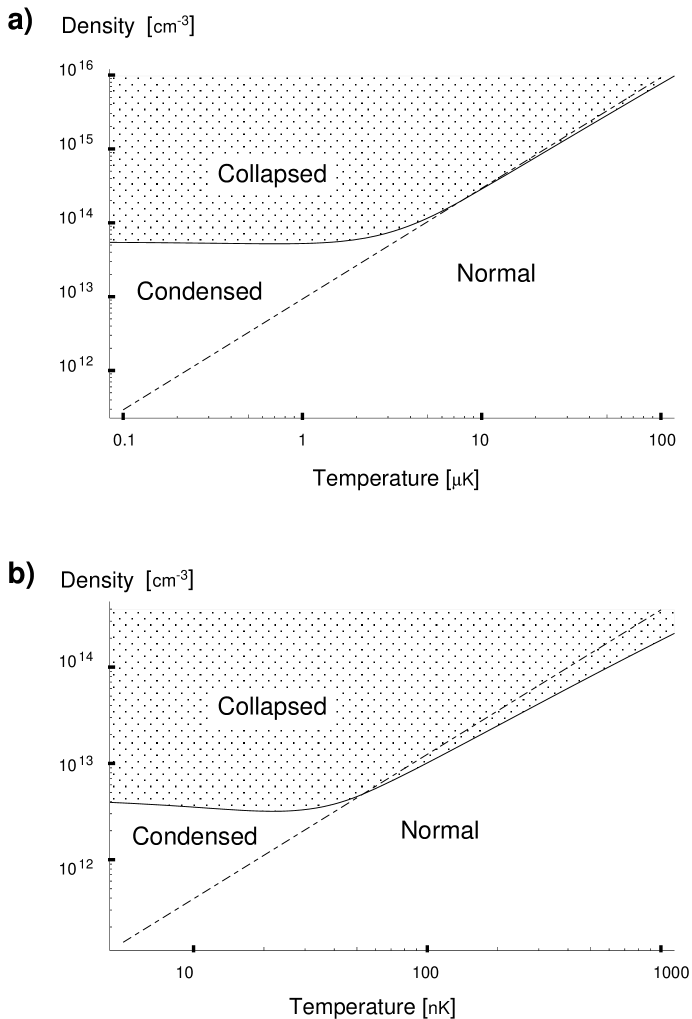
FIG. 1.: Phase diagram, density $n$ [cm^-3] versus temperature $T$, for a cloud of attractive bosons. a) For a cloud of ⁷Li with spatial extent $L=3.15\mu$m, scattering length $a_{s}=-1.45$nm, corresponding to the experiments in Ref. [1], performed at temperatures $T$ near $300$ nK. b) For a cloud of ⁸⁵Rb with scattering length $a_{s}=-20$nm and spatial extent $L=3\mu$m, corresponding to the recent experiments in Ref. [2], performed at $T$ near 15 nK.
Note the logarithmic scales. The solid line separates the unstable (shaded) region from the stable region. The dashed line, representing the Bose condensation transition has been continued into the collapsed region to illustrate that the two lines intersect. This diagram is drawn for a uniform but finite cloud, but can be applied to harmonically trapped gases by taking $n$ to be the central density in the trap.

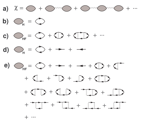
FIG. 2.: Diagrammatic description of the approximation used for the response function. Lines with arrows represent propagators of the non-interacting system. Jagged lines represent the contact interaction between particles. a) Generically the response function can be expressed in terms of a polarization bubble (the bubble with shaded interior). b) In the Hartree approximation (RPA), the polarization bubble is taken to be the response of the non-interacting gas. c) In the Hartree-Fock approximation, the polarization bubble involves a sum over repeated interactions. d) In a condensed system, the polarization bubble for the Hartree approximation must include terms where one of the particles is in the condensate. e) The Hartree-Fock approximation for the condensed gas requires writing all exchange graphs. This series is most easily summed by the matrix approach in Appendix A.

FIG. 3.: Scaling of the instability threshold with system size. Solid lines show the maximum stable density $n_{\rm max}$ for a given temperature. From the top, the system size is $L$ = 0.3, 3, 30 $\mu$m. The other parameters are the same as in Fig. 1a). The dashed line indicates the Bose-Einstein condensation transition. Note the three scaling regimes; at low temperature, $n_{\rm max}\sim L^{2}$, near the critical temperature $n_{\rm max}\sim L^{3/2}$, and at high temperatures $n_{\rm max}$ is independent of $L$ (see Eqs. (5) and (6)).

FIG. 4.: Maximum number of condensed particles as a function of temperature, for the a) ⁷Li and b) ⁸⁵Rb experiments. The $(k\Lambda_{T})^{0}$ terms in Eq. 12 have been included in producing these plots.

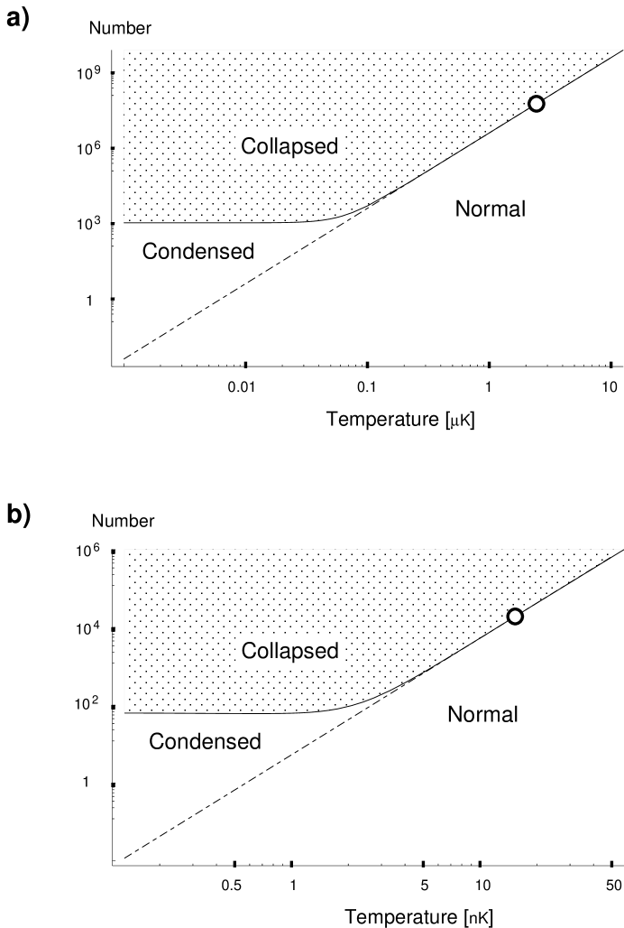
FIG. 5.: Phase diagram, number $N$ versus temperature $T$, for harmonically trapped bosons with attractive interactions; a) ⁷Li, b) ⁸⁵Rb. The parameters used correspond to Fig. 1. The open circle marks where the spinodal line meets with the BEC phase transition.

REFERENCES

- [1] Electronic address: emuelle1@uiuc.edu
- [2] Electronic address: gbaym@uiuc.edu
- [3] C.A. Sackett, H.T.C. Stoof, and R.G. Hulet, Phys. Rev. Lett. 80 2031, (1998); C.A. Sackett, C.C. Bradley, M. Welling, and R.G. Hulet, Appl. Phys. B 65 433, (1997); C.C. Bradley, C.A. Sackett, and R.G. Hulet, Phys. Rev. Lett. 78 985, (1997); C.C. Bradley, C.A. Sackett, and R.G. Hulet, Phys. Rev. A 55 3951, (1997).
- [4] S. L. Cornish, N. R. Claussen, J. L. Roberts, E. A. Cornell, and C. E. Wieman, preprint, cond-mat/0004290.
- [5] For elementary discussions of the Jeans instability see, e.g., R. Bowers, and T. Deeming Astrophysics II; Interstellar Matter and Galaxies (Jones and Bartlett, Sudbury, MA, 1984).
- [6] P.A. Ruprecht, M.J. Holland, K. Burnett, and M. Edwards, Phys.Rev. A 51, 4704 (1995); G. Baym and C. J. Pethick, Phys. Rev. Lett. 76, 6 (1996).
- [7] M.J. Davis, D.A.W. Hutchinson, and E. Zaremba, J. Phys. B 32, 3993 (1999); T. Bergeman, Phys. Rev. A 55, 3658 (1997); M. Houbiers and H.T.C. Stoof, Phys. Rev. A 54, 5055 (1996); P.A. Ruprecht, M.J. Holland, K. Burnett, and M. Edwards, Phys. Rev. A 51, 4704 (1995).
- [8] The very recent variational calculation of J. Tempere, F. Brosens, L. F. Lemmens and J. T. Devreese, Phys. Rev. A, 61, 043605 (2000), is capable of describing the complete phase diagram, and provides a complementary approach to the one studied here.
- [9] Previous theoretical studies [7] focused on the stability of the condensate at very low temperatures and in a regime where the density of non-condensed particles is much smaller than the condensate density. These studies found that the non-condensed particles play a very small role in the collapse. For example, Houbiers et al. concluded that the non-condensed particles are involved in the collapse only in so far as they change the geometry of the effective potential felt by the condensate. In this low temperature regime our results are consistent with these previous works.
- [10] A. Griffin, Excitations in a Bose-Condensed Liquid (Cambridge University Press, Cambridge, 1993).
- [11] The traps used are slightly asymmetric, and the frequencies quoted here are the geometric mean of the three frequencies along each principal axis; see [3, 4].
- [12] N.N. Bogoliubov, J. Phys. USSR, 11, 23 (1947).
- [13] In the theory of liquid-gas phase transitions, the spinodal line is the curve on the phase diagram where , which represents the edge of the co-existence region, beyond which supercooled vapor cannot exist.
- [14] N.D. Mermin, Ann. Phys. 18, 421, 454 (1962); 21, 99 (1963).
- [15] P. Szépfalusy and I. Kondor, Ann. Phys. 82, 1 (1974).
- [16] A. Minguzzi and M. P. Tosi, J. Phys: Condens. Matter 9, 10211 (1997).
- [17] G. Baym, Phys. Rev. 127, l39l (1962).
- [18] At a temperature of K, a m cloud of 7Li collapses at a density of . At such a high density the dominant decay mechanism is three-body collisions, giving a lifetime . Using the theoretical estimate [19], , we find that . At K the lifetime is only .
- [19] A. J. Moerdijk, H. M. J. M. Boesten, and B. J. Verhaar, Phys. Rev. A 53, 916 (1996); C. A. Sackett, J. M. Gerton, M. Welling, and R. G. Hulet, Phys. Rev. Lett. 82, 876 (1999).
- [20] J. Bardeen, L. N. Cooper, and J. R. Schrieffer, Phys. Rev. 108, 1175 (1957).
- [21] H. T. C. Stoof, Phys. Rev. A 49, 3824 (1994).
- [22] L.P. Kadanoff and G. Baym, Quantum Statistical Mechanics (W.A. Benjamin, New York, 1962).
- [23] H.-J. Miesner, D. M. Stamper-Kurn, J. Stenger, S. Inouye, A. P. Chikkatur, and W. Ketterle, Phys. Rev. Lett. 82, 2228 (1999).
- [24] T. Isoshima, K. Machida, and T. Ohmi, Phys. Rev. A 60, 4857 (1999).
- [25] T.-L. Ho, Phys. Rev. Lett. 81, 742 (1998).
- [26] Similar excitation spectra are found in E.V. Goldstein and P. Meystre, Phys. Rev. A 55, 2935 (1997).