Dynamics of vortex tangle without mutual friction in superfluid ⁴He

Abstract

A recent experiment has shown that a tangle of quantized vortices in superfluid ⁴He decayed even at mK temperatures where the normal fluid was negligible and no mutual friction worked. Motivated by this experiment, this work studies numerically the dynamics of the vortex tangle without the mutual friction, thus showing that a self-similar cascade process, whereby large vortex loops break up to smaller ones, proceeds in the vortex tangle and is closely related with its free decay. This cascade process which may be covered with the mutual friction at higher temperatures is just the one at zero temperature Feynman proposed long ago. The full Biot-Savart calculation is made for dilute vortices, while the localized induction approximation is used for a dense tangle. The former finds the elementary scenario: the reconnection of the vortices excites vortex waves along them and makes them kinked, which could be suppressed if the mutual friction worked. The kinked parts reconnect with the vortex they belong to, dividing into small loops. The latter simulation under the localized induction approximation shows that such cascade process actually proceeds self-similarly in a dense tangle and continues to make small vortices. Considering that the vortices of the interatomic size no longer keep the picture of vortex, the cascade process leads to the decay of the vortex line density. The presence of the cascade process is supported also by investigating the classification of the reconnection type and the size distribution of vortices. The decay of the vortex line density is consistent with the solution of the Vinen’s equation which was originally derived on the basis of the idea of homogeneous turbulence with the cascade process. The cascade process revealed by this work is an intrinsic process in the superfluid system free from the normal fluid. The obtained result is compared with the recent Vinen’s theory which discusses the Kelvin wave cascade with sound radiation.

I INTRODUCTION

Superfluid ⁴He (Helium II) behaves like an irrotational ideal fluid, whose characteristic phenomena can be explained well by the Landau two-fluid model. However, superflow becomes dissipative (superfluid turbulence) above some critical velocity. The concept of superfluid turbulence was introduced by Feynman [1] who stated that the superfluid turbulent state consists of a disordered set of quantized vortices, [2, 3] called vortex tangle(VT). Reminding the inertial range of the classical-fluid turbulence, Feynman proposed that VT undergoes the following cascade process. At zero temperature, a large distorted vortex loop breaks up to smaller loops through reconnections, and the cascade process continues self-similarly down to the order of the interatomic scale. At finite temperatures, however, normal fluid collides with vortices and takes energy from them.

This idea was developed further by Vinen. In order to describe an amplification of a temperature difference at the ends of a capillary retaining thermal counterflow, Gorter and Mellink introduced some additional interactions between the normal fluid and superfluid. [4] Through experimental studies of the second-sound attenuation, Vinen considered this Gorter-Mellink mutual friction in relation to the macroscopic dynamics of the VT. [5] Assuming homogeneous superfluid turbulence, Vinen obtained an evolution equation for the vortex line density (VLD) $L(t)$, what we call the Vinen’s equation

$$\frac{dL}{dt}=\alpha|\mbox{\boldmath$v$}_{\rm ns}|L^{3/2}-\chi_{2}\frac{\kappa}{2\pi}L^{2},$$ (1)

where $\alpha$ and $\chi_{2}$ are parameters dependent on temperature and $\mbox{\boldmath$v$}_{\rm ns}$ is the relative velocity between the normal flow and superflow, $\kappa$ the quantized circulation. This Vinen’s theory could describe well a large number of observations of mostly stationary cases.

However the nonlinear and nonlocal dynamics of vortices had long delayed the progress in further microscopic understanding of the VT. It was Schwarz that broke through. [6, 7] His most important contribution was that the direct numerical simulation of vortex dynamics connected with the scaling analysis enabled us to calculate such physical quantities as the VLD, some anisotropic parameters, the mutual friction force, etc. The observable quantities obtained by Schwarz’s theory agree well with the experimental results of the steady state of the VT. This research field pioneered by Schwarz has revealed many problems of vortex dynamics, such as the flow properties in channels  [8, 9, 10, 11], sideband instability of Kelvin waves, [12] vortex array in rotating superfluid, [13] vortex pinning. [14, 15]

The mutual friction plays an important role in the above vortex dynamics. The stationary state of the VT Schwarz obtained is self-sustaining, and realized by the competition between the excitation and dissipation due to the mutual friction subject to the $\mbox{\boldmath$v$}_{\rm ns}$ field, as described in the next section. Hence the system free from the mutual friction cannot sustain the stationary VT.

Compared with the steady state, there have been less studies of the transient behavior of the VT. Although the transient behavior generally refers to both the growth and decay process, this paper considers only the decay of the VT after the driving velocity is suddenly reduced to zero. The early measurements by Vinen [5] and the later ones [16, 17] observed a decay of the VT which was consistent with the Vinen’s equation (1) with only the decay term, although Schwarz and Rozen [17] coupled the Vinen’s equation with the hydrodynamical equations of the normal flow and the superflow in order to explain a slow decay following an initial rapid decay they observed. Apart from these experiments on thermal counterflow, the decay of vorticity in turbulence generated by towing a grid was studied recently. [18, 19] This turbulence is expected to be homogeneous and isotropic. The experimental results may be understood by the picture that the mutual friction can be so strong that the normal fluid and the superfluid lock together, behaving effectively like a single fluid. [20, 21] The experimental results are compared with the change in the turbulent energy spectrum which includes the Kolmogorov law.

Both these numerical and experimental results are much affected by the mutual friction. However, recently, Davis et al. [22] observed that vortices did decay even at mK temperatures where the normal fluid density became vanishingly small and, as a consequence, the mutual friction did not work effectively. The vortices were created by a vibrating grid, and detected by their trapping of negative ions. The first important point is that the vortices actually decay at such low temperatures. The second is that the decay rate becomes independent of temperature below $T\simeq 70$mK. It is unclear how the vortices decay. This experimental work, which is just preliminary at present, can develop a new research field of superfluid or vortex dynamics at mK temperatures; it can reveal some essence that may be covered with the normal fluid at higher temperatures.

Motivated by this experimental work, we study numerically the vortex dynamics without the mutual friction. The calculation under the localized induction approximation(LIA) is made for the dense VT, while the full Biot-Savart calculation for the more dilute vortices. The absence of the mutual friction makes the vortices kinked, which promotes vortex reconnections. Consequently small vortices are cut off from a large one through the reconnections. The resulting vortices also follow the self-similar process to break up to smaller ones. Although our formulation cannot describe the final destiny of the minimum vortex, the decay of the VT is found to be connected with this cascade process, which is just the cascade process at zero temperature Feynman proposed. [1]

The contents of this paper are the following. Section II describes the equations of motion of vortices and the method of numerical calculation. Section III studies the dynamics of dilute vortices under the full Biot-Savart law both without and with solid boundaries; this calculation reveals the essence of the cascade process. The dynamics of the dense VT under the LIA is discussed in Sec. IV. The obtained results are compared with the solution of the Vinen’s equation in Sec. V. The agreement is good, which supports the picture of the cascade process. The decay of the VT subject to the mutual friction is discussed too. Section VI is devoted to conclusions and discussions.

II EQUATIONS OF MOTION AND NUMERICAL SIMULATION

A quantized vortex is represented by a filament passing through the fluid and has a definite direction corresponding to its vorticity. Except for the thin core region, the superflow velocity field has a classically well-defined meaning and can be described by ideal fluid dynamics. The velocity produced at a point $r$ by a filament is given by the Biot-Savart expression :

$$\mbox{\boldmath$v$}_{s,\omega}=\frac{\kappa}{4\pi}\int_{\cal L}\frac{(\mbox{\boldmath$s$}_{1}-\mbox{\boldmath$r$})\times d\mbox{\boldmath$s$}_{1}}{|\mbox{\boldmath$s$}_{1}-\mbox{\boldmath$r$}|^{3}},$$ (2)

where $\kappa$ is the quantized circulation. The filament is represented by the parametric form $\mbox{\boldmath$s$}=\mbox{\boldmath$s$}(\xi,t)$, $\mbox{\boldmath$s$}_{1}$ refers to a point on the filament and the integration is taken along the filament. The Helmholtz’s theorem for a perfect fluid states that the vortex moves with the superfluid velocity at the point. Attempting to calculate the velocity $\mbox{\boldmath$v$}_{s,\omega}$ at a point $\mbox{\boldmath$r$}=\mbox{\boldmath$s$}$ on the filament makes the integral diverge as $\mbox{\boldmath$s$}_{1}\rightarrow\mbox{\boldmath$s$}$. To avoid it, we divide the velocity $\dot{\mbox{\boldmath$s$}}$ of the filament at the point $s$ into two components [6]:

$$\dot{\mbox{\boldmath$s$}}=\frac{\kappa}{4\pi}\mbox{\boldmath$s$}^{\prime}\times\mbox{\boldmath$s$}^{\prime\prime}\ln\left(\frac{2(\ell_{+}\ell_{-})^{1/2}}{e^{1/4}a_{0}}\right)+\frac{\kappa}{4\pi}\int_{\cal L}^{{}^{\prime}}\frac{(\mbox{\boldmath$s$}_{1}-\mbox{\boldmath$r$})\times d\mbox{\boldmath$s$}_{1}}{|\mbox{\boldmath$s$}_{1}-\mbox{\boldmath$r$}|^{3}}.$$ (3)

The first term shows the localized induction field arising from a curved line element acting on itself, and $\ell_{+}$ and $\ell_{-}$ are the lengths of the two adjacent line elements that hold the point $s$ between, and the prime denotes differentiation with respect to the arc length $\xi$. The mutual perpendicular vectors $\mbox{\boldmath$s$}^{\prime}$, $\mbox{\boldmath$s$}^{\prime\prime}$ and $\mbox{\boldmath$s$}^{\prime}\times\mbox{\boldmath$s$}^{\prime\prime}$ point along the tangent, the principal normal and the binormal at the point $s$, respectively, and their magnitudes are 1, $R^{-1}$ and $R^{-1}$, where $R$ is the local radius of curvature. The parameter $a_{0}$ is a cutoff parameter corresponding to a core radius. Thus the first term tends to move the local point $s$ with a velocity inversely proportional to $R$, along the binormal direction. The second term represents the nonlocal field obtained by carrying out the integral of Eq. (2) along the rest of the filament. The approximation that describes the vortex dynamics neglecting the nonlocal terms and replacing Eq. (3) by

$$\dot{\mbox{\boldmath$s$}}=\beta\mbox{\boldmath$s$}^{\prime}\times\mbox{\boldmath$s$}^{\prime\prime}$$ (4)

is called the localized induction approximation(LIA). Here the coefficient $\beta$ is defined by

$$\beta=\frac{\kappa}{4\pi}\ln\left(\frac{c<R>}{a_{0}}\right),$$ (5)

where $c$ is a constant of order 1 and $(\ell_{+}\ell_{-})^{1/2}$ is replaced by the characteristic radius $<R>$.

When boundaries are present, the boundary-induced field $\mbox{\boldmath$v$}_{s,b}$ is added to $\mbox{\boldmath$v$}_{s,\omega}$ so that the boundary condition $(\mbox{\boldmath$v$}_{s,\omega}+\mbox{\boldmath$v$}_{s,b})\cdot\hat{\mbox{\boldmath$n$}}=0$ can be satisfied. If the boundaries are specular plane surfaces, $\mbox{\boldmath$v$}_{s,b}$ is just the field by an image vortex made by reflecting the vortex into the plane and reversing its direction of the vorticity. Some other applied field $\mbox{\boldmath$v$}_{s,a}$, if present, is added, which results in the total velocity $\dot{\mbox{\boldmath$s$}}_{0}$ of the vortex filament without dissipation:

$$\dot{\mbox{\boldmath$s$}}_{0}= \frac{\kappa}{4\pi}\mbox{\boldmath$s$}^{\prime}\times\mbox{\boldmath$s$}^{\prime\prime}\ln\left(\frac{2(\ell_{+}\ell_{-})^{1/2}}{e^{1/4}a_{0}}\right)$$ (6)

$$+ \frac{\kappa}{4\pi}\int_{\cal L}^{{}^{\prime}}\frac{(\mbox{\boldmath$s$}_{1}-\mbox{\boldmath$r$})\times d\mbox{\boldmath$s$}_{1}}{|\mbox{\boldmath$s$}_{1}-\mbox{\boldmath$r$}|^{3}}+\mbox{\boldmath$v$}_{s,b}(\mbox{\boldmath$s$})+\mbox{\boldmath$v$}_{s,a}(\mbox{\boldmath$s$}).$$ (7)

At finite temperatures the mutual friction due to the interaction between the vortex core and the normal fluid flow $\mbox{\boldmath$v$}_{n}$ is taken into account. Then the velocity of a point $s$ is given by [2]

$$\dot{\mbox{\boldmath$s$}}=\dot{\mbox{\boldmath$s$}}_{0}+\alpha\mbox{\boldmath$s$}^{\prime}\times(\mbox{\boldmath$v$}_{n}-\dot{\mbox{\boldmath$s$}}_{0})-\alpha^{\prime}\mbox{\boldmath$s$}^{\prime}\times[\mbox{\boldmath$s$}^{\prime}\times(\mbox{\boldmath$v$}_{n}-\dot{\mbox{\boldmath$s$}}_{0})],$$ (8)

where $\alpha$ and $\alpha^{\prime}$ are the temperature-dependent friction coefficients, and $\dot{\mbox{\boldmath$s$}}_{0}$ is calculated from Eq.(7). All calculations in this work are made for $\alpha^{\prime}=0$. [6]

As discussed by Barenghi and Samuels [20], this formulation is essentially kinematic in the sense that the driving flows $\mbox{\boldmath$v$}_{n}$ and $\mbox{\boldmath$v$}_{s,a}$ are constant, that is, they only act on the vortex dynamics but are never affected by it. When the dynamics of the driving flows is concerned, it should be coupled selfconsistently to the vortex dynamics. However, since this work studies the system without the normal fluid and the driving superflow, this formulation will be useful to describe correctly the vortex dynamics, except for the phenomena that is concerned with the vortex core region, such as vortex reconnection, nucleation and annihilation.

Studying the vortex dynamics without the mutual friction needs to understand qualitatively the role of the mutual friction. [6] Let us assume the LIA and neglect the term with $\alpha^{\prime}$. Then Eqs. (7) and (8) are reduced to

$$\dot{\mbox{\boldmath$s$}}=\beta\mbox{\boldmath$s$}^{\prime}\times\mbox{\boldmath$s$}^{\prime\prime}+\mbox{\boldmath$v$}_{s,a}+\alpha\mbox{\boldmath$s$}^{\prime}\times(\mbox{\boldmath$v$}_{n}-\mbox{\boldmath$v$}_{s,a}-\beta\mbox{\boldmath$s$}^{\prime}\times\mbox{\boldmath$s$}^{\prime\prime}).$$ (9)

If the mutual friction is absent, the dynamics due to only the self-induced velocity conserves the total line length of vortices. Under the above mutual friction, one can easily find that when the applied relative flow $\mbox{\boldmath$v$}_{n}-\mbox{\boldmath$v$}_{s,a}$ blows against the local self-induced velocity $\beta\mbox{\boldmath$s$}^{\prime}\times\mbox{\boldmath$s$}^{\prime\prime}$, the mutual friction always shrinks the vortex line locally. On the other hand, the relative flow along the self-induced velocity yields a critical radius of curvature

$$R_{c}\simeq\frac{\beta}{|\mbox{\boldmath$v$}_{n}-\mbox{\boldmath$v$}_{s,a}|}.$$ (10)

When the local radius $R$ at a point on a vortex is smaller than $R_{c}$, the vortex will shrink locally, while the vortex of $R>R_{c}$ balloons out. Thus it should be noted that the mutual friction plays the dual role of the growth and decay of vortex line length. This dual role of the mutual friction sustains the steady state of the VT subject to the applied flow, where the highly curved structure whose local radius of curvature is less than $R_{c}$ will be smoothed out. If this applied field is absent, $R_{c}$ becomes infinite so that an arbitrary curved configuration of vortex lines shrinks away.

Here we will describe shortly the dynamical scaling discussed by Swanson and Donnelly, [23] and Schwarz [7], which is necessary for understanding the cascade process of the VT dynamics. Using the LIA and absorbing the factor $\beta$ into reduced time $t_{0}=\beta t$ and velocity $\mbox{\boldmath$v$}_{0}=\mbox{\boldmath$v$}/\beta$, Eq. (8) becomes

$$\frac{\partial\mbox{\boldmath$s$}}{\partial t_{0}}= \mbox{\boldmath$s$}^{\prime}\times\mbox{\boldmath$s$}^{\prime\prime}+\mbox{\boldmath$v$}_{s,0}+\alpha\mbox{\boldmath$s$}^{\prime}\times(\mbox{\boldmath$v$}_{n,0}-\mbox{\boldmath$v$}_{s,0}-\mbox{\boldmath$s$}^{\prime}\times\mbox{\boldmath$s$}^{\prime\prime})$$ (11)

$$- \alpha^{\prime}\mbox{\boldmath$s$}^{\prime}\times[\mbox{\boldmath$s$}^{\prime}\times(\mbox{\boldmath$v$}_{n,0}-\mbox{\boldmath$v$}_{s,0}-\mbox{\boldmath$s$}^{\prime}\times\mbox{\boldmath$s$}^{\prime\prime})].$$ (12)

This equation is invariant under the scale transformation:

$$\mbox{\boldmath$s$}=\lambda\mbox{\boldmath$s$}^{*},\quad\xi=\lambda\xi^{*},\quad t_{0}=\lambda^{2}t_{0}^{*},$$ (13)

$$\mbox{\boldmath$v$}_{n,0}=\lambda^{-1}\mbox{\boldmath$v$}_{n,0}^{*},\quad\mbox{\boldmath$v$}_{s,0}=\lambda^{-1}\mbox{\boldmath$v$}_{s,0}^{*}.$$ (14)

Accordingly, if all space coordinates of a system are reduced by a factor $\lambda(<1)$, the dynamics of the new system will look like the same as that of the old one, except that the velocity increases by $\lambda^{-1}$ and the time passes more rapidly by $\lambda^{2}$. In other words, a small vortex loop whose configuration is similar to a large one but size is reduced by $\lambda$ follows the similar motion whose time scale shortens by $\lambda^{2}$ compared with the large one.

Some important quantities which are useful for characterizing the VT will be introduced. [7] The vortex line density(VLD) is

$$L=\frac{1}{\Omega}\int_{\cal L}d\xi,$$ (15)

where the integral is made along all vortices in the sample volume $\Omega$. Even though the VT may be homogeneous, it need not generally isotropic. The anisotropy of the VT which is made under the counterflow $\mbox{\boldmath$v$}_{ns}$ is represented by the dimensionless parameters

$$I_{\|}=\frac{1}{\Omega L}\int_{\cal L}[1-(\mbox{\boldmath$s$}^{\prime}\cdot\hat{\mbox{\boldmath$r$}}_{\|})^{2}]d\xi,$$ (17)

$$I_{\bot}=\frac{1}{\Omega L}\int_{\cal L}[1-(\mbox{\boldmath$s$}^{\prime}\cdot\hat{\mbox{\boldmath$r$}}_{\bot})^{2}]d\xi,$$ (18)

$$I_{\ell}\hat{\mbox{\boldmath$r$}}_{\|}=\frac{1}{\Omega L^{3/2}}\int_{\cal L}\mbox{\boldmath$s$}^{\prime}\times\mbox{\boldmath$s$}"d\xi.$$ (19)

Here $\hat{\mbox{\boldmath$r$}}_{\|}$ and $\hat{\mbox{\boldmath$r$}}_{\bot}$ stand for unit vectors parallel and perpendicular to the $\mbox{\boldmath$v$}_{ns}$ direction. The symmetry generally yields the relation $I_{\|}/2+I_{\bot}=1$. If the VT is isotropic, the average of these measures are $\bar{I}_{\|}=\bar{I}_{\bot}=2/3$ and $\bar{I}_{\ell}=0$.

The method of the numerical calculations is similar to that of Schwarz  [6] and described in our previous paper [14]. A vortex filament is represented by a single string of points. The vortices configuration of a moment determines the velocity field in the fluid, thus moving the points on vortex filaments by Eqs. (7) and (8). Both local and nonlocal terms are represented by means of line elements connecting two adjacent points. As discussed in Ref. [6], the explicit forward integration of the local term may be numerically unstable. To prevent the difficulty, a modified hopscotch algorithm is adopted. As the vortex configuration develops and, particularly, two vortices approach each other, the length of a line element can change. Then it is necessary to add or remove points properly so that the local resolution does not lose(an adaptive meshing routine). Through the cascade process described in Sec. III, a large vortex can break up many times, eventually to a small one whose size is less than the space resolution, i.e., the distance between neighboring points on the filament. Of course the numerical calculation generally cannot follow the dynamics beyond its space resolution. Thus such vortices are eliminated numerically; the physical justification of this cut-off procedure will be discussed in Sec. IV.

How to deal with vortex reconnection is very important in the simulation of the VT. The numerical study of the incompressible Navie-Stokes fluid showed that the close interaction of two vortices leads to their reconnection, chiefly because of the viscous diffusion of the vorticity. [24] Koplik and Levine solved directly the Gross-Pitaevskii equation to show the two close quantized vortices reconnect even in a inviscid fluid. [25] Of course our numerical method for vortex filaments cannot represent the reconnection process itself. However Schwarz [6] and the authors [26] simulated the vortex dynamics near the reconnection using the full Biot-Savart law. When two vortices approach each other, let us define a critical distance [6]

$$\Delta\simeq 2R/\ln(c<R>/a_{0}),$$ (20)

at which the nonlocal field from the other becomes comparable to its own local-induced field. Two vortices approaching within $\Delta$ cause local twists on each other so that they become antiparallel at the closest place, even though they are not antiparallel initially. Then local cusps connecting these two develop, which will lead to reconnection. After the reconnection, two vortices run away rapidly from each other owing to their self-induced velocity. Considering both the full Biot-Savart calculation and the results of Ref.([25]), it will be reasonable to assume that two close filaments would reconnect. This assumption has an important meaning beyond a numerical expedient. The numerical simulation of the dense VT forces us to use the LIA, because the full Biot-Savart calculation requires much computing time. The LIA is expected to be a good approximation (to order 10$\%$) provided the inter-vortex spacing is enough large. However, when two vortices approach each other more closely than $\Delta$, the nonlocal field becomes not negligible in reality. All the effects coming from such nonlocal field may be thought to be renormalized artificially by making the vortices reconnect. In the numerical simulation of the VT, Schwarz assumed that vortices which pass within $\Delta$ are reconnected with unit probability. He noticed that the details of when and how the vortices are reconnected have no significant influence on the behavior of the VT, while the judgment by this $\Delta$ can make unphysical reconnections. For example, two almost straight vortices must reconnect even if they are very apart, because their large radius $R$ of curvature results in the large $\Delta$. The full Biot-Savart calculation [26] shows that two vortices that once approach within $\Delta$ can get away without reconnecting. Hence, in contrast to the method of Schwarz, this work reconnects the vortices which pass within not $\Delta$ but the space resolution $\Delta\xi$, for both the LIA and the full biot-Savart calculations. The concrete procedure is the following. Every vortex initially consists of a string of points at regular intervals of $\Delta\xi$. The subsequent vortex motion can change the intervals of two adjacent points, yet the above adaptive meshing routine keeps each interval almost $\Delta\xi$. When a point on a vortex approaches another point on another vortex more closely than the fixed space resolution $\Delta\xi$, we join these two points and reconnect the vortices. Before and after the reconnection, the local line length may increase or decrease by a small quantity less than $\Delta\xi$. This procedure is best for the filament reconnection under the full Biot-Savart calculation. The dependence of the LIA dynamics on $\Delta\xi$ will be discussed in Sec. IV.

The numerical space resolution $\Delta\xi$ and the time resolution $\Delta t$ will be described for each calculation. For example, the dense tangle in a 1cm³ cube shown in Fig.  9 (a) is calculated using $\Delta\xi=1.83\times 10^{-2}$cm, $\Delta t=1.0\times 10^{-3}$sec., $N\simeq 16,000$points. Then, as described in Sec. IV, the VLD is conserved properly under the LIA, except for at each moment of reconnection.

III DECAY OF DILUTE VORTICES

This section will investigate the dynamics of dilute vortices by the full Biot-Savart law described by Eq. (7).

We will begin with the collision of a straight vortex line and a moving ring in order to investigate what happens after the reconnection. Figure  1 shows the motion without the mutual friction. Toward the reconnection, the ring and the line twist themselves so that they become locally antiparallel at the closest place(Fig.  1 (a)). After the reconnection(Fig.  1 (b) and (c)), the resulting local cusps [6, 26] propagate along the vortices, exciting vortex waves. As shown in Fig.  2, the dynamics with the mutual friction($\alpha=0.1$) is similar, but there is a noticeable difference; the vortices are relatively smooth because of that smoothing effect of the mutual friction. For comparison, we calculated the dynamics under the LIA without the mutual friction. Although the twist due to the nonlocal interaction is absent, the behavior is similar to that of Fig.  1. It should be noted that the total line length under the LIA without the mutual friction is properly conserved within the numerical error except for at the moment of reconnection, while it is just lengthened by the nonlocal interaction in Fig.  1.

A typical scenario that vortex loop follows is shown in Fig.  3, which is a part of the process of Fig.  4. Two vortex loops approach each other to reconnect, thus becoming one loop. The reconnection excites vortex waves along the loop and makes it kinked. The kinked parts reconnect with the loop itself they belong to, thereby dividing into smaller loops. Then we are afraid that these kinks may arise from bad numerical methods, which can be denied by the following reasons. First, the calculation is made by enough mesh points even when there appear kinks. For example, even the left vortex in Fig.  3 (a) is represented by about 60 points. Secondly, as described in the last paragraph, we confirm that the total line length is conserved in the dynamics under the LIA without the mutual friction. Thirdly, a circular vortex ring is found to move at the expected speed without making kinks, which was proposed by Schwarz [6] as a method that checks the numerical scheme.

Considering the above results, we will study the dynamics of dilute vortices with and without the mutual friction. The computation sample is taken to be a cube of size 1cm. The calculation is made by the space resolution $\Delta\xi=1.83\times 10^{-2}$cm and the time resolution $\Delta t=1.0\times 10^{-3}$sec. The initial configuration consists of four identical vortex rings placed symmetrically. We will study first the system subject to the periodic boundary conditions in all directions, that is, any vortex leaving the volume appears to reenter it from the opposite face, and next that surrounded by smooth, rigid walls.

Figure  4 shows the dynamics in the absence of the mutual friction. Four rings move toward the center of the cube by their self-induced velocity to make the first reconnection(a); the four rings resulting afterthat move outside oppositely(b). During the motion, they become kinked because of that mechanism described previously, and cut off their small kinked parts by reconnection. The periodic boundary conditions make the vortices collide repeatedly((c) and (d)), so that this self-similar process continues down to the scale of the space resolution below which the vortices are supposed to be eliminated numerically. This can be considered as the degenerate cascade process that follows the cascade decay process of the dense tangle investigated in the next section. Figure  5 shows the decay of the VLD $L(t)$ in the process of Fig.  4. When two vortices approach each other, the nonlocal interaction can stretch them, which sometimes causes just a little increase in $L(t)$. However the superior cascade process decreases the VLD as a whole. The effect of the mutual friction is shown in Fig.  6. The difference is apparent. The mutual friction smoothes and shrinks the vortex lines before lots of reconnection.

Figure  7 shows the dynamics with boundaries, starting from the same initial conditions. Although the early behavior (a) is similar to that of Fig.  4, all vortices collide with the boundaries and get attached there (b), afterthat behaving differently. Running along the walls (c) and colliding with the faces of the cube, they become kinked and broken up through the cascade process, ending in a degenerate state (d). As shown in Fig.  5, the VLD with the boundaries decays faster than that without boundaries. Under the periodic boundary conditions, the vortices collide only when they happen to meet each other in the volume. In the presence of solid boundaries, however, the vortex which runs along one boundary surface of the cube collides with its image vortex whenever it comes across another face. Thus the presence of the boundaries causes more reconnections and promotes the cascade process, which reduces VLD faster than the case of periodic boundary condition. We find that the system whose size of the cube is enlarged by a factor delays the decay of the VLD by the same factor, which supports strongly this scenario.

IV DECAY OF THE VORTEX TANGLE

This section studies the free decay of the dense VT without mutual friction under the LIA. The decay of dilute vortices described in the last section follows this decay of the VT.

Throughout this section, the computation sample is taken to be a cube of size 1cm. The calculation is made by the space resolution $\Delta\xi=1.83\times 10^{-2}$cm and the time resolution $\Delta t=1.0\times 10^{-3}$sec. The one set of faces is subject to periodic boundary conditions. The other two sets of faces are treated as smooth, rigid boundaries, in which case vortices approaching the faces reconnect to them and their ends can move smoothly along the wall. The reason why we do not adopt the periodic boundary conditions in all directions is that then an artificial mixing process is necessary for obtaining an isotropic VT. [7]

How to prepare the initial VT for free decay follows the method used by Schwarz. [7] An initial state of six vortex rings is allowed to develop under a pure driving normal flow $\mbox{\boldmath$v$}_{n}=v_{n}\hat{\mbox{\boldmath$z$}}$, where $\hat{\mbox{\boldmath$z$}}$ is parallel to the direction along which the periodic boundary condition is used. This process should be made through the dynamics with the mutual friction($\alpha=0.1$), because the vortices free from the mutual friction never grow to a tangle as shown by Eq. (9). Although Schwarz continued the calculation until the vortices grew up to a steady self-sustaining state, we will take a growing VT at a moment to prepare a initial state for the simulation of the free decay. Figure  8(a) shows a example of the transient VT, which is anisotropic reflecting the anisotropy of the system. Turning off suddenly both the applied flow and the mutual friction transforms this VT into that of Fig.  8(b) after some time steps; this VT is nearly isotropic taking $I_{\|}\simeq 0.7$; the little deviation from the isotropic value $I_{\|}=2/3$ may be attributed to the anisotropic boundary conditions.

The comparison of Fig.  8(a) and (b) shows a marked difference. The VT with the mutual friction consists of relatively smooth vortex lines, while the VT without it is very kinked owing to the lack of the smoothing effect of the mutual friction. Here it is necessary to check the accuracy of the numerical calculation. The LIA must conserve the VLD $L(t)$, whereas each numerical procedure of reconnection can change the local line length by a small quantity less than $\Delta\xi$ before and after the event. We can monitor every reconnection in the VT dynamics, thus confirming that $L(t)$ is conserved completely within the numerical error except for at each moment of reconnection. Then we find that our calculation is enough accurate.

Figure  9 shows the decay of the VT without mutual friction. It is apparent that the tangle is becoming dilute. During this process, as shown in Fig.  10, $L(t)$ is actually reduced, with keeping the VT nearly isotropic with $I_{\|}\simeq 0.7$. Since this system is free from the mutual friction, the only mechanism for the VT decay is that cut-off procedure which eliminates the small vortices whose size is less than the numerical space resolution. However it should be noted that the continuous reduction of $L(t)$ results in the presence of the stationary cascade process wherein large vortices break up to smaller ones through reconnections. This is because, if such cascade process is absent, even though the system is subject to that cut-off procedure, the VT only decays a little instantaneously and the continuous decay is never sustained. Only the cascade process that keeps supplying the small vortices can reduce the VT constantly.

Figure  11 compares the decay of $L(t)$ for the original space resolution $\Delta\xi$ and its quarter $\Delta\xi/4$; the latter calculation is made by the finer time resolution $\Delta t/16$. The decay rate is found to be almost independent of the space resolution. Although more coarse space resolution would affect the decay rate, ours turn out to be enough fine to describe the cascade process.

What does this independence of the space resolution mean? If the original resolution $\Delta\xi$ is improved to its quarter, the vortices of the size from $\Delta\xi$ and to $\Delta\xi/4$, which are supposed to vanish for the resolution $\Delta\xi$, should still survive for the renewed one $\Delta\xi/4$. Investigating the size distribution of vortices shows that the line length of the vortices of the size between $\Delta\xi$ and $\Delta\xi/4$ is not negligible compared with the total line length. Nevertheless the decay of $L(t)$ little depends on the space resolution, which is understood by the dynamical scaling described in Sec. II. A small vortex whose size is reduced by a factor $\lambda$ follows the dynamics whose time scale is shortened by $\lambda^{2}$. Accordingly the small surviving vortices between $\Delta\xi$ and $\Delta\xi/4$ follow the rapid cascade dynamics to reach the cut-off scale $\Delta\xi/4$, which proceeds much faster than the overall decay of $L(t)$ that includes the slow dynamics of large vortices too. Since it is difficult to improve the space resolution furthermore because of the computational constraints, we made the cut-off scale coarse oppositely keeping the spare resolution $\Delta\xi$, in order to check how the decay rate is affected. When the cut-off scale is increased to$2\Delta\xi$, $3\Delta\xi$ and $4\Delta\xi$, the decay rate of $L(t)$ is found to be almost the same as that with the cut-off scale $\Delta\xi$, though more reduction of small vortices leads to larger fluctuation of $L(t)$. Accordingly, the decay rate is independent of the space resolution and the cut-off scale as far as we investigate in this work. This means that the overall decay rate of the VLD is determined principally by not small vortices but large ones whose size is comparable to the average line spacing.

It is important to know how this behavior depends on the scale of the system. Section II describes that the vortex dynamics under the LIA is subject to the dynamical scaling. Exactly speaking, this dynamical scaling is approximate, because the logarithmic term that depends on the characteristic radius $<R>$ through $\beta$ is neglected(Eq. (5)). The logarithmic dependence is so weak that the dynamical scaling is expected to be realized well, which should be confirmed numerically. We made the calculation for the systems with the different scaling factors $\lambda=1,10^{-1},10^{-2}$. The dynamical scaling states that the VLD satisfies the relation $L(\lambda)=\lambda^{-2}L(\lambda=1)$  [7], which was found to be well realized in the decay of the VT. Hence the VT dynamics is subject to the dynamical scaling within very high accuracy, thus being considered to be self-similar.

It is possible to classify the kinds of reconnection in the VT dynamics. The vortex reconnection is divided topologically into three classes, as shown in Fig.  12. The first refers to the process whereby two vortices reconnect to two vortices, which is most usual. The second is the process which divides one vortex into two vortices (the split type); the cascade process is driven by this kind of reconnection. Third is the process whereby two vortices are combined to one vortex against the cascade process (the combination type). Table 1 shows the number of reconnection events for each period in the VT dynamics of Fig.  9. The column ”total” refers to the total event number of all reconnections  [27], and the columns ”split” and ”comb.” represent the event number of the above split and combination type, respectively. Most of reconnections belong to the first class. The reconnection of the second split type occupies about 17$\%$ of the total reconnections, being superior to that of the third combination type of about 10$\%$. It is found that the reconnection of the split type actually promotes the cascade process, against the reverse process due to that of the combination type.

The cascade process is revealed further by investigating the size distribution of vortices. Figure  13 shows the change of the size distribution in the VT dynamics of Fig.  9. Each figure shows the number $n(x)$ of vortices as a function of their length $x$. The system size $a$(=1cm) and the space resolution $\Delta\xi(=1.83\times 10^{-2}$cm), i.e., the cut-off length are the characteristic scales in this system. The vortices longer than $a$ are originally few, and most vortices are concentrated in the scale range $[\Delta\xi,a]$. As the cascade process progresses, every vortex generally divide into smaller ones through the split type reconnections, although some combination type reconnections may occur. As a result, the vortices larger than $a$ become fewer, and the vortices between $\Delta\xi$ and $a$ are decreased in number too because they become smaller than $\Delta\xi$ and be eliminated. [28] However the contribution to the VLD is just different. Figure  14 shows the contribution to the VLD from the vortices in the size range $[\Delta\xi,a]$, $[a,4a]$, $[4a-]$, respectively. The contribution from three ranges are comparable. The VLD of the large vortices fluctuates because they are few. The smooth VLD due to the vortices in the range $[\Delta\xi,a]$ seems to be similar to the overall $L(t)$ of Fig.  10. In the late stage($t\geq 50$s) of the dynamics, the large vortices become fewer, so that the contribution of the vortices between $\Delta\xi$ and $a$ to the overall VLD is increased relatively.

The final destiny of small vortices through the cascade process may be interpreted several ways. First, the vortices whose size is eventually reduced to the order of the interatomic distance no longer sustain the vortex state, probably changing into such short-wavelength excitation as roton whose energy is comparable to that of the vortex. Secondly, the vortices can vanish at a small scale by radiating phonons, which is discussed recently by Vinen(See Sec. VI). [29] Both mechanisms remove the small vortices from the system. Since both mechanisms work only at a small scale, some process that transfers energy from a large scale to smaller scales is necessary for the decay of the VT; this is just the cascade process. Thirdly, in a real system, the small vortices may collide with the vessel walls as studied in Sec. III. Since only the vortices in the bulk are observed experimentally, the reconnection with the walls may reduce the observed VLD effectively.

V COMPARISON WITH THE VINEN’S EQUATION

This section compares our numerical results with the solution of the Vinen’s equation to show the good agreement between them.

The derivation of the Vinen’s equation will be reviewed briefly. [5] Considering that cascade process at zero temperature proposed by Feynman [1], Vinen suggested that the homogeneous turbulence in the superflow without any normal fluid develops in a manner analogous to that of turbulence of high Reynolds number in an ordinary fluid. The vortices are supposed to be approximately evenly spaced with an average separation $\ell=L^{-1/2}$. Then the energy of the vortices spreads from the eddies of wave number $1/\ell$ into a wide range of wave numbers, which means the self-similar VT sustained by the cascade process. The overall decay of the energy density will be governed by the chracteristic velocity $v_{s}=\kappa/2\pi\ell$ and the time constant $\ell/v_{s}$ of the eddies of the size $\ell$, so that

$$\frac{dv_{s}^{2}}{dt}=-\chi_{2}\frac{v_{s}^{2}}{\ell/v_{s}}=-\chi_{2}\frac{v_{s}^{3}}{\ell},$$ (21)

where $\chi_{2}$ is a parameter. Rewriting this by $L$, we obtain

$$\frac{dL}{dt}=-\chi_{2}\frac{\kappa}{2\pi}L^{2}.$$ (22)

This is the Vinen’s equation that describes the decay of the VLD $L(t)$, and its solution is given by

$$\frac{1}{L}=\frac{1}{L_{0}}+\chi_{2}\frac{\kappa}{2\pi}t,$$ (23)

where $L_{0}$ is the VLD at $t=0$. At finite temperatures, the presence of the normal fluid may affect the cascade process. However, since the addition of the normal fluid introduces no new dimensional parameters into the vortex dynamics, the form of Eq.(22) cannot be altered and $\chi_{2}$ becomes a function of the temperature. The values of $\chi_{2}$ observed at finite temperatures are shown in Fig.  15. The symbols $\circ$ denotes the values observed when a heat current is suddenly switched on, while $\Box$ the values when a heat current is turned off. In any case, two kinds of $\chi_{2}$ reflects the complicated behavior of the normal fluid.

Figure  16 shows the comparison of our numerical results and the solution of the Vinen’s equation. The solid line refers to our result for the VT decay of Fig.  9, while three other lines denote Eq. (23) with the parameters $\chi_{2}=0.5,~{}0.3,~{}0.2$. Then we find that our result agrees excellently with the solution of $\chi_{2}=0.3$. There are two meanings for this. First, the decay of the numerical VT is well described by the Vinen’s equation. As stated in the last paragraph, the Vinen’s equation is based closely on the cascade process. Hence their agreement supports that the cascade process occurs really in the numerical simulation. Secondly, as seen from Fig.  15, the two kinds of data $\circ$ and $\Box$ are extrapolated towards zero temperature, then seeming to reach reasonably to $\chi_{2}\simeq 0.3$; the value obtained numerically may be consistent with those observed at finite temperatures.

In order to study how the mutual friction affects the cascade process, we calculate the decay of the VT with the mutual friction under the static normal fluid. As noted by Barenghi and Samuels [20], such phenomena might as well be calculated not kinematically but by a self-consistent approach which takes into account the back reaction of the VT onto the normal fluid. However, since the decay of an approximately isotropic and homogeneous VT may not induce some overall flow in the static normal fluid, this work, for simplicity, calculates kinematically the problem subject to the static normal fluid. Similar to the above calculation, we compare the numerical decay of the VT at finite temperatures with Eq. (23) with a fitting parameter $\chi_{2}$. The obtained dependence of $\chi_{2}$ on the mutual friction coefficient $\alpha$ is also shown in Fig.  15. When the temperatures are relatively low ($T=$0.91K, 1.07K and 1.26K), the solution with a proper value of $\chi_{2}$ can describe well the numerical result. However, as the temperature increases ($T=$1.6K), the numerical results become to deviate from Eq. (23). This seems to be reasonable. The decay term of the Vinen’s equation was derived originally based on the idea of the homogeneous turbulence. [5] At low temperatures, the mutual friction is too small to disturb the inertial range, while the mutual friction at high temperatures shrinks not only small vortices but also large ones, thus disturbing the inertial range and deviating the numerical result from Eq. (23).

VI CONCLUSIONS AND DISCUSSIONS

Motivated by the recent experimental work by Davis et.al. [22], we studied numerically the dynamics of the VT without the mutual friction. The absence of the mutual friction means that the usual well-known mechanism does not work for its free decay, so that we do not know why the VT decays. Throughout this paper, we conclude that the self-similar cascade process whereby large vortex loops break up to smaller ones proceeds in the VT, being closely concerned with the decay of the VT. This cascade process, which may be covered with the mutual friction at high temperatures, is just the one at zero temperature Feynman proposed  [1], although the eventual destiny of the minimum vortex ring is beyond this formulation. The full Biot-Savart calculation is made for dilute vortices, while the LIA calculation for the dense VT. The former reveals the scenario: the reconnection of the vortices excites vortex waves on them and makes the vortex lines kinked, which would be suppressed in the presence of the mutual friction. The kinked parts reconnect with the body loop they belong to, breaking up to small loops. The LIA calculation shows that the cascade process proceeds in the VT, keeps making the small vortices below the space resolution and reduces the VLD $L(t)$. Although the small vortices below the space resolution are eliminated numerically, it should be emphasized that the VT never decays without the cascade process. The decay of $L(t)$ obtained numerically is consistent with the solution of the Vinen’s equation. The calculation that takes account of the mutual friction shows that both the modified cascade process and the vortex shrinkage due to the mutual friction proceeds together in the VT at a finite temperature.

Here we will describe the recent work by Vinen. [29] In relation to the experimental work of the grid turbulence [19], Vinen discussed the dissipation of the VT at zero temperature. The dissipation can occur only by the emission of sound waves (phonons) by an oscillating vortex. The vortex oscillation of the average vortex spacing $\ell=L^{-1/2}$ has the characteristic velocity $v_{\ell}\sim\kappa/\ell$ and the characteristic time $\tau_{\ell}\sim\ell^{2}/\kappa$. Estimating the dipole and quadrupole radiation from a Kelvin wave finds that such oscillation can cause only the very slow decay of the VT compared with $\tau_{\ell}$. Hence Vinen considered the excitation of the Kelvin wave whose wavelength is much smaller than $\ell$. In a classical viscous fluid, there is a flow of energy from components of the velocity field with small wave numbers to components with large wave numbers, energy being dissipated by viscosity near the Kolmogorov wave number. The superfluid system will have the energy cascade process of the Kelvin waves, whereby the energy is transformed to Kelvin waves with wave numbers greater than $\ell^{-1}$ and eventually dissipated at a wave number $\tilde{k}_{2}$ by sound radiation. Based on this picture, Vinen reformulated the Vinen’s equation and obtained

$$\tilde{k}_{2}\ell=\left(\frac{C\ell}{A^{1/2}\kappa}\right)^{1/2}$$ (24)

for the case of dipole radiation, where $C$ is the speed of sound and $A$ is a constant. It should be noted that this Vinen’s Kelvin wave cascade process corresponds to our cascade process which is shown by the direct simulation of the vortex dynamics. The difference is that, although Vinen considered only the Kelvin wave, our cascade process includes not only the excitation of vortex waves but also the breakup of large loops to smaller ones through reconnection, which was assumed to be negligible by Vinen but is found to be present by our simulation. Whether the excitation of vortex waves or the breakup of vortex loops, the structure of small wave number will be produced continuously. We will estimate Eq. (24) for our simulation of the decay of the dense VT. As shown in Fig.  10, $L$ is supposed to be 400 cm^-2, so that $\ell=L^{-1/2}=1/20$cm. Taking $C\simeq 2\times 10^{4}$cm/s for liquid helium and $\kappa\simeq 10^{-3}$ cm²/s and assuming the unknown constant $A$ is the order of 1, Eq. (24) yields $\tilde{k}_{2}\ell\sim 10^{3}$, i.e., $\tilde{k}_{2}\sim 2\times 10^{4}$ cm ^-1. Since the characteristic length $\tilde{k}_{2}^{-1}\sim 5\times 10^{-5}$cm for sound radiation is enough smaller than our numerical space resolution $\Delta\xi$, our cut-off procedure may be considered to be used for the effect of the sound radiation, assuming the cascade process continues self-similarly also from $\Delta\xi$ to $\tilde{k}_{2}^{-1}$.

We have to comment on how the nonlocal interaction acts on the VT. [3] In a VT, the local field is usually superior to the nonlocal field. As stated in Sec. III, however, when two vortices approach each other, the nonlocal interaction can stretch them partly. The full Biot-Savart calculation in Sec. III shows that in dilute vortices the cascade process is superior to the stretch due to the nonlocal interaction. In a dense VT, these two processes can compete with each other; which is superior may depend on the VLD or the size distribution of vortices. Although the full Biot-Savart calculation for a dense VT is much CPU expensive and difficult, we start the calculation and obtain some preliminary results showing that the decay due to the cascade process still proceeds. The detail will be reported shortly.

Our results are compared with the recent experiment by Davis et.al.  [22] The observed $T$-independent decay below 70mK strongly suggests that the phonon gas plays no role, because the phonon density falls as $T^{3}$ in this range, and there must be an unknown intrinsic process in this superfluid system. We believe that our cascade process is closely connected with the $T$-independent decay. Davis et.al. observed the time costant of the decay was the order of 10 sec. The time constant depends on the amplitude of the VLD, but we do not know exactly the homogeneity of the VT and the amplitude of the VLD in the experiments. [30] Accordingly it is difficult to compare our results quantitatively with the experimental data at present.

Such sound radiation can heat the fluid, which is recently discussed by Samuels and Barenghi. [31] They estimated thermodynamically how much the temperature of the fluid increases when the kinetic energy of the VT is transformed to compressive energy, i.e., phonons. Since the traditional second-sound technique fails in the very low temperatures, the observation of the vortex heating is useful for investigating this system.

Nore et.al. [32] studied the dynamics of the VT without any friction, by the direct numerical simulation of the Gross-Pitaevskii equation. They show that the total energy of the VT is partly transformed to compressive energy, and the energy spectrum can follow the Kolmogorov law. The dynamics they studied seems to include the cascade process of this work, but its detail is not clear.

Finally we will comment on the eddy viscosity. The superfluid turbulent state [33] in a capillary flow induces excess temperature and pressure differences between both ends of the capillary, more than those in the laminar flow state. The excess temperature difference is understood by the mutual friction, while the excess pressure difference is described phenomenologically by the eddy viscosity. The eddy viscosity works for superfluid and reduces its total momentum, but its origin has not been necessarily revealed. The eddy viscosity which is thought to be an intrinsic mechanism in superfluid may be related with this cascade process.

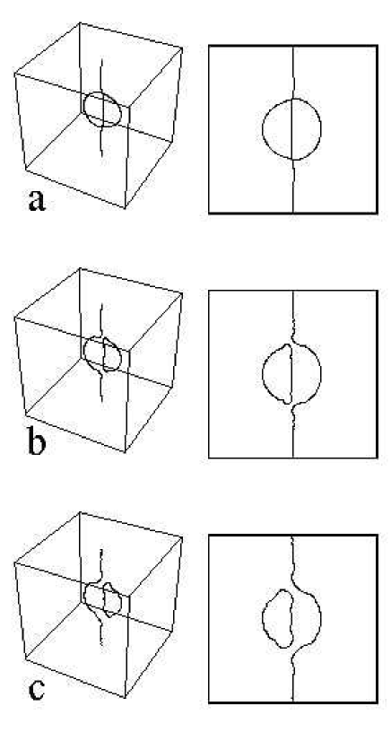
FIG. 1.: Collision of a straight vortex and a ring by the full Biot-Savart calculation without the mutual friction. The right column shows the side view of the left.

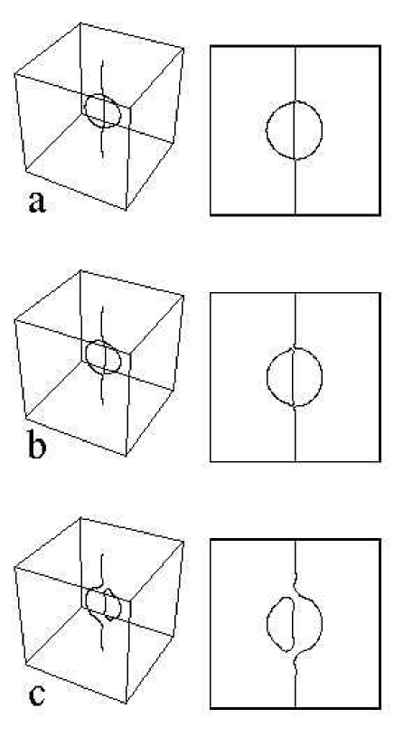
FIG. 2.: Collision of a straight vortex and a ring by the full Biot-Savart calculation with the mutual friction($\alpha=0.1$). The right column shows the side view of the left.

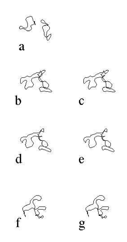
FIG. 3.: Typical motion of two vortices by the full Biot-Savart calculation. They approach(a), and reconnect(b) to be combined to one loop(c). Afterthat it is kinked(d) to cut off a small loop from itself(e). The same process occurs again((f) and (g)).

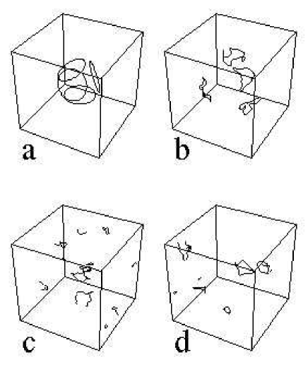
FIG. 4.: Motion of four vortex rings by the full Biot-Savart calculation without the mutual friction. The system is a 1cm³ cube and the periodic boundary conditions are used in all directions. The time is $t=0$s(a), 30s(b), 150s(c) and 500s(d).

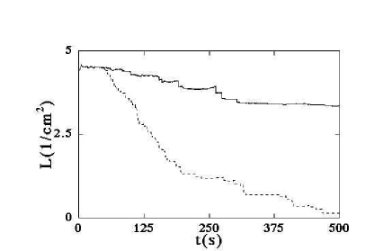
FIG. 5.: Decay of the VLD $L(t)$. The solid and dotted lines refer to the dynamics of Fig. 4 subject to the periodic boundary conditions and that of Fig.  7 confined by solid walls, respectively.

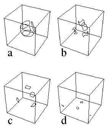
FIG. 6.: Motion of four vortex rings by the full Biot-Savart calculation with the mutual friction($\alpha=0.1$). The system is a 1cm³ cube and the periodic boundary conditions are used in all directions. The time is $t=0$s(a), 10s(b), 20s(c) and 40s(d).

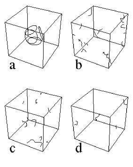
FIG. 7.: Motion of four vortex rings by the full Biot-Savart calculation without the mutual friction. The system is a 1cm³ cube and the system is confined by solid walls. The time is $t=0$s(a), 100s(b), 150s(c) and 300s(d).

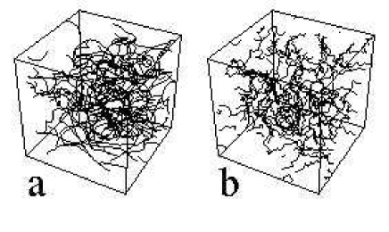
FIG. 8.: Example of a VT with (a) and without (b) the mutual friction.

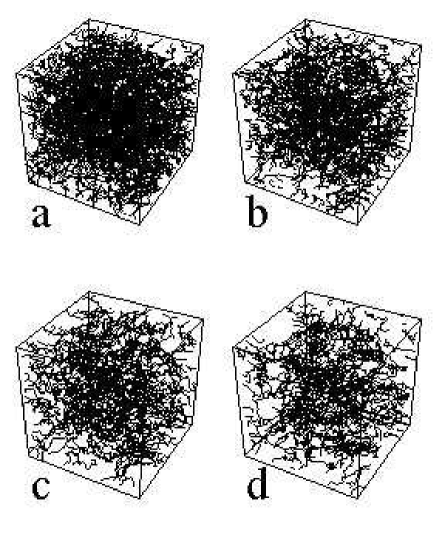
FIG. 9.: Decay of a dense VT by the LIA calculation without the mutual friction. The system is a 1cm³ cube. A periodic boundary condition is used only along the vertical direction in these figures, while the other sets of faces are treated as smooth, rigid walls. The time is $t=$0s(a), 30s(b), 60s(c) and 90s(d).

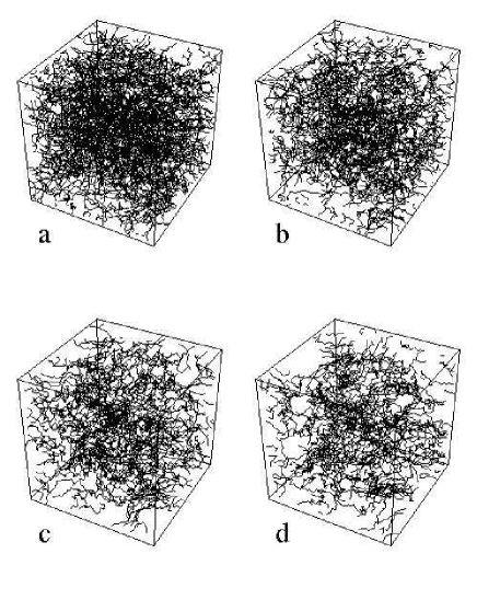
FIG. 10.: Decay of the VLD $L(t)$ for the dynamics of Fig.  9.

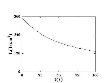
FIG. 11.: Comparison of the VLD decay for the different space resolutions $\Delta\xi=1.83\times 10^{-2}$cm (solid line) and its quarter (dotted line).

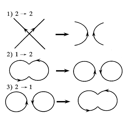
FIG. 12.: Kinds of reconnection. The type (1) shows two vortices reconnect to two. The type (2) is one vortex divides to two (the split type). The type (3) is two vortices are combined to one (the combination type).

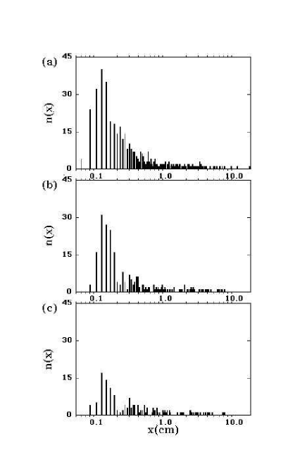
FIG. 13.: Bar chart showing the number of vortices $n(x)$ as a function of the length $x$ in the dynamics of Fig.  9. The range of $x$ is discretized by each $\Delta x=2\times 10^{-2}$cm. The time is $t=$0s(a), 50s(b) and 100s(c).

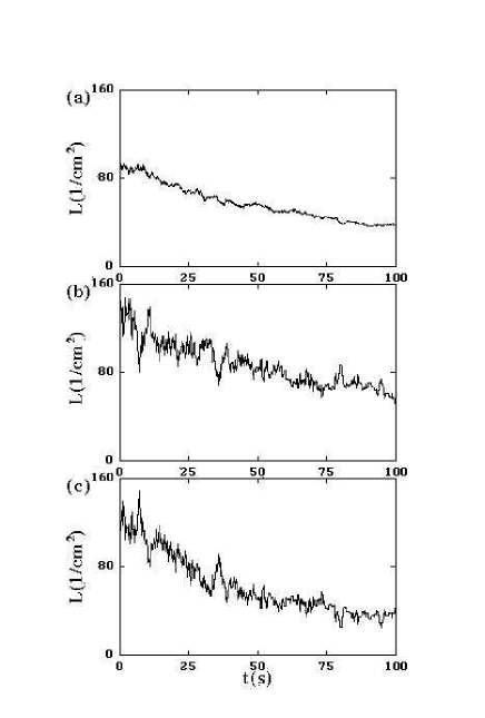
FIG. 14.: Contribution to the VLD from the vortices in the size range (a) $[\Delta\xi,a]$, (b) $[a,4a]$ and (c) $[4a-]$, where $a=1$cm.

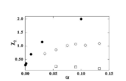
FIG. 15.: Dependence of $\chi_{2}$ on the mutual friction coefficient $\alpha$. The symbols $\bullet$ show the values obtained by this work, corresponding to $T=0$K, 0.91K, 1.07K, 1.26K, 1.6K, in order of increasing $\alpha$. The symbols $\circ$ denote the values observed by Vinen [5] when a heat current is suddenly switched on, and $\Box$ the values when a heat current is turned off. We used the relation $\alpha=B\rho_{n}/2\rho$  [2] in order to translate the Vinen’s data represented by another friction coefficient $B$.

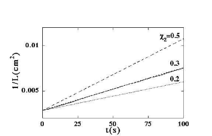
FIG. 16.: Comparison of the decay of $L(t)$ in Fig.  9 and the the solution (Eq. (23)) of the Vinen’s equation. The values of $\chi_{2}$ as a fitting parameter for Eq. (23) are shown in the figure.

TABLE I.: Classification of the reconnection events for each period in the VT dynamics of Fig.  9. See the text.

time(s)	total	split	comb.a	split/total($\%$)	comb./total($\%$)
0-10	1921	298	203	15.5	10.6
10-20	1366	252	161	18.4	11.8
20-30	1021	178	114	17.4	11.2
30-40	771	164	96	21.3	12.5
40-50	588	122	71	20.7	12.1
50-60	508	101	56	19.9	11.0
60-70	393	58	26	14.8	6.6
70-80	319	46	34	14.4	10.7
80-90	252	34	21	13.5	8.3
90-100	255	39	13	15.3	5.1
	7394	1292	795	17.5	10.8