Tunneling of Mesoscopic Spins in Molecular Crystals

1 Introduction

In small ferromagnetic nanoparticles, transitions between the magnetic states $\pm M$ generally occur by Thermal Activation (TA) over the anisotropy barrier. These transitions could also occur at constant energy by Quantum Tunneling (QT), with superposition of the two states $\pm M$. Magnetism being quantum at the atomic scale and classical at the macroscopic scale, a question raised in the past was to know what the size of a “giant spin” should be so that quantum manifestations could be observed (10, 10², 10³,$\dots\mu_{B}$). Early experiments devoted to this question showed that highly anisotropic rare-earth intermetallics, like Dy₃Al₂ and SmCo_3.5Cu_1.5, relax almost independently of temperature below a crossover temperature $T_{c}$ of a few Kelvin .${}^{\hbox{\immediate{\bf{?}})}}$ A “tunneling volume” of about 10²-10³ $\mu_{B}$ was obtained (equal to the thermal activation volume at $T_{c}$). These results and many others obtained more recently in the 90s on magnetic films and nanoparticles ,${}^{\hbox{\immediate{\bf{?}})}}$ are in agreement with today’s expectations for highly anisotropic systems, but the interpretations were difficult due to the presence of distributions of energy barriers. The first model describing thermal and quantum depinning of a narrow domain wall ,${}^{\hbox{\immediate{\bf{?}})}}$ was stimulated by the experiments on Dy₃Al₂ .${}^{\hbox{\immediate{\bf{?}})}}$ Recently, a clear demonstration of QT was obtained in the large spin molecules Mn₁₂-ac, and later in Fe₈. This allows to make a link between magnetism and mesoscopic physics, which is strengthened by a more recent study on the V₁₅ low spin molecule. In this paper, the phenomenon of Quantum Tunneling of Mesoscopic Spins is reviewed in the light of the behavior of the archetype of these systems: the molecular complex Mn₁₂-ac. This system is constituted of magnetic molecules containing 12 Mn ions with spins $3/2$ and 2, strongly coupled by super-exchange interactions. The resulting spin $S=10$ is relatively large and is defined over $\approx 1$ nm³, containing 10³ atoms of different species (Mn, O, C, H). The Hilbert space dimension is huge: 10⁸. However, in the “mesoscopic quantum tunneling approach” where the spin $S=10$ is assumed to be “rigid”, a Hilbert space dimension reduced to 21 is sufficient to understand most observations. Such a spin, in both Mn₁₂-ac and Fe₈, is large enough to exhibit an important energy barrier between the states $S=10$ and $S=-10$ in the presence of anisotropy (of e.g. uniaxial symmetry). This leads to extremely small tunnel splittings and slow relaxation. The latter can be decreased by orders of magnitude by the application of a longitudinal or transverse magnetic field. In Mn₁₂-ac, below 1 K, a longitudinal field of a few Tesla allows to observe tunneling between the states $m=-10$ and $m=10-n$ with $n=8$ to 11, while a transverse field of the same order shows ground-state tunneling ($m\approx-10$ to $m\approx 10$). The crossover temperature $T_{c}(H)$ between ground-state and thermally excited tunneling increases when the longitudinal field decreases. It extrapolates in zero field to the value $T_{c}(0)\approx 1.7$ K. This value confirms previous observations of a relatively high crossover temperature in bulk Mn₁₂-ac .${}^{\hbox{\immediate{\bf{?}},\penalty 1000\hskip 0.91003pt plus 0.70004pt minus 0.70004pt{\bf{?}})}}$ Finally, tunneling is deeply modified by environmental degrees of freedom and in particular by the spin bath which leads to a square root relaxation at short times.

In a second part of this paper the quantum behavior of a new molecule, so-called V₁₅, containing 15 spins $1/2$, is presented. The resultant spin $S=1/2$ is small, as a result of antiferromagnetic interactions. Contrary to high spin molecules, there is no energy barrier and the splitting between the symmetrical and anti-symmetrical states (given by the matrix element) is sufficiently large to allow spin-phonon transitions during spin rotation. In low spin molecules the coupling to the environment may be quite different from the one found in large spin molecules, unless the latter are with large non-diagonal matrix elements.

2 Large spin systems (Mn₁₂-ac type)

The subject of quantum tunneling in molecular crystals started with studies of the magnetic relaxation of oriented grains of Mn₁₂-ac .${}^{\hbox{\immediate{\bf{?}},\penalty 1000\hskip 0.91003pt plus 0.70004pt minus 0.70004pt{\bf{?}},\penalty 1000\hskip 0.91003pt plus 0.70004pt minus 0.70004pt{?},\penalty 1000\hskip 0.91003pt plus 0.70004pt minus 0.70004pt{\bf{?}},\penalty 1000\hskip 0.91003pt plus 0.70004pt minus 0.70004pt{\bf{?}})}}$ The relaxation time determined above 0.8 K follows an Arrhenius law $E=kT\ln(\tau/\tau_{0})$ with a prefactor $\tau_{0}\approx 10^{-7}-10^{-8}$ s and an energy barrier close to 60 K in zero field. Strong deviations to this behavior were observed below 2 K: in a field tilted by $45^{\circ}$, the relaxation tends to be independent of temperature .${}^{\hbox{\immediate{?},\penalty 1000\hskip 0.91003pt plus 0.70004pt minus 0.70004pt{?})}}$ This observation was interpreted as QT of the collective spin $S=10$. Furthermore, relaxation minima and dips in the ac-susceptibility, observed near zero field, suggested the phenomenon of resonant tunneling .${}^{\hbox{\immediate{?},\penalty 1000\hskip 0.91003pt plus 0.70004pt minus 0.70004pt{?})}}$

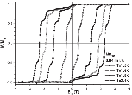
Fig.  1: Hysteresis loops of Mn₁₂-ac, with the field along the $c-$axis. Alternations of plateaus and steps suggest a “macroscopic quantization” of the longitudinal magnetization component. This in fact simply reminiscent of the quantization of $S_{z}$ of individual molecules $+$ tunneling in the presence of a complex environment.

Later, this phenomenon was quantitatively demonstrated by hysteresis loop measurements on oriented powder ${}^{\hbox{\immediate{\bf{?}})}}$ and on a single crystal .${}^{\hbox{\immediate{\bf{?}})}}$ Magnetization experiments done in higher fields and lower temperatures, led to similar conclusions .${}^{\hbox{\immediate{\bf{?}})}}$

2.1 Tunneling in a longitudinal magnetic field

For the description of the thermodynamical magnetic properties of Mn₁₂-ac, the reader could refer to ${}^{\hbox{\immediate{\bf{?}})}}$ and references therein.

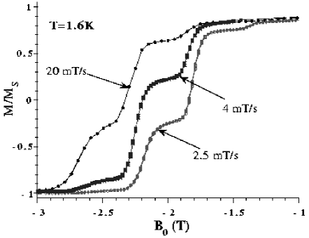
Fig.  2: Magnetization curves at different sweeping fields in Mn₁₂-ac.

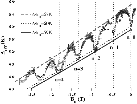
Fig.  3: Effective energy barrier of Mn₁₂-ac vs. a field along the $c-$axis, showing a parity effect. Values of the zero field barriers are given.

The out of equilibrium magnetic properties, are characterized by isothermal hysteresis loops measured on a single crystal of Mn₁₂-ac (Fig. 1). The field was applied along the $c-$easy axis of magnetization with a measuring timescale $\tau_{m}\approx 500$ s per data point .${}^{\hbox{\immediate{?})}}$ Below the blocking temperature of 3 K, staircases with equally separated magnetization steps characterize the dynamics of the system. In the flat portions of the loops, where the magnetization $M$ has not the time to relax, its relaxation time $\tau$ is such as $\tau_{m}\ll\tau$; in the steep portions of the loop where $M$ relaxes rapidly, $\tau_{m}\approx\tau$. As expected, faster sweeping rates give smaller and broader steps (see, in Fig. 2, the steps near 1.8 T; note that the last steps are always broader due to the “finite size” of the total magnetization). In addition, relaxation measurements give sharp minima precisely at the fields of the magnetization steps: $H_{n}\approx 0.44$ n, with $n=0,1,2,\dots$ ${}^{\hbox{\immediate{?})}}$ To illustrate this effect, we give here a dynamical scaling plot (Fig. 3) .${}^{\hbox{\immediate{?})}}$

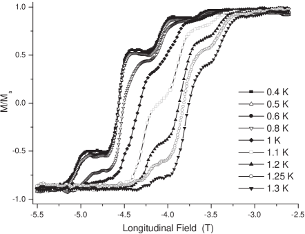
Fig.  4: Magnetization curves in decreasing field, extracted from torque measurements with an applied field parallel to the c-easy axis. One observes that below 0.6 K, the curves are temperature independent, showing that tunneling is not thermally activated.

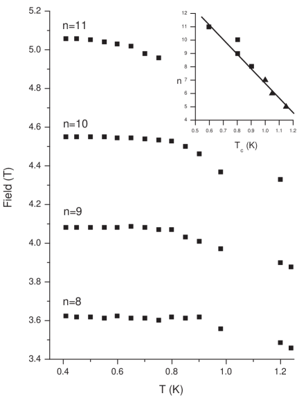
Fig.  5: Resonance fields $H_{n}$ measured for $n=8$, 9, 10, 11 at temperatures between 0.4 K and 1.25 K. For each $n$ a plateau is observed below a critical temperature $T_{c}(n)$. This temperature varies linearly with $n$ as shown in the inset: the triangles are plotted from A. Kent et al. ${}^{\hbox{\immediate{?})}}$ and the squares were obtained in our study.

Fig. 4 shows several hysteresis loops, recently measured at the High Magnetic Field Laboratory in Grenoble (LCMI), using a torque magnetometer below 1.3 K .${}^{\hbox{\immediate{\bf{?}})}}$ The way to extract the longitudinal magnetization (parallel to the easy $c-$axis) from the torque, will be published elsewhere and compared to previous experiments of Perenboom et al .${}^{\hbox{\immediate{?})}}$ In Fig. 4, the transverse component of the applied field was smaller than 0.1 T. The obtained hysteresis loops show magnetization jumps at certain values $H_{n}$ of the longitudinal field, as in Fig. 1, but the temperature being here rather low, the entire hysteresis loops become independent of temperature below a crossover temperature $T_{c}\approx 0.6$ K. This low temperature saturation, already observed,${}^{\hbox{\immediate{?})}}$ suggests that thermal activation is not relevant at these temperatures, and that tunneling takes place from the ground-state $m=-10$ to a state $m=10-n$, with $n=8$, 9, 10 and 11, depending on the exact value of $H_{n}$. These fields become independent of temperature below $T_{c}(n)$ but they decrease above this temperature (Fig. 5), confirming the existence of a crossover at $T_{c}$ (in the presence of fourth order crystal field terms). The inset of Fig. 5 shows that $T_{c}$ increases almost linearly when $n$, i.e. the field, decreases, as expected. Interestingly, a linear extrapolation of $T_{c}$ vs. $n$ gives the zero-field crossover temperature $T_{c}(0)\approx 1.7$ K. This value is consistent with the temperature of 1.9 K, below which the beginning of a relaxation plateau was observed ,${}^{\hbox{\immediate{?},\penalty 1000\hskip 0.91003pt plus 0.70004pt minus 0.70004pt{?},\penalty 1000\hskip 0.91003pt plus 0.70004pt minus 0.70004pt{\bf{?}})}}$ confirming the negligible role of the minority phase of Mn₁₂-ac at long time-scales .${}^{\hbox{\immediate{?},\penalty 1000\hskip 0.91003pt plus 0.70004pt minus 0.70004pt{?})}}$ A more detailed description of these experiments and their interpretation will be given in a further report.

2.2 Tunneling in a transverse magnetic field

In order to study the effect of a field perpendicular to the easy axis of magnetization, hysteresis loop measurements were first performed above 1.5 K with a field tilted by an angle $\theta$ .${}^{\hbox{\immediate{\bf{?}},\penalty 1000\hskip 0.91003pt plus 0.70004pt minus 0.70004pt{?})}}$ As for $\theta=0$, alternations of plateaus and steep variations of the magnetization $\Delta M$, are observed (Fig. 6). $\Delta M$ increases with the transverse field component $H_{T}=H\sin\theta$, but the positions of the steps remain at the same longitudinal field $H_{Ln}=H\cos\theta\approx{{\displaystyle{nD}}\over{\displaystyle{g\mu_{B}}}}$. Longitudinal and transverse fields having, to first order, “orthogonal” effects (the former puts the levels in coincidence and the latter removes the degeneracy of these coincidences by creating the tunnel splitting), it is normal that a transverse field does not modify significantly the coincidence if the applied field is much smaller than $H_{A}$, but only increases the tunneling probability. The measured relaxation times follow an Arrhenius law with a barrier reduced by the transverse field. The observed increase of $\Delta M$ with $H_{T}$ and $T$ is due to (i) easier TA resulting from the lowering of the energy barrier as predicted by the classical expression $\propto 1-2(H_{T}+H_{L})/H_{A}$ for $(H_{T}+H_{L})\ll H_{A}$ and/or (ii) easier QT resulting from the increase of the tunnel splitting of resonant level pairs $-m$ and $m-n$, $\Delta\propto(H_{T}/H_{A})^{2m-n}$ + higher terms. A comparison between these two contributions shows that thermally activated tunneling on excited states takes place on deeper and deeper energy levels when $H_{T}$ increases. The transmission rates of different thermally assisted channels in a transverse field were calculated  ${}^{\hbox{\immediate{?})}}$ and compared to experiments.

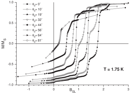
Fig.  6: Magnetization curves measured in Mn₁₂-ac with a tilted magnetic field (the angles are with the $c-$axis).

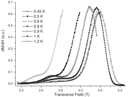
Fig.  7: Variation of $dM/dH$ vs. $H$, measured in Mn₁₂-ac with a transverse field of about 4 T. Below $\approx 0.6-0.7$ K, the curves are temperature independent.

It was concluded that ground-state tunneling is obtained for $H_{T}$ larger than a few Tesla. This effect was recently clearly shown for the first time. For that we made the same sub-Kelvin torque experiments as above, but in the presence of a field almost perpendicular to the easy $c-$axis of magnetization .${}^{\hbox{\immediate{?})}}$ In this case the symmetry of the double potential well of Mn₁₂-ac is essentially preserved and ground-state tunneling between the states $m\approx-10$ and $m\approx 10$ can be observed. In these experiments, the tilt angle was very close to $90^{\circ}$, within a range of one degree, giving a transverse field component between 3.5 and 4.5 T, and a longitudinal component varying around 0.04 T. Fig. 6 shows the $n=0$ resonance, observed in zero internal field. The longitudinal component of the applied field is exactly opposite to the Lorentz field, to cancel it. In order to show this resonance more clearly at different temperatures below 1.3 K, we plotted in Fig. 7 their profile $dM/dH$ vs. $H$. As observed in longitudinal fields, the curves are independent of temperature below a certain temperature, which is here $\approx 0.6-0.7$ K. This shows that below $T_{c}\approx 0.6-0.7$ K the tunneling, observed in zero internal field, is of pure quantum origin and corresponds to $m\approx-10$ to $m\approx 10$ transition. In particular phonon emissions which must be present in the case of asymmetrical potential wells are absent here and the relaxation plateau cannot be attributed to self-heating. Besides, thermalization is optimal in the ³He bath of these experiments. Note that the $m=-10$ and $m=10$ ground-states are in fact slightly mixed by the transverse field, and the $z$-component of $S$ in each well is reduced to a value which can be approximated by $m=S_{z}=\pm S\cos\phi\approx 9$ which is nevertheless close to 10 ($\phi$ is the angle between $S$ and the easy $c-$axis).

This first clear observation of ground-state tunneling of the main phase of Mn₁₂-ac allows to study the quantum relaxation of this system (next section). Note that in all these experiments with longitudinal and transverse fields of several Tesla, the minority phase of Mn₁₂-ac is superparamagnetic and cannot contribute to hysteresis loops and relaxation experiments, unless by increasing on a negligible way the dynamics through weak dipolar interactions.

3 Resonant tunneling mechanisms

3.1 General interpretation

The simplest way to interpret these results is to calculate the spectrum of energy levels in the presence of a magnetic field. For that we use the following Hamiltonian for a spin $S$ in a crystal field of tetragonal symmetry, with an applied field $\mbox{\boldmath$H$}(H_{x},H_{z})$. This Hamiltonian contains a diagonal part $H_{1}$ and a non-diagonal $H_{2}$ one :

$$H_{1}=-DS_{z}^{2}-BS_{z}^{4}-g\mu_{B}S_{z}H_{z}$$ (3.1)

and

$$H_{2}=-C(S_{+}^{4}+S_{-}^{4})-g\mu_{B}S_{x}H_{x}.$$ (3.2)

In so doing, one neglects all the internal degrees of freedom of the collective spin, and this is precisely the interest of this “mesoscopic” approach. With 4 spins $3/2$ and 8 spins 2, the dimension of the Hilbert space of the collective spin of Mn₁₂-ac is 10⁸ (or 6⁸ for Fe₈ and 2¹⁵ in V₁₅). Together with extremely small gaps, this very large dimensions can be taken as a characteristic of mesoscopic spins. Nevertheless we expect some effects associated with the fine structure of the molecule level in connection with e.g. intra-molecular anti-symmetric Dzyaloshinsky-Moryia interactions $\mbox{\boldmath$D$}_{ij}\cdot(\mbox{\boldmath$S$}_{i}\times\mbox{\boldmath$S$}_{j})$, which do not conserve $\mbox{\boldmath$S$}^{2}$  .${}^{\hbox{\immediate{?},\penalty 1000\hskip 0.91003pt plus 0.70004pt minus 0.70004pt{?})}}$ We assume that these terms are more or less well represented by different contributions in Eq. 3.1, 3.2. The energy spectrum in longitudinal field is given by the hamiltonian $H_{1}$, $E(m)=-Dm^{2}-Bm^{4}-g\mu_{B}mH_{z}$ where $m=S_{z}$. The levels $m(>0)$ and $n-m(<0)$ cross when $E(m)=E(n-m)$. The crossing fields (or resonance fields) are given by:

$$H_{n}={{\displaystyle{nD}}\over{\displaystyle{g\mu_{B}}}}[1+{{\displaystyle{B}}\over{\displaystyle{D}}}((m-n)^{2}+m^{2})].$$ (3.3)

If the effects of $B$ were neglected, the crossing fields would be equally separated and given by $H_{n}\approx nD/g\mu_{B}=nH_{A}/(2S-1)$, where $n=1,2,\dots$ The comparison with the observed sequence of fields $H_{n}\approx 0.44n$ gives $D/g\mu_{B}\approx 0.44$ T i.e. $D\approx 0.60$ K. The value $B/D\approx 0.002$ shows that the shift due to $B$ is small for excited levels but rather large for lowest levels. In the following we will take the set of values $D=0.56$ K, $B=1.1$ mK, $C=3\cdot 10^{-5}$ K obtained in EPR .${}^{\hbox{\immediate{\bf{?}})}}$ In low fields above 2 K, $\Delta H_{n}\approx 0.41(1+0.004m^{2})$ suggests that tunneling occurs mainly through $m\approx 4$. Energy barrier determination from relaxation measurements on the magnetization plateau near zero field gives $|E|\approx 67$ K. This is also in agreement with these parameters: for $n=0$, $E=-D_{eff}S^{2}$ with $D_{eff}=D+BS^{2}$ gives $E\approx 56+10^{-3}S^{4}\approx 67$ K (for $S=10$). Finally, direct anisotropy field measurements (magnetization measurement in a field perpendicular to the easy axis) give $|E|\approx 65$ K ${}^{\hbox{\immediate{?},\penalty 1000\hskip 0.91003pt plus 0.70004pt minus 0.70004pt{?})}}$ which is close enough to the EPR value of 67 K .${}^{\hbox{\immediate{?})}}$

The non-diagonal part of the hamiltonian $H_{2}$ removes the degeneracy at level crossings giving the splitting $\Delta$ (anti-crossing or level-repulsion). Following van Hemmen and Sütő ,${}^{\hbox{\immediate{\bf{?}})}}$ we can write for a non-diagonal term $C_{p}$ of order $p$:

$$\Delta(S,0)=\frac{DS}{\pi}\left(\frac{2DS^{2-p}}{C_{p}}\right)^{-2S/p}$$ (3.4)

The gap is an exponentially small fraction of the anisotropy level separation $\approx DS$ and is in general extremely small for large spins. This expression can be extended to $n\not=0$: $\Delta_{(m,n)}=(Dm/\pi)[(2D/C_{p})\cdot S^{(2-p)}\cdot f(m/S)]^{-(2m-n)/p}$ where $f(m/S)$ is a function which could be evaluated. The gaps $\Delta$ associated with the resonances allowed by the anisotropy $(-m,m^{\prime}=m-n,n)$ were calculated numerically in Mn₁₂-ac, by exact diagonalization of the $S=10$ matrix for the parameters given above (see Table I). Only those transitions such as $m-m\prime$ is a multiple of 4 are allowed. If a transverse field is also taken into account in the diagonalization, the condition becomes simply $m-m\prime=$ integer.

Table  I: Non-zero tunnel splittings calculated by exact diagonalization for the spin $S=10$ of Mn₁₂-ac. Each cell contains the splitting in Kelvin and the label of the crossing levels under the form $(-m,m^{\prime},n)$. The crystal field parameters ${}^{\hbox{\immediate{?})}}$ are given in section 3.1.

(-10,10,0)	(-10,6,4)	(-10,2,8)	(-10,-2,12)	(-10,-6,16)
$1.15\cdot 10^{-11}$	$4.67\cdot 10^{-8}$	$1.61\cdot 10^{-5}$	$1.84\cdot 10^{-3}$	$9.67\cdot 10^{-2}$
(-9,7,2)	(-8,8,0)	(-8,4,4)	(-8,0,8)	(-8,-4,12)
$9.41\cdot 10^{-8}$	$1.16\cdot 10^{-7}$	$7.45\cdot 10^{-5}$	$8.68\cdot 10^{-3}$	$2.98\cdot 10^{-1}$
(-9,3,6)	(-7,5,2)	(-6,6,0)	(-6,2,4)	(-6,-2,8)
$4.19\cdot 10^{-5}$	$1.03\cdot 10^{-4}$	$1.14\cdot 10^{-4}$	$1.77\cdot 10^{-2}$	$4.97\cdot 10^{-1}$
(-9,-1,10)	(-7,1,6)	(-5,3,2)	(-4,4,0)	(-4,0,4)
$4.69\cdot 10^{-3}$	$1.33\cdot 10^{-2}$	$2.08\cdot 10^{-2}$	$2.2\cdot 10^{-2}$	$6.38\cdot 10^{-1}$
(-9,-5,14)	(-7,-3,10)	(-5,-1,6)	(-3,1,2)	(-2,2,0)
$1.94\cdot 10^{-1}$	$4.02\cdot 10^{-1}$	$4.97\cdot 10^{-1}$	$6.76\cdot 10^{-1}$	$6.89\cdot 10^{-1}$

As an example, $H_{x}=0.1$ T gives $\Delta/k_{B}=2$ mK for $m=m\prime=3$. The fast increase of $\Delta$ with $n$ explains why a longitudinal field allows to observe the relaxation of Mn₁₂-ac below 1 K. The gaps also increase dramatically with a transverse field as shown by Eq. 3.4.

3.2 Tunneling probability between two levels

If the two levels were exactly in coincidence the tunneling rate would simply be given by $\Delta/h$. However this situation never occurs because levels are never in “static coincidence”. If one assumes that a magnetic field is applied with the rate $c=dH/dt$ at the anti-crossing of two levels, the time $\Delta/cg\mu_{B}S$ during which the field crosses the region $\Delta/g\mu_{B}S$ where the magnetic states are mixed, can be much smaller or much larger than the characteristic oscillation time of the two-level system $h/\Delta$. In the first limit, the initial spin state $S_{z}=-m$ has not enough time to mix with $S_{z}=m-n$ and it is unchanged (non adiabatic transition). In the second one, $-m$ changes in $m-n$ and at the anti-crossing the two states are mixed giving oscillations of $S_{z}$ (adiabatic case). In this intermediate region, $S_{z}=0$. In the general case ${}^{\hbox{\immediate{\bf{?}},\penalty 1000\hskip 0.91003pt plus 0.70004pt minus 0.70004pt{\bf{?}},\penalty 1000\hskip 0.91003pt plus 0.70004pt minus 0.70004pt{\bf{?}},\penalty 1000\hskip 0.91003pt plus 0.70004pt minus 0.70004pt{\bf{?}})}}$ (Landau-Zener model) the transition probability is given by the ratio of these two times:

$$P_{m,n}=1-\exp\left({-\Gamma_{m,n}}\right)$$ (3.5)

with

$$\Gamma_{m,n}=\pi\Delta_{(m,n)}^{2}/[2\hbar(2m-n)g\mu_{B}dH/dt]$$ (3.6)

If $\Gamma_{m,n}\ll 1$, $P_{m,n}\approx\Gamma_{m,n}$. In large spin systems such as Mn₁₂-ac or Fe₈ where zero-field ground-state splittings $\Delta/g\mu_{B}S$ are of the order of 10^-9 and 10^-11 T, the regions $\Delta$ are crossed in 10${}^{-9}/c$ to 10${}^{-11}/c$ seconds. The oscillation time $h/\Delta$ is going from 10^-3 to 0,1 second, the Landau-Zener probabilities are $\Gamma\approx 10^{-6}/c$ and 10${}^{-10}/c$, (where $c$ is expressed in T/s). Typical values of $c$ (between 10^-3 and 10³ T/s) give $\Gamma\ll 1$ i.e. essentially non-adiabatic Landau-Zener transitions (in the absence of fluctuations and magnetic field). It is clear that with an applied field, $\Delta$ can reach values approaching $P\approx 1$ (Eq. 3.4), and this is the reason why ground-state tunneling can easily be observed in Mn₁₂-ac, as shown above.

3.3 Effects of temperature

For a given coincidence field ($n$ fixed), $-m$ can take different values $-m=-10,-9,\dots$ up to the top of the barrier. A tunneling channel can be associated with each one of these values of $-m$, giving paths such as $-S\Rightarrow-m\Rightarrow m\Rightarrow S$. The first portion ($-S\Rightarrow-m$) is thermally activated while the second one ($-m\Rightarrow m$) is tunneling. The third one ($m\Rightarrow S$) is associated with phonon emissions. The total transition rate is given by the product of the Thermally Activated rate $\Gamma(m)=\tau_{0}^{-1}\exp{(E(-S)-E(-m))/kT}$ by the tunneling probability $P_{m,n}$ between $-m$ and $m-n$:

$$\Gamma_{TA}=P_{m,n}\tau_{0}^{-1}\exp{(E(-S)-E(-m))/kT}$$ (3.7)

This expression explains the Arrhenius behavior of the relaxation time in the high temperature regime of Mn₁₂-ac. In this regime, tunneling simply modifies the prefactor of the Arrhenius law (whose temperature dependence is weak compared to the exponential). Depending on the values of temperature and field, three different tunneling regimes can be defined:

$-$ The thermally activated tunneling regime, where tunneling takes place on upper paths. These paths are on levels $m<m_{c}$, for which the tunneling probability is much larger than the thermal one, i.e. $P_{m,n}\approx 1$. This high temperature regime allows to understand the passage to the classical behavior. The rate for $-m$ to $m-n$, change is given by:

$$\Gamma_{Ac}\approx\tau_{0}^{-1}\exp{(E(-S)-E(-m_{c}))/kT}$$ (3.8)

Above $E(m_{c})$, the barrier is transparent: tunneling is so fast that it short-circuits the top of the barrier at energies larger than $E(m_{c})$. One can see in Eq. 3.4 that for small $m$, $\Delta$ becomes comparable to crystal field level separations and everything is so well mixed that the states of spins up and down have no meaning (there is no barrier). In the presence of a longitudinal field, one can also define an “effective barrier”:

$$E(m,n)=E_{eff}(H)\approx E_{eff}(0)(1-H/H_{A})^{\alpha},$$ (3.9)

with

$$E_{eff}(0)=E(-m_{c})-E(-S)\approx D_{eff}(S^{2}-m_{c}^{2})$$

The notion of effective barrier $E_{eff}(H)$ has the advantage to provide a simple scaling expression (Eq. 3.8 and Eq. 3.9) for the analysis of relaxation experiments in the thermally activated tunneling regime. The relaxation times $\tau(H,T)$ measured in Mn₁₂-ac between 2.5 and 3 K have been analyzed using the scaling plot of $E_{eff}=T\ln\tau(H,T)$, with $\alpha\approx 2$ or $3/2$ (Fig. 3). The effect of tunneling is equivalent to a reduction of energy barrier from 67 K to 60 K (in zero field), i.e. of about $10\%$. A comparison with (Eq. 3.9) gives $(m_{c}/S)^{2}\approx 0.1$, and this shows that tunneling short-circuits the top of the barrier when $m\leq m_{c}\approx 3$. Interestingly, ac-susceptibility experiments give $E\approx 64$ K ,${}^{\hbox{\immediate{?},\penalty 1000\hskip 0.91003pt plus 0.70004pt minus 0.70004pt{?})}}$ and this is a larger value than the 60 K of quasi-static experiments because ac-experiments are faster, giving smaller reduction of the top of the barrier. This scaling analysis is more accurate than previous plots. It shows dips in $E_{eff}$ which are more important for even values of $n$ than for odd ones. This parity effect seems to be a tunneling manifestation of the fourth order transverse anisotropy terms $C(S_{+}^{4}+S_{-}^{4})$ which contributes to tunneling only for $n$ even or multiple of 4 (depending on the parity of m). In fact it is very general, in particular because it occurs not only for fourth order terms but also for other orders, such as the order one if the timescale is short enough .${}^{\hbox{\immediate{?},\penalty 1000\hskip 0.91003pt plus 0.70004pt minus 0.70004pt{\bf{?}})}}$ As an example, in the presence of a transverse magnetic field, even resonances are induced by $S_{+}^{4}$ or $S_{-}^{4}$, whereas odd resonances are induced by combinations like by $S_{x}S_{+}^{4}$ or $S_{x}S_{-}^{4}$ .${}^{\hbox{\immediate{\bf{?}})}}$ It is clear that these effects, observed here at high temperature, also exist at low temperature.

$-$ The thermally assisted tunneling regime is for intermediate paths. The TA probability $\propto\exp({-D_{eff}(S^{2}-m_{c}^{2})/kT})$ and the tunneling one are not very different from each other. This is for $m>m_{c}\approx 3$, but not too large, otherwise levels are too deep and tunneling is too slow. The thermally assisted tunneling rate for $-m$ to $m-n$ transitions can be written:

$$\Gamma_{As}\approx\Gamma_{0}\exp{(D_{eff}(S^{2}-m_{c}^{2}))/kT},$$ (3.10)

with

$$\Gamma_{0}={{\displaystyle{\pi\Delta^{2}}}\over{\displaystyle{2\hbar g\mu_{B}(2m-n)h_{s}}}}\frac{\tau_{s}}{\tau_{0}}$$

if $\tau_{0}\ll\tau_{s}$, where $h_{s}$ and $\tau_{s}$ are the amplitude and the characteristic time of internal field fluctuations, and $\tau_{0}$ the prefactor of the Arrhenius law. In the presence of dipolar field distribution $\Gamma_{0}$ is multiplied by $h_{s}/H_{D}$ where $H_{D}$ is the width of the distribution .${}^{\hbox{\immediate{\bf{?}})}}$ The tunneling gap can be evaluated by a comparison of measured and calculated relaxation rates (Eq. 3.10). In assisted tunneling regime, where $\tau\approx 10^{6}$ s, at $T\approx 2$ K, $H\approx 0$, $\tau_{0}\approx 10^{-8}$ s and $H_{D}\approx 40$ mT and $\tau_{s}=T_{1}\approx 10^{-4}$ s (see below), we find $\Delta/k_{B}\approx 3$ mK. This value is close to the gap $\Delta/k_{B}\approx 2$ mK, calculated for $m=m_{c}\approx 3$ (Table I). For $m>3$ or 4, $\Delta$ decreases dramatically (Eq. 3.4 or Table I), and relaxation times become very long ($\Gamma_{0}\propto\Delta^{2}$). In order to observe ground-state tunneling it is necessary to increase level mixing by applying a magnetic field.

$-$ The Ground-State tunneling regime. In the presence of a longitudinal field, the tunneling path $-S$ to $+S-n$ is followed by phonon emissions while $+S-n$ reaches the ground-state $+S$. In the absence of longitudinal field ($n=0$), tunneling occurs between $-S$ and $+S$ (ground-state tunneling). Energy conservation is naturally fulfilled, but couplings to the environment are still required for angular momentum conservation. In both cases tunneling rate can be enhanced by the application of a transverse field. At $T=0$ the tunneling rate is given by (for $\Gamma\ll 1$):

$$\Gamma_{GS}=P_{(-S,S-n)}/\tau_{s}=\pi\Delta_{(S,n)}^{2}/[2\hbar g\mu_{B}(2S-n)H_{D}]$$ (3.11)

where is $H_{D}$ the internal dipolar field ($g\mu_{B}SH_{D}=E_{D}$). Here too the comparison between measured and calculated relaxation times gives access to the tunnel splitting. The relaxation time measured in zero field at 1.8 K (beginning of the plateau), $\tau\approx 10^{9}$ s ,${}^{\hbox{\immediate{?},\penalty 1000\hskip 0.91003pt plus 0.70004pt minus 0.70004pt{?},\penalty 1000\hskip 0.91003pt plus 0.70004pt minus 0.70004pt{?})}}$ gives $\Delta/k_{B}\approx 10^{-10}$ K .${}^{\hbox{\immediate{?})}}$ This value is not very much different from $\Delta/k_{B}\approx 10^{-11}$ K, calculated by diagonalization for $S=10$ (Table I). A value of $C\approx 4.5\cdot 10^{-5}$ K instead of $3\cdot 10^{-5}$ K could explain this difference.

Using more recent relaxation experiments below 1.3 K and in the presence of a transverse field of 4 T, we find a tunnel splitting of $\Delta/k_{B}\approx 10^{-5}$ K (section 4.3).

3.4 Effects of environment

The crucial role of couplings to the environment in “Macroscopic Quantum Tunneling” was pointed out several years ago .${}^{\hbox{\immediate{\bf{?}})}}$ These couplings tend to destroy MQT effects, but at the same time they are necessary to observe it. Environmental couplings giving dissipation, the spin motion between the two wells is non-equally damped, and this dephases the two wave functions and destroys their interferences: the system becomes more classical and tunneling is eventually suppressed. In Ref  ${}^{\hbox{\immediate{?})}}$ we gave a physical picture of this effect, called “topological decoherence” ,${}^{\hbox{\immediate{\bf{?}},\penalty 1000\hskip 0.91003pt plus 0.70004pt minus 0.70004pt{\bf{?}})}}$ in terms of the Berry phases .${}^{\hbox{\immediate{\bf{?}})}}$

Tunneling can also be suppressed if the environment contains internal bias fields, which brings the molecules out of coincidence. The main origins of internal fields are the quasi-static components of hyperfine fields of the molecule itself and the quasi-static components of dipolar fields between molecules. They give a Zeeman energy distribution for molecular spins. The Zeeman shifts of the states $+m$ and $-m$ of a molecule with non-zero internal field, can be compensated by the application of an external field of opposite value. However this compensation cannot be exact due to finite field resolution $\delta H$, (unless $g\mu_{B}S\delta H<\Delta$, which is unrealistic for mesoscopic spins). This basic interdiction for tunneling can be lifted by the environment, and in particular by fast fluctuations of internal fields. If the energy separation of the levels $+m$ and $-m$, is smaller than $g\mu_{B}mH_{f}$ where $H_{f}$ is the amplitude of the fluctuating field, these levels will come into coincidence $1/\tau_{f}$ times per second, where $\tau_{f}$ is the mean fluctuation time, allowing tunneling at each coincidence in the “energy window ” $g\mu_{B}mH_{f}$. This effect of dynamical (homogeneous) broadening “averaging” static inhomogeneous broadening, in a given energy window was recognized only recently .${}^{\hbox{\immediate{?})}}$ In this work the fluctuations were assumed to be of hyperfine origin: the fast fluctuations of amplitude $H_{f}$ are those of the hyperfine fields and their characteristic time is $\tau_{f}=T_{2}$. However at large enough temperature, the temperature dependent process $T_{1}$ or fast fluctuations of the dipolar fields can also be relevant.

Note that the applied field itself is never completely stable and its fluctuations about a stable mean value can induce tunneling. This seems to be an interesting aspect of the measurement in quantum mechanics, where fluctuations in the measuring apparatus induce tunneling (here the coils, the current supply). In an ideal system where the environment would only be constituted of the measurement set up without any other fluctuations tunneling could only be observed through the imperfections of the measuring tool. The width of the tunnel transition would be simply given by the instrumental homogeneous broadening of quantum levels, allowing tunneling in the window $g\mu_{B}m\sqrt{<h^{2}>}$, where $\mbox{\boldmath$h$}(t)$ is the fluctuating part of the field $H$ conjugated to the order parameter. Further analysis will require to distinguish between our ability to select a given value of the applied field and the uncertainty on the determination of this value. Note that one may simulate a “bad measuring tool”, by applying a fluctuating field of amplitude larger than the internal fields. The simplest case, which we use commonly, is to apply an ac field to accelerate the dynamics, but the simulation of a “bad apparatus” would require to apply a field random in time (e.g. white noise) and to test the effect of different statistics on the resultant tunneling effect (amplitude, time-scale, white noise or with correlations ).

In systems such as Mn₁₂-ac or Fe₈, hyperfine and dipolar field fluctuations are in general more important than those of the measuring tool. When the temperature is such that the first excited level $m=9$ is occupied (roughly above 1 K), fast fluctuations come from local dipolar and hyperfine fields $H_{loc}$ around their mean values, with $\Delta I=\Delta m=\pm 1$ co-flips ($T_{1}$), and also at higher temperature from phonon transitions associated with $\Delta m=\pm 1$. At low temperature when these process are frozen, only $T_{2}$ remains. The dominant fluctuation time given by an Orbach process ${}^{\hbox{\immediate{\bf{?}})}}$ is $T_{1}\approx\tau_{0}\exp(E(m)-E(S))/k_{B}T$ and $H_{f}\approx H_{loc}/S\approx H_{loc}/I\sqrt{N}$. For Mn₁₂-ac at about 2 K, we get $T_{1}\approx 10^{-4}-10^{-5}$ s and $H_{f}\approx 1-5$ mT ($S=10$, $I=5/2$ and $N=12$ for the Mn nuclear spins in a molecule). NMR on Mn nuclear spin was recently made possible by Goto et al .${}^{\hbox{\immediate{\bf{?}})}}$ Transfered hyperfine fields of protons give $T_{1}\approx 10^{-4}$ s and $H_{f}\approx 1.4$ mT .${}^{\hbox{\immediate{\bf{?}})}}$

4 Relaxation laws and resonance profile

There are two ways to describe a resonance. In the first one, one plots the profile of the resonance determined at a given time-scale, e.g. by plotting $dM/dH$ vs. $H$, for a given sweeping field rate $dH/dt$. In the second one, the field is kept constant and one plots the magnetization vs. time, $M(t)$. Both ways were studied in Mn₁₂-ac. It was shown that relaxation laws $M(t)$ and resonance profile $dM(H)/dH$ are not independent.

4.1 Thermally activated relaxation

In the high temperature regime, above $\approx 2.5$ K i.e. not far from $T_{B}$, the tunnel splitting $\Delta$, averaged over a few excited levels, is of the order of the resonance line-width (about 0.5 K). In this case the resonance, homogeneously broadened by spin-phonon transitions of energy $\Delta$, has a Lorentzian line-shape and the relaxation is exponential ($M\propto\exp(-t/\tau)$). The contribution of dipolar fields to the resonance line-width is also Lorentzian, because any “reaction” of dipolar fields $H_{D}$ to spin reversals, is continuously averaged in time, meaning that the system is equilibrated. The tunnel window covers the whole resonance and since $g\mu_{B}H_{D}\approx\Delta$, the resonance width is of both origins (dipolar and intrinsic i.e. with spin-phonon transitions). This equilibrated regime, corresponds to what we called above the “thermally activated tunneling” regime.

4.2 Thermally assisted relaxation

In the intermediate temperature regime (below $\approx 2.5$ K), dipolar fields are essentially frozen leading to an inhomogeneous distribution of internal fields. The intrinsic tunnel window of width $\Delta$ and the small fluctuating parts of internal fields are much narrower than the width of the inhomogeneous distribution of internal fields: the latter is not averaged by the quantum dynamics and its profile could be anything (e.g. Gaussian in particular theoretical situations, but numerical simulations showed that it is in general more complex than either Lorentzian or Gaussian). In Mn₁₂-ac at 1.6 K, resonance peaks are shifted to lower fields and their width increases after zero-field cooling, showing that the inhomogeneous distribution of dipolar fields is at this temperature broad enough to determine the resonance width ${}^{\hbox{\immediate{?})}}$).

In this intermediate temperature regime, strong deviations from exponential relaxation were observed, and in particular a square root law .${}^{\hbox{\immediate{\bf{?}},\penalty 1000\hskip 0.91003pt plus 0.70004pt minus 0.70004pt{?})}}$

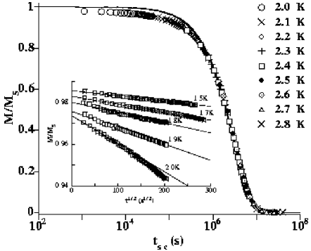
Fig.  8: Scaling plot of the relaxation in Mn₁₂-ac in zero applied field. Strong deviations from an exponential occur below $t_{sc}\approx 10^{6}$ s (continuous curve). The scaling variable is $\tau_{sc}=(t+t_{w})\cdot\tau(2$ K$)/\tau(T)$, where $\tau$ is the relaxation time and $t_{w}$ is an experimental waiting time. Inset: low temperature regime where the relaxation is nearly a square root of the time.

However this law is not limited to 0 K and $M\approx M_{s}$ as predicted. Furthermore a crossover between square root and exponential relaxation is quite apparent in Mn₁₂-ac. A scaling analysis (Fig. 8) shows (i) an asymptotic exponential regime between 3 K and $\approx 2.7$ K (high-temperatures / long-times), (ii) important deviations from this regime between $\approx 2.5$ and 2 K, and finally (iii) a square root asymptotic regime below 2 K (low-temperatures / short-times). This low temperature regime was recently extended down to 0.4 K (see below). The crossover region (ii) is broad and not trivial. In particular it shows highly non-linear S-shaped $M(t)$ curves. Furthermore, it takes place at temperatures where Mn₁₂-ac should be equilibrated, with exponential relaxation. These observations seem to result from the decrease of the total magnetization $M(T,t)$, with increasing time or/and $T$ .${}^{\hbox{\immediate{?})}}$ In this case, the mean internal field decreases, and this leads to opposite shifts of the spin-up and spin-down density of states. The first resonance (in zero internal field) is maximum when the applied field compensates the mean internal field (Lorentz field): $H_{0}=-H_{int}=-CM(T,t)$, where $C=4\pi/3-N$ gives the difference between the Lorentz field and the sample demagnetizing field. If the sample has a needle shape, as in Mn₁₂-ac, this field $H_{1}\approx-4\pi M(T,t)/3$, is negative. In other systems with different shapes, like Fe₈, it is positive. In the course of relaxation the $+S$ density of states decreases (due to the decrease of $H_{1}(t,T)$) and this gives also a square root relaxation, but which is valid at high temperature i.e. in the thermally assisted regime (at low temperatures where the changes in $M(t,T)$ are too small, the square root regime is exclusively described in the frame of model ${}^{\hbox{\immediate{?})}}$ ). Furthermore the relaxation law may depend on whether the relaxation is performed exactly at resonance or not. This allows in particular to understand the not trivial $S$-shaped relaxation curves.

4.3 Ground-state relaxation

The hysteresis loops shown above, deduced from torque experiments in the presence of relatively large longitudinal and transverse fields, give evidence of temperature-independent tunneling below $\approx 0.6$ K (Fig. 4 and Fig. 5). Now we consider the relaxation experiments performed in the same conditions of field and temperature, i.e. around 4 T and at temperatures below 1.3 K. This will make a link with previous experiments above 1.5 K, and fields up to 3 T. In both cases of longitudinal and transverse field, the observed quantum relaxation can be very fast and this allows to analyze in details the $M(t)$ curves even at temperatures well below 1 K.

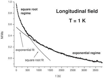
Fig.  9: Relaxation curve in a longitudinal field for the resonance $n=8$ ($H\approx 4$ T) and $T=1$ K. The square root regime is observed only at short timescales, then the relaxation becomes exponential.

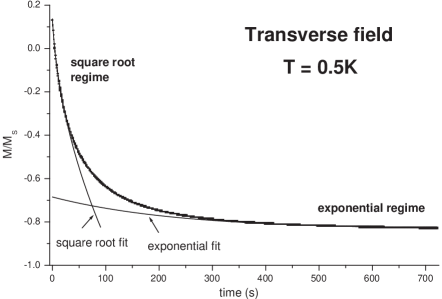
Fig.  10: Relaxation curve in a transverse field of 4 T for the resonance $n=0$ and $T=0.5$ K. The square root regime is observed only at short timescales, then the relaxation becomes exponential.

Two examples of relaxation curves measured in a longitudinal or a transverse field are plotted in Fig. 9 and Fig. 10. A square root regime is clearly observed in both cases, but at short timescales only (see also Fig. 11). At longer timescales, the relaxation becomes exponential in all cases. In these figures the square root and exponential plots are done using the following expressions:

$$(M-M_{i})/M_{s}=\sqrt{\Gamma(t+t_{0})}$$ (4.1)

and

$$(M-M_{e})=A\exp{-(\Gamma^{\prime}t)}$$ (4.2)

Note that the data are much more noisy in longitudinal. This is because in this case the torque is minimum (a very small transverse field component has to be set to get a torque), while in the transverse case it is almost maximum. Nevertheless, the square root and exponential character of the relaxations is evident in both cases.

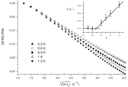
Fig.  11: Magnetic relaxation in Mn₁₂-ac for $n=0$ (transverse field), plotted vs. the square root of time $t+t_{0}$ where $t_{0}=1.5$ s is imposed by our experimental time resolution. The weak S-shaped character of the curve is due to small shifts in the density of spin states with temperature (see section 4.2). In the inset is plotted the deduced square root relaxation time for different temperatures. One notes a plateau below $0.6-0.7$ K.

The square root relaxation time derived from short timescale experiments is plotted in the inset of Fig. 10. It is independent of temperature below a crossover temperature $T_{c}$ of about $0.6-0.7$ K, showing ground-state tunneling relaxation in the bulk phase of Mn₁₂-ac for the first time. The observed square root law, being for $n=0$, corresponds to the switch of the total magnetization from $+M_{s}$ to $-M_{s}$ and it is centered near $M=0$, i.e. for $M\ll M_{s}$, which was not predicted in model.${}^{\hbox{\immediate{?})}}$ It is interesting to note that the crossover temperature $T_{c}(H)$ between ground-state and thermally assisted tunneling does not seem to be related to the crossover temperature $T_{b}(H)$ between square root and exponential relaxation. The reason is that the former depends only on the temperature of the spin bath while the second depends also on the equilibration of the spin-phonon system with the cryostat temperature.

Contrarily to the experiments performed at $T>2$ K and discussed above, the square root laws observed below 1 K are not associated with the shift of the total energy distribution of spins, but results from a hole burned by tunneling in this energy distribution at zero energy, as predicted by Prokof’ev and Stamp.${}^{\hbox{\immediate{?})}}$ This hole must persist during all the square root regime (about 30 seconds) and should vanish in the exponential regime which characterizes an equilibrated spin system. The existence of such a finite hole life-time below $T_{c}$ cannot be predicted in a zero Kelvin model. At finite temperature the hole should vanish when the spin system becomes equilibrated, i.e. when the tunnel window becomes as large as the width of quasi-static internal field distribution. This is what is in principle expected above $T_{c}$. The fact that this is observed even below $T_{c}$, at long timescales, suggests that there are other mechanisms such as spin-phonon transitions which reorganize the spin energy distribution at temperatures below $T_{c}$.

Let us now evaluate the ground-state tunneling gap $\Delta$, from the relaxation experiments in longitudinal and transverse fields of $\approx 4$ T.

In the first case, the tunneling rate is given by $\Gamma=\pi\Delta^{2}/(2\hbar E_{D})$ where $E_{D}=(2S-n)g\mu_{B}H_{D}$. Knowing the measured rate $\Gamma\approx 10^{-3}s^{-1}$, $S=10$, $n=8$, $g\mu_{B}H_{D}/k_{B}\approx 0.05$ K, this expression gives $\Delta/k_{B}\approx 10^{-5}$ K. Interestingly the calculation of the splitting, by diagonalization, using the anisotropy constants of Mn₁₂-ac up to fourth order, gives a value which is very close, $\Delta/k_{B}=1.6\cdot 10^{-5}$ K (Table I).

In the second case, the tunneling rate is given by the same expression where $E_{D}=2Sg\mu_{B}H_{D}$. Taking $g\mu_{B}H_{D}/k_{B}=0.05$ K, the measured rate $\Gamma\approx 10^{-2}$ s^-1 gives $\Delta/k_{B}\approx 4\cdot 10^{-5}$ K. The diagonalization of the matrix gives $\Delta/k_{B}\approx 10^{-5}$ K. Note that when $\Gamma\tau_{s}\approx 1$ the fast tunneling rate should be written $[1-\exp{(-\pi\tau_{s}\Delta^{2}/2\hbar E_{D})]}/\tau_{s}$. This expression shows that $\tau_{s}$ plays effectively a role in the tunneling rate, but only if $\Gamma\tau_{s}\approx 1$. This is not the case in general, where slow relaxation leads to the expression used above $\Gamma\approx(\pi\Delta^{2})/(2\hbar E_{D})$. We conclude that ground-state relaxation is only sensitive to changes in hyperfine fluctuations characteristic time. At moderately high temperatures where $\tau_{0}<\tau_{s}\approx(T_{1},T_{2})$, the situation is different and $\tau_{s}$ might play a role in the relaxation as shown in Eq. 3.10. Finally, the slope $dn/dT_{c}$ in the inset of Fig. 5 allows to evaluate the mean $\Delta$ for $5<n<11$. We find $\Delta/k_{B}\approx 1.5\cdot 10^{-6}$ K.

Although much larger than in zero field, these gaps are still too small to be perturbed by spin-phonon transitions. These transitions are relevant in the thermally activated regime only. As discussed above, this restriction does not apply to magnetic fluctuations of e.g. nuclear spins: a fluctuating field of only $10^{-3}$ T would spread the Landau-Zener transition over 20 mK, i.e. 2000 times $\Delta$. This is why the spin bath, with fluctuations of amplitude $h_{s}$ and characteristic time $\tau_{s}$ ($c_{s}\approx h_{s}/\tau_{s}$), plays a dominant role to induce tunneling. This is true unless $dH/dt$ is much faster than hyperfine fluctuations. The condition for coherent adiabatic Landau-Zener transition is $\Delta^{2}/\hbar g\mu_{B}S\gg c\gg c_{s}$.

Finally, if there are no phonons with energy comparable to the tunneling gap $\Delta\ll k_{B}T$, a large number of phonons must be available at the energy scale of the hole width, and this explains why (i) non-equilibrated square root behavior is observed even above $T_{c}$ at short timescales, (ii) equilibrated exponential behavior is observed even below $T_{c}$ at long timescales.

5 Low spin systems (V₁₅ type)

The process of spin reversal in this system has been studied by dynamical magnetization experiments in the sub-Kelvin temperature range .${}^{\hbox{\immediate{\bf{?}})}}$

In the molecular complex $K_{6}[V_{15}^{IV}As_{6}O_{42}(H_{2}O)]\cdot 8H_{2}O$ (so-called V₁₅) ${}^{\hbox{\immediate{\bf{?}})}}$ all intra-molecular exchange interactions being antiferromagnetic, the total spin of the molecule is $S=1/2$; there is no energy barrier and no tunneling. However the physics of spin rotation has some similarities with the case of large spin molecules.

In Fig. 12 where three hysteresis loops are presented at three different temperatures for a given sweeping rate, the plateau is higher and more pronounced at low temperature. The same tendency is observed at a given temperature and faster sweeping rate (Fig. 13). When compared to its equilibrium limit (dotted curve in Fig. 13), each magnetization curve shows a striking feature: the plateau intersects the equilibrium curve and the magnetization becomes smaller than at equilibrium. Equilibrium is then reached in higher fields near saturation.

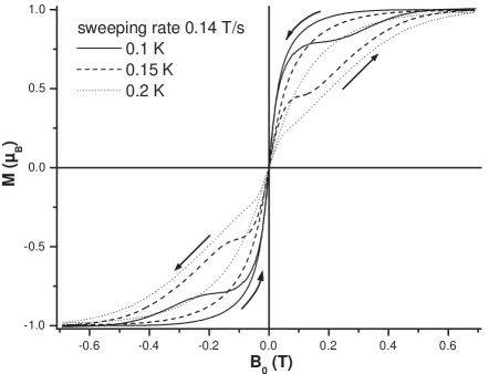
Fig.  12: Measured hysteresis loops for three temperatures and for a given field sweeping rate 0.14 T/s. The plateau is more pronounced at low $T$.

In order to interpret this magnetic behavior of the V₁₅ molecules, we will analyse how the level occupation numbers vary in this two level system when sweeping an external field. In the absence of dissipation, a 2-level model is well described by the bare Landau-Zener model, in the adiabatic or non-adiabatic case (low or high sweeping rates). The probability for the $|1/2,-1/2\rangle\leftrightarrow|1/2,1/2\rangle$ transition is $P=1-\exp(-\pi\Delta_{0}^{2}/4\hbar\mu_{B}c)$. In such a Landau-Zener transition, the plateaus of Fig. 12,13 should decrease if the sweeping rate increases, which is contrary to the experiments. Taking the typical value $c=0.1$ T/s and the zero-field splitting $\Delta_{0}/k_{B}\approx 0.05$ K  ,${}^{\hbox{\immediate{?})}}$ one gets a ground state switching probability very close to unity: in the absence of dissipation the spin 1/2 must adiabatically follow the field changes. But, dissipation due to spin-phonon coupling make the transition dissipative (or non-adiabatic, from the thermodynamical point of view). The mark of the $V_{15}$ system is that this coupling is acting also near zero applied field because $\hbar\omega\approx\Delta_{0}$ is of the order of the bath temperature, which is not the case of large spin molecules where $\Delta_{0}\ll k_{B}T$.

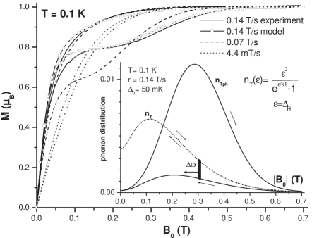
Fig.  13: Measured hysteresis loops for three field sweeping rates at $T=0.1$ K. The observed plateau is more pronounced at high sweeping rate. The square-symbol curve was calculated with the model discussed in text. We find a good agreement between model and experiment. In the inset the calculated number of phonons with $\hbar\omega\approx\Delta_{0}$ is plotted vs. the sweeping field modulus (note the arrows) at equilibrium (dotted line) and out-of-equilibrium (black line). The difference between the two curves (thick segment $\Delta_{0}$) suggests the moving hole in the phonon distribution, while their intersection gives the plateau intercept of the equilibrium magnetization curve.

In a direct process, the spins at the temperature $T_{S}$ should relax to the phonon temperature within a timescale $\tau_{1}$, the phonons being at the bath temperature. However, even with a silver sample holder, it is not possible to maintain the phonon temperature equal to the temperature of the bath. This is because in V₁₅ below 0.5 K, the heat capacity of the phonons $C_{ph}$ is very much smaller than that of the spins $C_{S}$, so that the energy exchanged between spins and phonons will very rapidly adjust the phonon temperature $T_{ph}$ to the spin one $T_{S}$. Furthermore, the energy is transferred from the spins only to those phonon modes with $\hbar\omega=\Delta_{H}$ (within the resonance line width), where $\Delta_{H}$ is the two level field-dependent separation. The number of such lattice modes being much smaller than the number of spins, energy transfer between the phonons and the sample holder must be very difficult, a phenomenon known as the phonon bottleneck  .${}^{\hbox{\immediate{\bf{?}})}}$ If this phonon density of states does not equilibrate fast enough, the hole must persist and move with the sweeping field, leading to a phonon bottleneck. This means that the spin system will not be able to get the equilibrium, as soon as an external field is swept with a sufficiently large rate. Let us note that in zero field the system is out-of-equilibrium even if magnetization passes through the origin of coordinates. At larger fields, in the plateau region, the level population is almost constant at timescales shorter than $\tau_{H}$, even after the plateau crosses the equilibrium curve. Equilibrium is reached when $\tau_{H}$ becomes small enough.

In ${}^{\hbox{\immediate{?})}}$ we give a theoretical model inspired from the well-known work of Abragam & Bleaney  .${}^{\hbox{\immediate{\bf{?}})}}$ Starting from the balance equations of the coupled spin-phonon two level system, we derive the relaxation law of the magnetic moment: $-t/\tau_{H}=x(t)-x(0)+\ln((x(t)-1)/(x(0)-1))$, where $x(t)$ is the deviation of the magnetization from its equilibrium. $\tau_{H}$ is the relaxation time and is a function of field and temperature (see  ${}^{\hbox{\immediate{?},\penalty 1000\hskip 0.91003pt plus 0.70004pt minus 0.70004pt{?})}}$). We then calculate the hysteresis loops with very realistic values of the parameters and we find a good agreement between measurements and the calculus of hysteresis loops and relaxation times.

The V₁₅ molecular complex constitutes an example of dissipative two-level system of mesoscopic size. The total spin 1/2 being formed of a large number of interacting spins, its splitting results from the structure itself of the molecule (intra-molecular hyperfine and Dzyaloshinsky-Moriya couplings) and it is rather large (a fraction of Kelvin). In V₁₅ and in other low-spin systems, splittings must be much larger than in large-spin molecules where the presence of energy barriers lowers them by orders of magnitude (e.g. $10^{-11}$ K in Mn₁₂, see above). This is the reason why spin-phonon transitions are important in low-spin molecules and not relevant in high-spin ones, unless a large transverse field is applied (it increases the tunnel splitting and probability) in which case we would also expect similar phenomena.

6 Conclusion

The evidence of resonant tunneling of the magnetization in Mn₁₂-ac allows to make a link between magnetism and mesoscopic physics. In particular it shows that the transition between the low temperature quantum behavior and the high temperature classical one, takes place through an intermediate regime in which tunneling is thermally assisted. These studies also shed light on the effects of spin couplings with their environment. The magnetic relaxation law $M(t)$ and resonance line-shape $dM/dH$ are connected to each other. They both give different results depending on the strength of the coupling with the bath : square root relaxation and any type of line-shape when the spin (and phonon) system is not at equilibrium, and exponential relaxation with Lorentzian line-shape when it is equilibrated. However, this is not an absolute rule and we found, and explained, situations where a square root relaxation can be also observed when the spin system is at equilibrium. These results obtained previously above 1.5 K are confirmed by high fields sub-kelvin experiments. In particular the crossover between square-root and exponential relaxation law at $T_{b}$, and the crossover between ground-state and thermally activated tunneling at $T_{c}$, are clearly observed in the bulk phase of Mn₁₂-ac. Note that these two crossovers do not coincide. This observation is not surprising because the former is related to different couplings with the bath (spins, phonons), while the latter is essentially a single molecule effect. Finally, we have evaluated the tunneling gaps of the bulk phase of Mn₁₂-ac for different experimental cases. A very good agreement was always obtained with the gaps obtained by exact diagonalization.

The role of spin-phonon transitions is discussed in details in the low spin molecule V₁₅, where the absence of barrier leads to large gaps. This study, in which the reversal of a “macroscopic” spin $1/2$ is analyzed, shows particular hysteresis loops reminiscent but definitely different from those of high spin molecules. The hysteresis loop of low spin molecules comes from spin-phonon transitions. It is concluded that in the presence of a large magnetic field, spin-phonon transitions should also be important in large spin molecules and lead to hysteresis loops similar to these observed in V₁₅.

References

- [1] M. Uehara and B. Barbara: J. Phys. 47 (1986) 235 and refs. therein.
- [2] L. Gunter, B. Barbara (Eds.): Quantum Tunneling of Magnetization, NATO ASI series E: Applied Sciences 301, Kluwer, Dordrecht (1995).
- [3] T. Egami: Phys. Stat. Sol. B 57 (1973) 211; ibid. A 19 (1973) 747; 20 (1973) 57.
- [4] B. Barbara: Proc. 2nd Int. Symp. on Anisotropy and Coercivity 137 (1978); J. de Phys. 34 (1977) 1039; Sol. State Com. 10 (1972) 1149 .
- [5] C. Paulsen, J. G. Park, B. Barbara, R. Sessoli, A. Caneschi: J. Magn. Magn. Mat. 140-144 (1995) 1891.
- [6] C. Paulsen, J. G. Park, B. Barbara, R. Sessoli, A. Caneschi: J. Magn. Magn. Mat. 140-144 (1995) 379.
- [7] B. Barbara et al.: J. Magn. Magn. Mater. 140-144 (1995) 1825.
- [8] C. Paulsen and J. G. Park: in p. 189.
- [9] M. A. Novak and R. Sessoli: in p. 171.
- [10] J. R. Friedman, M. P. Sarachik, J. Tejada, R. Ziolo: Phys. Rev. Lett. 76 (1996) 3830. J. M. Hernandez, X. X. Zhang, F. Luis, J. Bartolome, J. Tejada, R. Ziolo: Europhys. Lett. 35 (1996) 301.
- [11] L. Thomas, F. Lionti, R. Ballou, R. Sessoli, D. Gatteschi and B. Barbara: Nature 383 (1996) 145.
- [12] J. A. A. J. Perenboom, J. S. Brooks, S. Hill, T. Hathaway and N. S. Dalal: Phys. Rev. B 58 (1998) 333.
- [13] B. Barbara, L. Thomas, F. Lionti, I. Chiorescu, A. Sulpice: J. Magn. Magn. Mat. 200 (1999) 167.
- [14] I. Chiorescu, R. Giraud, A. Caneschi, A. G. M. Jansen, B. Barbara: to be published.
- [15] B. Barbara, L. Thomas, F. Lionti, A. Sulpice, A. Caneschi: J. Magn. Magn. Mat. 177-181 (1998) 1324.
- [16] L. Thomas, A. Caneschi, B. Barbara: Phys. Rev. Lett. 83 (1999) 2398.
- [17] F. Lionti, L. Thomas, R. Ballou, B. Barbara, A. Sulpice, R. Sessoli, D. Gatteschi: J. Appl. Phys. 81 (1997) 4608.
- [18] A. L. Barra, D. Gatteschi, R. Sessoli: Phys. Rev. B 56 (1997) 8192 .
- [19] J. L. van Hemmen and A. Sütő: in pg. 19.
- [20] S. Miyashita: J. Phys. Soc. Jap. 64 (1995) 3207; J. Phys. Soc. Jap. 65 (1996) 2734.
- [21] L. D. Landau: Phys. Z. Sowjetunion 2 (1932) 46. C. Zener: Proc. R. Soc. London A 137 (1932) 696.
- [22] L. Gunther: EuroPhys. Lett. 39 (1997).
- [23] V. V. Dobrovitski, A. K. Zvezdin: Europhys. Lett. 33 (1997) 377.
- [24] D. A. Garanin and E. M. Chudnovsky: Phys. Rev. B 56 (1997) 11102.
- [25] I. Tupitsyn, B. Barbara: to be published.
- [26] A. J. Leggett et al.: Rev. Mod. Phys. 59 (1987) 1; Lectures in Phys., Les Houches (1986). A. J. Leggett: in p. 1; A. O. Caldeira and A. J. Leggett: Phys. Rev. Lett. 46 (1981) 211. P. C. E. Stamp: 61 (1988) 2905; N. Prokof’ev and P. C. E. Stamp: J. of Low Temp. Phys. 104 (1996) 143; J. of Phys. Cond. Matt. 5 (1993) L663.
- [27] P. C. E. Stamp, E. Chudnovsky and B. Barbara: Int. J. of Mod. Phys. B 9 (1992) 1355.
- [28] P. C. E. Stamp: Phys. Rev. Lett. 61 (1988) 2905.
- [29] P. M. V. Berry: Proc. R. Soc. London A 392 (1984) 45.
- [30] N. V. Prokof’ev and P. C. E. Stamp: Phys. Rev. Lett. 80 (1998) 5794 and J. of Low Temp. Phys. 113 (1998) 1147.
- [31] J. Villain, F. Hartmann-Boutron, R. Sessoli, A. Rettori: Europhys. Lett. 27 (1994) 159; P. Politi, A. Rettori, F. Hartmann-Boutron, J. Villain: Phys. Rev. Lett. 75 (1995) 537; F. Hartmann-Boutron, P. Politi, J. Villain: Int. J. Mod. Phys. B 10 (1996) 2577; M. Leuenberger and D. Loss: Europhys. Lett. 46 (1999) 692.
- [32] T. Goto, T. Kubo, T. Koshiba, Y. Fujii, A. Oyamado, J. Arai, K. Takeda, K. Awaga: preprint sep.1999, to appear in Physica B (2000).
- [33] A. Lascialfari, Z. H. Jang, F. Borsa, P. Carretta and D. Gatteschi: Phys. Rev. Lett. 82 (1998) 3773.
- [34] T. Ohm, C. Sangregorio and C. Paulsen: J. of Low Temp. Phys. 113 (1998) 1141.
- [35] L. Thomas and B. Barbara: J. of Low Temp. Phys. 113 (1998) 1055.
- [36] I. Chiorescu, W. Wernsdorfer, A. Müller, H. Bögge and B. Barbara: Phys. Rev. Lett. 84 no.15 (2000).
- [37] A. Müller, J. Döring: Angew. Chem. Int. Ed. Engl. 27 (1991) 1721. D. Gatteschi, L. Pardi, A. L. Barra, A. Müller, J. Döring: Nature 354 (1991) 465.
- [38] J. H. Van Vleck: Phys. Rev. 59 (1941) 724. K. W. H. Stevens: Rep. Prog. Phys. 30 (1967) 189.
- [39] A. Abragam, B. Bleaney: Electronic Paramagnetic Resonance of Transitions Ions, Clarendon Press - Oxford, chap. 10, (1970).
- [40] A. D. Kent, Y. Zhong, L. Bokacheva, D. Ruiz, D. N. Hendrickson, M. P. Sarachik: EuroPhys. Lett. 49 (4) (2000) 521.