Efficient Monte Carlo algorithm and high-precision results for percolation

Abstract

We present a new Monte Carlo algorithm for studying site or bond percolation on any lattice. The algorithm allows us to calculate quantities such as the cluster size distribution or spanning probability over the entire range of site or bond occupation probabilities from zero to one in a single run which takes an amount of time scaling linearly with the number of sites on the lattice. We use our algorithm to determine that the percolation transition occurs at $p_{c}=0.59274621(13)$ for site percolation on the square lattice and to provide clear numerical confirmation of the conjectured $4/3$-power stretched-exponential tails in the spanning probability functions.

Published as Phys. Rev. Lett. 85, 4104–4107 (2000).

Percolation [1] is one of the best studied problems in statistical physics, both because of its fundamental nature and because of its applicability to a wide variety of different systems. Percolation models have been used as a representation of resistor networks [2], forest fires [3], epidemics [4], biological evolution [5], and social influence [6], as well as, of course, percolation itself. The word percolation appears in the title of almost four thousand physics papers in the last quarter of a century.

Numerical studies of percolation are straightforward by comparison with many simulations in statistical physics because no Markov process is needed to perform importance sampling. One can generate a single correct sample from the ensemble of possible states of a site (bond) percolation model on any lattice simply by populating each of the sites (bonds) of that lattice independently with occupation probability $p$. Typically one then finds all the connected clusters of occupied sites (bonds) in the resulting configuration using either depth-first or breadth-first search, and uses this information to calculate some observable of interest, such as average or largest cluster size. An extension of this method is the well-known Hoshen–Kopelman algorithm [7], which allows one to find all the clusters while storing the state of only a small portion of the lattice at any time. Other numerical algorithms have been developed to answer specific questions about percolation models, such as the hull-generation algorithm [8, 9], which can tell us whether a cluster exists which spans a square lattice with open boundary conditions without actually populating all the sites of that lattice first.

All of these algorithms have one feature in common: they tell us about the properties of the system for one specified value of $p$ only. In most cases one would like to know about the properties of the system over a range of values anywhere up to the entire domain $0\leq p\leq 1$. Although $p$ can in theory take any real value in this range, we need not, on a system of finite size, study an infinite number of values of $p$ to answer a question about that system with arbitrary precision. In fact, on a system of $N$ sites, we need measure an observable $Q$ only for systems having a fixed number $n$ of occupied sites (or bonds). We will refer to this as the “microcanonical ensemble” for the percolation problem. If we can measure the values $Q_{n}$ of our observable for all $0\leq n\leq N$ (or the equivalent range for bond percolation), then we can find the value $Q(p)$ for the more common “canonical ensemble” for any value of $p$ by convolution with a binomial distribution:

$$Q(p)=\sum_{n}\left({N\atop n}\right)p^{n}(1-p)^{N-n}Q_{n}.$$ (1)

Both depth-first and breadth-first searches take time ${\rm O}(N)$ to construct all clusters, and since there are ${\rm O}(N)$ possible values of the number of occupied sites or bonds, it is therefore possible to calculate $Q(p)$ over the entire range of $p$ in time ${\rm O}(N^{2})$. The hull-generating algorithm can perform the same calculation marginally faster, in time ${\rm O}(N^{15/8})$, but is, as mentioned above, restricted to measuring only certain observables such as the existence (or not) of a system-spanning cluster. Histogram interpolation methods [10] can reduce the time taken for a general measurement to ${\rm O}(N^{3/2})$, at the cost of a reduction in numerical precision, while the position of the percolation point can be found in time ${\rm O}(N\log N)$, by performing a binary search among the $N$ possible values of $n$ [1, 11].

In this paper we present a new algorithm which can find the value of a quantity or quantities over the entire range of $p$ from zero to one in time ${\rm O}(N)$—an enormous improvement over the simple ${\rm O}(N^{2})$ algorithm described above. As a corollary, the algorithm can also find the position of the percolation point in time ${\rm O}(N)$, since one can consider the existence (or not) of a spanning cluster to be the observable of interest. Our algorithm calculates the value of the quantity or quantities of interest for all values of $n$ in the microcanonical ensemble described above and the value in the canonical ensemble can then be calculated by employing Eq. (1). We describe the algorithm first for the bond percolation case, which is slightly simpler than site percolation.

The basic idea behind our algorithm is the following. We start with a lattice in which no bonds are occupied, and hence every site is a separate cluster. Each of these single-site clusters is given a unique label (e.g., a positive integer) by which we identify it. We then fill in bonds on the lattice in random order. When a bond is added to the lattice it either connects together two sites which are already members of the same cluster—in which case we need do nothing—or it connects two sites which are members of two different clusters. In this second case we must change the labels of one of the clusters to reflect the fact that the new bond has amalgamated the two. In order to accomplish this efficiently, we store the clusters using a tree-structure in which one site in each cluster is chosen to be the “root node” of that cluster and contains the cluster label. All other sites in the cluster possess pointers which point either to the root node, or to another site in the cluster, such that by following a succession of such pointers one can get from any site to the root node. This scheme is illustrated for the case of the square lattice in Fig. 1a. (A similar scheme is used in the Hoshen–Kopelman algorithm [7].) Clusters can now be efficiently amalgamated simply by adding a pointer from the root node of one to the root node of the other (dotted arrow in the figure), thereby making the former a sub-tree of the latter [12].

Our algorithm consists of repeatedly adding a random bond to the lattice, identifying the clusters to which the sites at its ends belong by traversing their respective trees until we find the root nodes, and then, if necessary, amalgamating the two trees. Generically, this kind of algorithm is known as a “union–find” algorithm in the computer science literature. Our implementation for the percolation problem uses the “weighted union–find with path compression” [13], in which (a) two trees are always amalgamated by making the smaller a sub-tree of the larger (“weighting”) and (b) the pointers of all nodes along the path traversed to reach the root node are changed to point directly to the root (“path compression”). Tarjan [14] has shown for this algorithm that the average number of steps taken to traverse the tree is proportional to $\alpha(n)$, where $\alpha$ is the functional inverse of Ackermann’s function and $n$ is the number of nodes in the tree. This in turn implies that the number of steps is effectively constant as the tree becomes large. Our simulations confirm this result, the constant taking a value of about $3.6$ on the square lattice, for example. The computation time taken in all other parts of the algorithm is also constant, and thus the time taken for each bond to be added is ${\rm O}(1)$ and the time taken to add all $N$ bonds is ${\rm O}(N)$. Hence we can construct clusters for all values of $n$ in one run of length ${\rm O}(N)$.

The weighting in the tree union algorithm requires that we know the number of nodes in each cluster. This is easy to arrange however: we store the cluster sizes at the root nodes of the clusters and when two clusters are amalgamated we simply add their cluster sizes together.

In order to actually measure some quantity of interest we usually have to do some additional work. For example, if we wish to measure largest cluster size we need to keep a running score of the largest cluster seen so far, as the algorithm progresses. If we wish to measure the position of the percolation point, we can do so by adding variables to each site in a cluster which store the displacement to the “parent” node in the tree. Then when we traverse the tree, we add these displacements together to find the total displacement to the root node. When we add a bond to the lattice which connects together two sites which belong to the same cluster, we calculate the two such displacements and take their difference. On a lattice with periodic (toroidal) boundary conditions percolation has not occurred if this difference is equal to a single lattice unit, otherwise it has—see Fig. 1b. (The same technique has been used to find the percolation point of Fortuin–Kasteleyn clusters in the Potts model [15].)

For site percolation, the algorithm is very similar to the one for the bond case just described. Sites are added in random order, and each one added either forms a new detached cluster in its own right, joins onto a single neighboring cluster, or joins together two or more extant clusters. The clusters are stored in a tree structure as before, and overall operation takes time ${\rm O}(N)$.

We have tested our algorithm for both site and bond percolation on square lattices of $L\times L$ sites with $L$ up to $10\,000$. The time taken for one run of our algorithm is found to scale as $N^{\alpha}$ with $\alpha=1.02\pm 0.04$, in agreement with the expected value of $\alpha=1$. Even for the largest systems, a single run takes only about 100 seconds on current computers. Larger systems still would be easily within reach but we are limited by the amount of memory available. This is not an important issue, however, since statistical error, rather than finite-size scaling, is the principal factor limiting the accuracy of our numerical results, making it more sensible to spend resources on reducing these errors than on simulating especially large systems.

In this paper we apply our algorithm to the calculation of the probability $R_{L}(p)$ for a cluster to wrap around the periodic boundary conditions on a square lattice of $L\times L$ sites with site percolation. For large $L$ this probability is equal to the probability that the system percolates. Since cluster wrapping can be defined in a number of different ways there are a corresponding number of different probabilities $R_{L}$. Here we consider the following: $R_{L}^{(h)}$ and $R_{L}^{(v)}$ are the probabilities of wrapping horizontally or vertically around the system respectively; $R_{L}^{(b)}$ is the probability of wrapping around both directions simultaneously; $R_{L}^{(e)}$ is the probability of wrapping around either direction; and $R_{L}^{(1)}$ is the probability of wrapping around one direction but not the other. (Note that configurations which wrap around both directions are taken to include both those which wrap directly around the boundary conditions and “spiral” configurations in which a cluster wraps around both directions before joining up.) For the square systems considered here, these probabilities satisfy the relations:

$$R_{L}^{(h)} = R_{L}^{(v)},$$ (2)

$$R_{L}^{(e)} = R_{L}^{(h)}+R_{L}^{(v)}-R_{L}^{(b)}=2R_{L}^{(h)}-R_{L}^{(b)},$$ (3)

$$R_{L}^{(1)} = R_{L}^{(h)}-R_{L}^{(b)}=R_{L}^{(e)}-R_{L}^{(h)}=\mbox{$\frac{1}{2}$}\bigl{(}R_{L}^{(e)}-R_{L}^{(b)}\bigr{)},$$ (4)

as well as the inequalities $R_{L}^{(b)}\leq R_{L}^{(h)}\leq R_{L}^{(e)}$ and $R_{L}^{(1)}\leq R_{L}^{(h)}$.

Most previous studies of $R_{L}(p)$ have examined the probability of a cluster connecting the boundaries of open systems. The work presented here differs from these studies by focusing on wrapping probabilities for periodic systems, and constitutes the first precise such study. As we will show, the use of wrapping probabilities yields estimates of the position of the percolation threshold with much smaller finite-size corrections than open-boundary methods.

To measure the wrapping probability we perform a number of runs of the algorithm to find the number of occupied sites $n$ for which cluster wrapping first occurs in the appropriate direction. Then the corresponding $R_{L}$ within the microcanonical ensemble is simply the fraction of runs for which that point falls below $n$. Convolving the resulting curve with a binomial according to Eq. (1) then gives us $R_{L}$ within the canonical distribution. Figure 2 shows $R_{L}$ for each of the four definitions above for a variety of system sizes. Note that $R_{L}^{(1)}$ in frame (d) is non-monotonic, since the probability of wrapping around one direction but not the other tends to zero as $p\to 1$.

The exact values of $R_{L}$ at percolation for each of the definitions above have been derived by Pinson [16, 17], and are $R_{\infty}^{(h)}(p_{c})=0.521058290$, $R_{\infty}^{(e)}(p_{c})=0.690473725$, $R_{\infty}^{(b)}(p_{c})=0.351642855$, and $R_{\infty}^{(1)}(p_{c})=0.169415435$. We can use these figures to measure the value of $p_{c}$, which is not known exactly for site percolation on the square lattice, by finding the value of $p$ for which $R_{L}(p)=R_{\infty}(p_{c})$. These estimates turn out to scale particularly well with system size. For each of the definitions of $R_{L}$ we find numerically that the difference $R_{L}(p_{c})-R_{\infty}(p_{c})$ scales approximately as $L^{-2}$. Since the width of the critical region scales as $L^{-1/\nu}$, this implies that our estimates of $p_{c}$ in finite systems should have a leading order finite-size correction which goes as $L^{-2-1/\nu}=L^{-11/4}$. This represents a very rapid convergence, in contrast to the $L^{-1/\nu}$ behavior of typical percolation estimates (such as RG estimates) and the $L^{-1-1/\nu}$ of certain open-system estimates [18], which is the best previously known convergence. Note that if the microcanonical values of $R_{L}$ are used instead of the canonical ones, the difference $R_{L}(p_{c})-R_{\infty}(p_{c})$ scales as $L^{-1/2}$, making this method significantly inferior to the one described above.

The non-monotonic probability function $R_{L}^{(1)}(p)$ is never equal to $R_{\infty}^{(1)}(p_{c})$ because the value of $R_{L}^{(1)}$ on systems of finite size is less than the value at $L=\infty$. However, in this case we can estimate $p_{c}$ from the position of the maximum of the function, and this estimate is also expected to scale as $L^{-2-1/\nu}$.

In Fig. 3 we show the values of $p_{c}$ estimated from our Monte Carlo results as a function of $L^{-11/4}$ for $L=32$, $64$, $128$, and $256$ for each of the four definitions of $R_{L}$. At least $3\times 10^{8}$ runs were carried out for each system size to achieve high statistical accuracy. Two different random number generators were used: a two-tap 32-bit additive lagged Fibonacci generator with taps at 418 and 1279, and a four-tap 32-bit XOR generator with taps at 471, 1586, 6988 and 9689. Allowing for statistical fluctuation, results were consistent between generators.

The best fits to $L^{-11/4}$ give estimates for the position of the percolation threshold for site percolation on the square lattice of $0.59274621(13)$ for $R_{L}^{(h)}$, $0.59274636(14)$ for $R_{L}^{(e)}$, $0.59274606(15)$ for $R_{L}^{(b)}$, and $0.59274629(20)$ for $R_{L}^{(1)}$. Our best estimate of $p_{c}$ is therefore

$$p_{c}=0.59274621\pm 0.00000013,$$ (5)

which is more accurate by a factor of four than the best previously published estimate of this quantity [18, 19] and should prove useful for high-precision studies of percolation in the future.

While it is encouraging to be able to estimate $p_{c}$ so accurately, the real power of our algorithm lies in its ability to efficiently estimate a function such as $R_{L}(p)$ over the entire range of $p$. To demonstrate the application of this idea, we have used our simulations to extract explicit evidence of the expected $\frac{4}{3}$-power tail in the logarithm of the cluster wrapping probability function.

The probability $R_{L}(p)$ that a given realization of a percolation model will wrap around a finite lattice at a particular value of $p$ is expected to go as $\exp(-L/\xi)$ when $\xi\ll L$ [11, 20]. Putting $\xi\sim(p_{c}-p)^{-\nu}$ we thus get

$$R_{L}\sim\exp(-L(p_{c}-p)^{\nu}).$$ (6)

This variation with $p$ is difficult to detect using standard algorithms for measuring $R_{L}$ (see, for example, Ref. [11]), since one needs to generate large numbers of samples at many different values of $p$, and almost all of that work will be wasted, since most of the systems simulated do not percolate. Our algorithm however shows the behavior of Eq. (6) clearly without further work. Equation (6) implies that a plot of $\log(-\log R_{L})$ against $\log(p_{c}-p)$ should have an asymptotic slope of $\nu=\frac{4}{3}$. In the inset of Fig. 3 we show such a plot for the functions $R_{L}^{(h)}$ and $R_{L}^{(b)}$ for systems with $L=256$. The $\frac{4}{3}$-power tail is clearly visible.

To conclude, we have presented a new Monte Carlo algorithm for studying site or bond percolation on any lattice. The algorithm is capable of measuring the entire curve of an observable quantity as a function of the occupation probability $p$ in a single run taking time of order the volume of the system. We have also proposed a new and highly accurate method for measuring the position of the percolation threshold by calculating the probabilities for clusters to wrap around the boundary conditions on a toroidal system. We have used this method in combination with our Monte Carlo algorithm to find the value of $p_{c}$ for site percolation on the square lattice to greater accuracy than any previously published calculation. In addition we have used our algorithm to demonstrate clearly the presence of the expected $\frac{4}{3}$-power tails in the logarithm of the cluster wrapping probability.

The authors would like to thank Harvey Gould, Cris Moore, and Barak Pearlmutter for helpful comments.

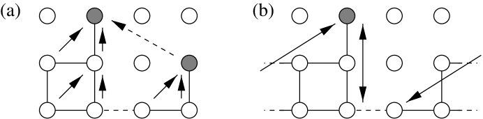
FIG. 1.: Two adjacent clusters in a bond percolation system. (a) The arrows represent pointers and the shaded sites are root nodes. (b) The difference in displacements (double-headed arrows) between the two sites and the root node of a cluster can be used as a criterion for detecting the onset of percolation.

FIG. 2.: Plots of the cluster wrapping probability functions $R_{L}(p)$ for $L=32$, $64$, $128$ and $256$ in the region of the percolation transition for percolation (a) along a specified axis, (b) along either axis, (c) along both axes, and (d) along one axis but not the other. Note that (d) has a vertical scale different from the other frames. The dotted lines denote the expected values of $p_{c}$ and $R_{\infty}(p_{c})$.

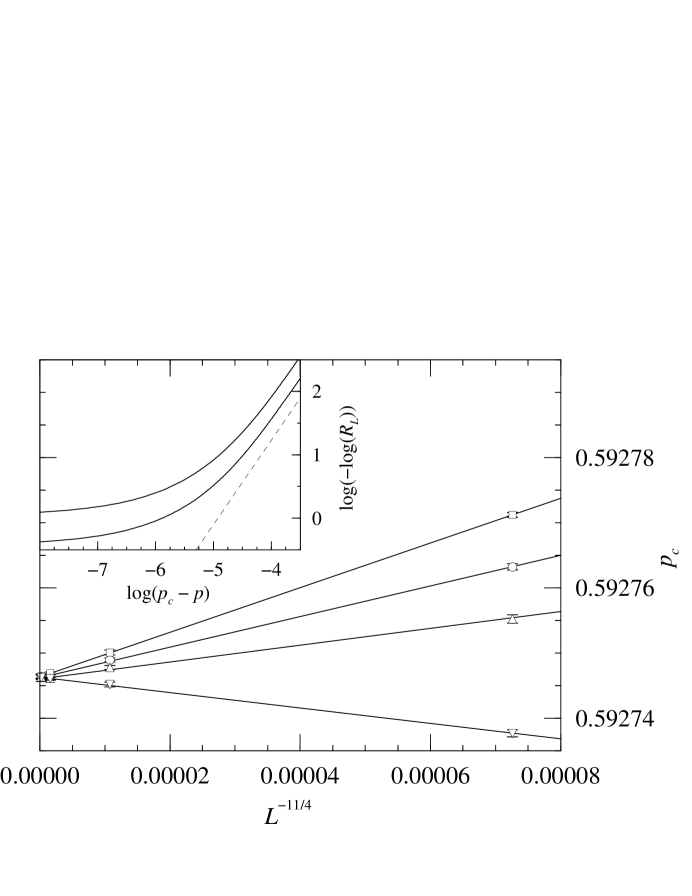
FIG. 3.: Finite-size scaling of the estimated value of $p_{c}$ for site percolation for $R_{L}^{(h)}$ (circles), $R_{L}^{(e)}$ (squares), $R_{L}^{(b)}$ (upward-pointing triangles), and $R_{L}^{(1)}$ (downward-pointing triangles). Inset: scaling plot of the wrapping probabilities $R_{L}^{(h)}$ (lower curve) and $R_{L}^{(b)}$ (upper curve). The dotted line indicates the slope of the expected $\frac{4}{3}$-power tail.

REFERENCES

- [1] D. Stauffer and A. Aharony, Introduction to Percolation Theory, 2nd edition, Taylor and Francis, London (1991).
- [2] L. de Arcangelis, S. Redner and A. Coniglio, Phys. Rev. B 31, 4725 (1985).
- [3] C. L. Henley, Phys. Rev. Lett. 71, 2741 (1993).
- [4] C. Moore and M. E. J. Newman, Phys. Rev. E 61, 5678 (2000).
- [5] B. Jovanovic, S. V. Buldyrev, S. Havlin and H. E. Stanley, Phys. Rev. E 50, 2403 (1994).
- [6] S. Solomon, G. Weisbuch, L. de Arcangelis, N. Jan and D. Stauffer, Physica A 277, 239–247 (2000).
- [7] J. Hoshen and R. Kopelman, Phys. Rev. B 14, 3438 (1976).
- [8] R. M. Ziff, P. T. Cummings and G. Stell, J. Phys. A 17, 3009 (1984).
- [9] P. Grassberger, J. Phys. A 25, 5475 (1992).
- [10] C.-K. Hu, Phys. Rev. B 46, 6592 (1992).
- [11] J.-P. Hovi and A. Aharony, Phys. Rev. E 53, 235 (1996).
- [12] An algorithm similar in some respects to ours is described in H. Gould and J. Tobochnik, An Introduction to Computer Simulation Methods, 2nd edition, Addison–Wesley, Reading, MA (1996), p. 444, but without the crucial components of (1) building the clusters at each step from those that existed before, (2) storing those clusters in a tree structure, and (3) using pointers to check efficiently for percolation at each step. Without these features the algorithm will run in time , giving it no advantage over the standard algorithms.
- [13] R. Sedgewick, Algorithms, 2nd edition, Addison-Wesley, Reading, Mass. (1988).
- [14] R. E. Tarjan, Journal of the ACM 22, 215 (1975).
- [15] J. Machta, Y. S. Choi, A. Lucke, T. Schweizer and L. M. Chayes, Phys. Rev. E 54, 1332 (1996).
- [16] H. T. Pinson, J. Stat. Phys. 75, 1167 (1994).
- [17] R. M. Ziff, C. D. Lorenz and P. Kleban, Physica A 266, 17 (1999).
- [18] R. M. Ziff, Phys. Rev. Lett. 69, 2670 (1992).
- [19] A figure of , which is compatible with the one obtained here, has been calculated by one of us in recent work using the hull-gradient method (R. M. Ziff, Int. J. Mod. Phys. C, in press).
- [20] L. Berlyand and J. Wehr, J. Phys. A 28, 7127 (1995).