The Role of Spin-Dependent Interface Scattering in Generating Current-Induced Torques in Magnetic Multilayers

I Introduction

Stacks of alternating ferromagnetic and nonmagnetic metal layers exhibit giant magnetoresistance (GMR), because their electrical resistance depends strongly on whether the moments of adjacent magnetic layers are parallel or antiparallel. This effect has allowed the development of new kinds of field-sensing and magnetic memory devices.[1] The cause of the GMR effect is that conduction electrons are scattered more strongly by a magnetic layer when their spins lie antiparallel to the layer’s magnetic moment than when their spins are parallel to the moment. Devices with moments in adjacent magnetic layers aligned antiparallel thus have a larger overall resistance than when the moments are aligned parallel, giving rise to GMR. This paper discusses the converse effect: just as the orientations of magnetic moments can affect the flow of electrons, then by Newton’s third law, a polarized electron current scattering from a magnetic layer can have a reciprocal effect on the moment of the layer. As proposed by Berger[2] and Slonczewski,[3] an electric current passing perpendicularly through a magnetic multilayer may exert a torque on the moments of the magnetic layers. This effect which is known as “spin transfer”,[4] may, at sufficiently high current densities, alter the magnetization state. It is a separate mechanism from the effects of current induced magnetic fields. Experimentally, spin-current-induced magnetic excitations such as spin-waves,[5, 6, 7, 8] and stable magnetic reversal,[7, 8] have been observed in multilayers, for current densities greater than $10^{7}A/cm^{2}$.

The spin-transfer effect offers the promise of new kinds of magnetic devices,[9] and serves as a new means to excite and to probe the dynamics of magnetic moments at the nanometer scale.[10] In order to controllably utilize these effects, however, it is necessary to achieve a better quantitative understanding of these current-induced torques. Slonczewski has presented a derivation of spin-transfer torques using a 1-D WKB approximation with spin-dependent potentials,[3] but his calculations only take into account electrons which are either completely transmitted or completely reflected by the magnetic layers. For real materials the degree to which an electron is transmitted through a magnetic/nonmagnetic interface depends sensitively on the matching of the band structures across the interface.[11, 12] It is the goal of this paper to incorporate such band structure information together with the effect of multiple reflections between the ferromagnetic layers, into a more quantitative theory of the torques generated by spin-transfer. This could be done using the formalism of Brataas et al,[13] which is based on kinetic equations for spin currents. Instead we choose to employ a modified Landauer-Büttiker formalism, in which we model the ferromagnetic layers as generalized spin-dependent scatterers. The calculations are carried out for a quasi-one dimensional geometry, for which we derive formulas for the torque generated on the magnetic layers when a current is applied to the system, for either ballistic or diffusive non-magnetic layers. The main difference between our approach and Ref. [13] is that in our case, scattering in the normal layer is phase coherent, whereas Ref. [13] assumes phase relaxation. However, in the case of a diffusive normal metal layer and for a large number of transverse modes, the two approaches would give the same answer.

The paper is organized as follows: in Section II, we present an intuitive picture (adapted from[2, 3]) of how spin-dependent scattering of a spin-polarized current produces a torque on a magnetic element. Section III is devoted to the introduction of the scattering matrix formalism for the spin-flux. This formalism is then used in Section IV to calculate the torque in a Ferromagnet-Normal-Ferromagnet (FNF) system where the normal part is disordered (diffusive). Section V contain a discussion of the results. Details of our calculation are presented in Appendix A. In appendix B, we derive the torque for an FNF system where transport in the normal layer is ballistic, rather than diffusive.

II Physical Idea

In this section we will present a simple intuitive picture of the physics behind the spin-transfer effect. The connection between current-induced spin-transfer torques and the spin-dependent scattering that occurs when electrons pass through a magnetic/nonmagnetic interface can be illustrated most simply by considering the case of a spin-polarized current incident perpendicularly on a single thin ferromagnetic layer F, as shown in Figure 1. The layer lies in the $y-z$ plane, with its magnetic moment uniformly pointed in the $+z$ direction, and we assume that the current is spin-polarized in the $z-x$ plane at an angle $\theta$ to the layer moments. The incoming electrons can therefore be considered as a coherent linear superposition of basis states with spin in the +z direction (amplitude $\cos(\theta/2)$) and -z direction (amplitude $\sin(\theta/2)$). For this initial discussion we will assume that the layer is a perfect spin-filter, so that spins aligned with the layer moments are completely transmitted through the layer, while spins aligned antiparallel to the layer moment are completely reflected. For incident spins polarized at an angle $\theta$, the average outgoing current will have the relative weights $\cos^{2}(\theta/2)$ polarized in the $+z$ direction and transmitted to the right and $\sin^{2}(\theta/2)$ polarized in the $-z$ direction and reflected to the left. Consequently, both of the outgoing electron spin fluxes (transmitted and reflected) lie along the $z$ axis, while the incoming (incident) electron flux has a component perpendicular to the magnetization, along the $x$ axis, with magnitude proportional to $\sin\theta$. This $x$-component of angular momentum must be absorbed by the layer in the process of filtering the spins. Because the spin-filtering is ultimately governed by the $s-d$ exchange interaction between the conduction electrons and the magnetic moments of the layer, the angular momentum is imparted to the layer moments and produces a torque on them. This exchange torque,[14] which is proportional to the electron current through the layer and to $\sin\theta$, is in the direction to align the moments with the polarization of the incident spin current.

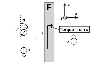
FIG. 1.: Schematic of exchange torque generated by spin-filtering. Spin-polarized electrons are incident perpendicularly on a thin ideal ferromagnetic layer. Spin-filtering removes the component of spin angular momentum perpendicular to the layer moments from the current; this is absorbed by the moments themselves, generating an effective torque on the layer moments.

The symmetry of this model precludes any generation of torque from the spin-filtering of a current of unpolarized electrons. To generate the effect, then, a second ferromagnetic layer is needed to first spin-polarize the current, see Fig. 2. In that case, spin angular momentum is transferred from one layer to the flowing electrons and then from the electrons to the second layer. However, the torques on the two layers are not equal and opposite, as spin angular momentum carried by the electrons can also flow away from the layers to infinity, see Fig. 2.

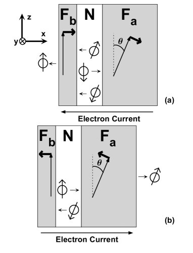
FIG. 2.: Qualitative picture of asymmetry of spin-transfer torque with respect to current bias in a FNF junction. For left-going electrons (2a), initially polarized by a magnetic layer F_a, the moments of layer F_b experience a torque so as to align them with layer F_a. The electron current reflected from layer F_b, in turn, exerts a torque on layer F_a so as to antialign it with the moment of layer F_b. Subsequent reflections between the layers reduce but do not eliminate this torque. If the current is reversed $(2b)$ the overall sign of the torque is reversed, encouraging the moment of layer F_b to align antiparallel with layer F_a.

The presence of this second layer has the additional effect of allowing for multiple scattering of the electrons between the two layers, which gives rise to an explicit asymmetry of the torque with respect to current direction. This asymmetry is an important signature which can be used to distinguish spin-transfer-induced torques from the torques produced by current-generated magnetic fields. To see how the asymmetry arises, consider the ferromagnet–normal-metal–ferromagnet (FNF) junction shown in Figure 2. It consists of two ferromagnetic layers, F_a and F_b, with moments pointing in directions $\hat{m}_{a}$ and $\hat{m}_{b}$, separated by a normal metal spacer N. Normal metal leads on either side of the trilayer inject an initially unpolarized current into the system. When the current enters the sample from the left (Fig. 2a), electrons transmitted through F_a will be polarized along $\hat{m}_{a}$. As long as the normal metal spacer is smaller than the spin-diffusion length (100 nm for Cu), this current will remain spin-polarized when it impinges on F_b and will exert a torque on the moment of F_b in a direction so as to align $\hat{m}_{b}$ with $\hat{m}_{a}$. Repeating the argument for F_b, we find that the spin of the electrons reflected from layer F_b is aligned antiparallel to $\hat{m}_{b}$, and, hence in turn, exerts a torque on the moment of F_a trying to align $\hat{m}_{a}$ antiparallel with $\hat{m}_{b}$. (Subsequent multiple reflections of electrons between F_a and F_b can serve to reduce the magnitudes of the initial torques, but they do not eliminate or reverse them, as the electron flux is reduced upon each reflection.) When the current is injected from the right, the directions of the torques are reversed: Now the flow of electrons exerts a torque on F_a trying to align its moment parallel with $\hat{m}_{b}$, while it exerts a torque on F_b so as to force the moment in layer F_b antiparallel with $\hat{m}_{a}$.

In the remainder of the paper, we assume that $\hat{m}_{b}$ points in the $+z$ direction, while $\hat{m}_{a}$ differs by a small angle $\theta$ in the $x-z$ plane. (For thin films, demagnetizing forces will in general cause the $y-z$ plane to be preferred, but this produces no change in our argument. We present the case that is easier to draw.) The overall effect of a left-going flow of electrons then, is to exert a torque $\vec{\tau}_{b}$ on F_b in the $+x$ direction. If we reverse the current, so that electrons pass through F_b first (Fig. 2b), the torque on F_b is only exerted by the electrons after they have been reflected from F_a. As seen before, the electrons reflected from F_a have polarizations opposite to $\hat{m}_{a}$, so that the torque on F_b is in the $-x$ direction.

In Refs. [3] and [7], the layer F_a was taken to be much thicker than F_b, so that intralayer exchange and anisotropy forces will hold the orientation of $\hat{m}_{a}$ fixed. In that case, one is only interested in the torque on F_b, which serves to align $\hat{m}_{b}$ either parallel or antiparallel with the fixed moment $\hat{m}_{a}$ depending on the current direction. This asymmetric current response has been employed in both a point-contact geometry[7] and in a thin-film pillar geometry [8] to switch the moments in FNF trilayers from a parallel to an antiparallel configuration by a current pulse in one direction, and then from antiparallel to parallel by a reversed current. For weakly-interacting layers, either orientation can be stable in the absence of an applied current, so that the resistance versus current characteristic is hysteretic, and the devices can function as simple current-controlled memory elements.

III Spin flux and torque in the scattering approach

Treating the ferromagnetic layers as perfect spin filters provides important qualitative insights into spin-transfer, but for a complete qualitative and quantitative picture, a more general approach is required. In this section, we introduce a scattering matrix description of the FNF junction which allows us to deal with non-ideal (magnetic and non-magnetic) layers. Our goal is to relate the torque $\vec{\tau}_{b}$ exerted on layer F_b by an unpolarized incident electron beam to the scattering properties of the layers. Although we shall restrict our formulas to the FNF junction (see Fig. 3), our method is applicable for an arbitrary array of magnetic-nonmagnetic layers.

We first introduce the spin flux $\vec{J}$ in the $x$-direction (the direction of current flow):

$$\vec{J}(x)=\frac{\hbar^{2}}{2m}{\rm Im}\int dydz\left[\phi^{\dagger}(x)\vec{\sigma}\frac{\partial}{\partial x}\phi(x)\right]$$ (1)

where $\phi(x)$ is a spinor wavefunction and $\vec{\sigma}$ the vector of Pauli matrices,

$$\phi(x)=\left(\begin{array}[]{c}\phi_{\uparrow}(x)\\ \phi_{\downarrow}(x)\end{array}\right),\ \vec{\sigma}=\left(\begin{array}[]{c}\sigma_{x}\\ \sigma_{y}\\ \sigma_{z}\end{array}\right).$$

Note that although Eq.(1) bears close formal analogy to the particle current, no local equation of conservation can be written for the spin flux, since in general, the Hamiltonian does not conserve spin. Specifically, the magnetic layers can act as sources and sinks of spin flux, so that the spin flux on different sides of a F layer can be different.

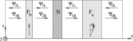
FIG. 3.: Schematic of the setup used for the definition of the scattering matrices of the F and N layers. The two layers F_a and F_b are ferromagnetic layers whose magnetic moment is oriented as shown in the bottom of the figure. The layer N is a nonmagnetic metal spacer. Amplitude of left and right moving propagating waves are defined in fictitious ideal leads $0$, $1$, $2$ and $3$ between the layers and between the layers and the reservoirs.

A Definition of the scattering matrices

Fig. 3 shows the FNF junction where (fictitious) perfect leads (labeled $0$, $1$, $2$ and $3$) have been added in between the layers F and N and between the F layers and the electron reservoirs on either side of the sample. The introduction of these leads allows for a description of the system using scattering matrices. In the perfect leads, the transverse degree of freedom are quantized, giving $N$ propagating modes at the Fermi level, where $N\sim A/\lambda_{F}^{2}$ $A$ being the cross section area of the junction and $\lambda_{F}$ the Fermi wave length. Expanding the electronic wave function in these modes, we can describe the system in terms of the projection $\Psi_{i,L/R}$ of the wave function onto the left (right) going modes in region $i$. The $\Psi_{i,L/R}$ are $2N$-component vectors, counting the $N$ transverse modes and spin. The amplitudes of the wave function in two neighboring ideal leads are connected through the scattering matrices $S_{b}$, $S_{a}$ and $S_{\rm N}$, that relate amplitudes of outgoing modes and incoming modes at the layer (see for example Ref. [15] for a review of the scattering matrix approach),

$$\left(\begin{array}[]{c}\Psi_{3L}\\ \Psi_{2R}\end{array}\right) = S_{b}\left(\begin{array}[]{c}\Psi_{3R}\\ \Psi_{2L}\end{array}\right),$$ (7)

$$\left(\begin{array}[]{c}\Psi_{1L}\\ \Psi_{0R}\end{array}\right) = S_{a}\left(\begin{array}[]{c}\Psi_{1R}\\ \Psi_{0L}\end{array}\right),$$ (12)

$$\left(\begin{array}[]{c}\Psi_{2L}\\ \Psi_{1R}\end{array}\right) = S_{\rm N}\left(\begin{array}[]{c}\Psi_{2R}\\ \Psi_{1L}\end{array}\right).$$ (17)

The scattering matrices $S_{b}$, $S_{a}$ and $S_{\rm N}$ are $4N\times 4N$ unitary matrices. We decompose $S_{b}$ into $2N\times 2N$ reflection and transmission matrices,

$$S_{b}=\left(\begin{array}[]{cc}r_{b}&t^{\prime}_{b}\\ t_{b}&r^{\prime}_{b}\end{array}\right),$$ (18)

with similar decompositions of $S_{a}$ and $S_{\rm N}$. Normalization is done in such a way that each mode carries unit current. Due to the spin degree of freedom, the reflection and transmission matrices can be written in terms of four $N\times N$ blocks:

$$r_{b}=\left(\begin{array}[]{cc}r_{b\uparrow\uparrow}&r_{b\uparrow\downarrow}\\ r_{b\downarrow\uparrow}&r_{b\downarrow\downarrow}\end{array}\right),$$ (19)

where the subscripts $\uparrow,\downarrow$ refer to spin up and down in the $z$-axis basis.

The scattering matrix of the magnetic layers depends on the angle $\theta$ the moments may make with the z-axis. The matrix $S_{a}(\theta)$ is related to $S_{a}(\theta=0)$ through a rotation in spin space:

$$r_{a}(\theta) = R_{\theta}\ r_{a}(0)\ R_{-\theta},\ \ r^{\prime}_{a}(\theta)=R_{\theta}\ r^{\prime}_{a}(0)\ R_{-\theta},$$ (20)

$$t_{a}(\theta) = R_{\theta}\ t_{a}(0)\ R_{-\theta},\ \ t^{\prime}_{a}(\theta)=R_{\theta}\ t^{\prime}_{a}(0)\ R_{-\theta}$$ (21)

where

$$R_{\theta}=\left(\begin{array}[]{cc}\cos\frac{\theta}{2}&-\sin\frac{\theta}{2}\\ \sin\frac{\theta}{2}&\cos\frac{\theta}{2}\end{array}\right)\otimes 1_{N}.$$ (22)

The non-magnetic metallic layer will not affect the spin states, i.e., $r_{\rm N\uparrow\downarrow}=r_{\rm N\downarrow\uparrow}=0$ and $r_{\rm N\uparrow\uparrow}=r_{\rm N\downarrow\downarrow}$.

We need to keep track of the amplitudes within the system in order to calculate the net spin flux deposited into each magnetic layer. Therefore, we define $2N\times 2N$ matrices $\Gamma_{i}^{L/R}$ and $\Lambda_{i}^{L/R}$ ($i=0,1,2,3$) so that we may express all the $\Psi_{i,L/R}$ as a function of the amplitudes incident from the two electrodes (regions 0 and 3):

$$\left(\begin{array}[]{c}\Psi_{iL}\\ \Psi_{iR}\end{array}\right)=\left(\begin{array}[]{cc}\Gamma_{iL}&\Lambda_{iL}\\ \Gamma_{iR}&\Lambda_{iR}\end{array}\right)\left(\begin{array}[]{c}\Psi_{0L}\\ \Psi_{3R}\end{array}\right)$$ (23)

with the convention that $\Gamma_{0L}=\Lambda_{3R}=1$ and $\Gamma_{3R}=\Lambda_{0L}=0$. In order to calculate the torque exercised on layer F_b for a current entering from the left, we need the matrix, $\Gamma_{2L}$. To simplify the notations in the rest of the paper, we write

$$\Omega\equiv\Gamma_{2L}.$$ (24)

The matrix $\Omega$ relates $\Psi_{2L}$ to the incoming amplitudes $\Psi_{0L}$ coming from the right. To calculate it, we put $\Psi_{3R}=0$, then, using Eq.(III A), we get the equations:

$$\Psi_{1L} = t^{\prime}_{a}\Psi_{0L}+r_{a}\Psi_{1R},$$ (25)

$$\Psi_{1R} = t_{n}\Psi_{2R}+r^{\prime}_{n}\Psi_{1L},$$ (26)

$$\Psi_{2L} = r_{n}\Psi_{2R}+t^{\prime}_{n}\Psi_{1L},$$ (27)

$$\Psi_{2R} = r^{\prime}_{b}\Psi_{2L},$$ (28)

$$\Psi_{3L} = t^{\prime}_{b}\Psi_{2L},$$ (29)

from which we obtain:

$$\Omega=\frac{1}{1-r_{n}r^{\prime}_{b}}t^{\prime}_{n}\frac{1}{1-r_{a}t_{n}r^{\prime}_{b}\frac{1}{1-r_{n}r^{\prime}_{b}}t^{\prime}_{n}-r_{a}r^{\prime}_{n}}t^{\prime}_{a}.$$ (30)

B Spin flux response

Let us now connect our system to two unpolarized electron reservoirs on its two sides, as shown in Fig. 4. In equilibrium, the modes in the reservoirs are filled up to the fermi level $\epsilon_{F}$. We want to calculate the spin current that is generated when the chemical potential in the left (right) reservoir is slightly increased by $\delta\mu_{3}$ ($\delta\mu_{0}$). The spin current $\vec{J_{i}}$ is the difference of the left going and right going contributions. For each of the region $i=0,1,2,3$, we find from Eq.(1) and Eq.(23):

$$\frac{\partial\vec{J_{i}}}{\partial\mu_{3}}=\frac{1}{4\pi}{\rm Re}\left[{\rm Tr}\vec{\sigma}\Gamma_{iR}\Gamma_{iR}^{\dagger}-{\rm Tr}\vec{\sigma}\Gamma_{iL}\Gamma_{iL}^{\dagger}\right],$$ (31)

and

$$\frac{\partial\vec{J_{i}}}{\partial\mu_{0}}=\frac{1}{4\pi}{\rm Re}\left[{\rm Tr}\vec{\sigma}\Lambda_{iR}\Lambda_{iR}^{\dagger}-{\rm Tr}\vec{\sigma}\Lambda_{iL}\Lambda_{iL}^{\dagger}\right].$$ (32)

Derivation of Eq.(31) and Eq.(32) proceeds analogously to the derivation of the Landauer formula for the conductance.[16]

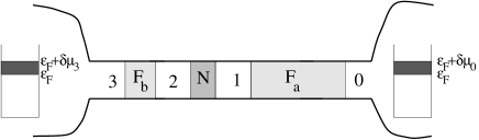
FIG. 4.: The FNF junction is connected to two reservoirs.

C Torque exercised on layer F_b

If the spin flux on both sides of F_b (region 2 and 3) is different, then angular momentum has been deposited in the layer F_b. This creates a torque $\vec{\tau_{b}}$ on the moment of the ferromagnet,

$$\vec{\tau_{b}}=\vec{J}_{3}-\vec{J}_{2}.$$ (33)

Setting $\delta\mu_{0}=-eV_{0}$, we have:

$$\frac{\partial\vec{\tau}_{b}}{\partial V_{0}}=-\frac{e}{4\pi}{\rm Re\ \ Tr}_{2N}\left[\vec{\Sigma}\Omega\Omega^{\dagger}\right],$$ (34)

with

$$\vec{\Sigma}=\vec{\sigma}-t^{\prime^{\prime}\dagger}_{b}\vec{\sigma}t^{\prime}_{b}-r^{\prime\dagger}_{b}\vec{\sigma}r^{\prime}_{b}.$$ (35)

This equation can be simplified further if the spin-transfer effect is due entirely to spin-filtering (as argued by Slonczewski[3]) as opposed to spin-flip scattering of electrons from the magnetic layers. That is, if we assume that $r_{b\uparrow\downarrow}=r_{b\downarrow\uparrow}=r_{a\uparrow\downarrow}(\theta=0)=r_{a\downarrow\uparrow}(\theta=0)=0$, then:

$$\frac{\partial\tau_{b}^{x}}{\partial V_{0}}=-\frac{e}{2\pi}{\rm Re\ \ Tr}_{N}\left[(\Omega_{\uparrow\uparrow}\Omega_{\downarrow\uparrow}^{\dagger}+\Omega_{\uparrow\downarrow}\Omega_{\downarrow\downarrow}^{\dagger})\right.$$

$$\left.(1-r^{\prime}_{b\uparrow\uparrow}r^{\prime\dagger}_{b\downarrow\downarrow}-t^{\prime}_{b\uparrow\uparrow}t^{\prime\dagger}_{b\downarrow\downarrow})\right]$$ (36)

We will comment briefly in the conclusion of this paper about the physical implications of including the off-diagonal spin-flip terms, as well.

We note that, as there is no spin flux conservation in this system, $\partial\vec{J_{i}}/\partial\mu_{3}$ can be different from $-\partial\vec{J_{i}}/\partial\mu_{0}$ and, hence, there can be a non zero spin flux even when the chemical potentials are identical in the two reservoirs. The existence of a zero-bias spin-flux and the resulting torques reflect the well-known itinerant-electron-mediated exchange interaction (a.k.a. the RKKY interaction) between two ferromagnetic films separated by a normal-metal spacer. This interaction can in fact be understood within a scattering framework.[17, 18, 19, 20] The zero-bias torque has to be added to the finite-bias contribution (given by Eq.(36)). Since the former is typically a factor $N^{-1}$ smaller and vanishes upon ensemble averaging (see section IV and Ref.[15]), we henceforth neglect the zero-bias contribution to the torque and restrict our attention to the bias induced torque, for which we have

$$\frac{\partial\vec{\tau}_{b}}{\partial V_{0}}=-\frac{\partial\vec{\tau}_{b}}{\partial V_{3}}$$

up to a correction of order $N^{-1}$.

IV Averaging over the normal layer

Via Eq.(36), the torque on the moments of the ferromagnetic layers F_a and F_b not only depends on the scattering matrices $S_{a}$ and $S_{b}$ of these layers, but also of the scattering matrix $S_{\rm N}$ of the normal metal layer in between. If the normal layer is disordered, $\vec{\tau}_{a}$ and $\vec{\tau}_{b}$ depend on the location of the impurities; if N is ballistic the torque depend sensitively on the electronic phase shift accumulated in N. In general, sample to sample fluctuations of the torque will be a factor $N^{-1}$ smaller than the average.[15] Hence, if $N$ is large ($N>10^{3}$ in the experiments of Ref.[7]), the torque is well characterized by its average. In this section, we average over $S_{\rm N}$ for the case where N is disordered. The case of ballistic N is addressed in appendix B. After averaging, the zero-bias spin transfer current, corresponding to the RKKY interaction described above, vanishes, and only the torque caused by the electron current remains. Because all effects of quantum interference in the N layer will disappear in the process of averaging (to leading order in the number of modes $N$), the results we derive are unchanged if the reflection and transmission matrices include processes in which the energy of the electron changes during scattering,[13] in addition to the elastic proceses normally considered in scattering matrix calculations.

A Averaged torque

The scattering matrix of the normal layer can be written using the standard polar decomposition:[21]

$$S_{n}=\left(\begin{array}[]{cc}U&0\\ 0&V^{\prime}\end{array}\right)\left(\begin{array}[]{cc}\sqrt{1-T}&i\sqrt{T}\\ i\sqrt{T}&\sqrt{1-T}\end{array}\right)\left(\begin{array}[]{cc}U^{\prime}&0\\ 0&V\end{array}\right)$$ (37)

where $U,V,U^{\prime}$ and $V^{\prime}$ are $2N\times 2N$ unitary matrices and T is a diagonal matrix containing the eigenvalues of $t_{n}t_{n}^{\dagger}$. Since $S_{\rm N}$ is diagonal in spin space, we find that $U$, $U^{\prime}$, $V$ and $V^{\prime}$ are block diagonal.

$$U=\left(\begin{array}[]{cc}u&0\\ 0&u\end{array}\right),\ \ U^{\prime}=\left(\begin{array}[]{cc}u^{\prime}&0\\ 0&u^{\prime}\end{array}\right),$$ (38)

and similar definitions for $v$ and $v^{\prime}$. In the isotropic approximation[15, 21], the $N\times N$ unitary matrices $u,u^{\prime},v$ and $v^{\prime}$ are uniformly distributed in the group $U(N)$. (The outer matrices in Eq.(37) thus mix the modes in a ergodic way while the central matrix contains the transmission properties of the layer, which determine the average conductance of N.)

We want to average Eq.(36) over both the unitary matrices and $T$. A diagrammatic technique for such averages has already been developed in Ref.[22] and can be used to calculate $\langle\partial\vec{\tau}_{b}/\partial V_{0}\rangle$ in leading order in $1/N$. It is a general property of such averages that the fluctuations are a factor of order $N$ smaller than the average. This justifies our statement above, that the ensemble averaged torque is sufficient to characterize the torque exerted on a single sample. Details of the calculation are presented in Appendix A.

The resulting expression for $\langle\partial\vec{\tau}_{b}/\partial V_{0}\rangle$ can be written in a form very similar to the one for Eq.(36) if one uses a notation that involves $4\times 4$ matrices. To be specific, to each $2N\times 2N$ matrix $A$ appearing in Eq.(36) and Eq.(30), we assign a $4\times 4$ matrix $\hat{A}$ as,

$$\hat{A}=\frac{1}{N}{\rm Tr}_{N}\left[A\otimes A^{\dagger}\right],$$ (39)

where ${\rm Tr}_{N}$ means that the trace has been taken in each the $N\times N$ blocks, or in extenso:

$$\hat{A}=\frac{1}{N}{\rm Tr}_{N}\left(\begin{array}[]{cccc}A_{\uparrow\uparrow}A_{\uparrow\uparrow}^{\dagger}&A_{\uparrow\uparrow}A_{\uparrow\downarrow}^{\dagger}&A_{\uparrow\downarrow}A_{\uparrow\uparrow}^{\dagger}&A_{\uparrow\downarrow}A_{\uparrow\downarrow}^{\dagger}\\ A_{\uparrow\uparrow}A_{\downarrow\uparrow}^{\dagger}&A_{\uparrow\uparrow}A_{\downarrow\downarrow}^{\dagger}&A_{\uparrow\downarrow}A_{\downarrow\uparrow}^{\dagger}&A_{\uparrow\downarrow}A_{\downarrow\downarrow}^{\dagger}\\ A_{\downarrow\uparrow}A_{\uparrow\uparrow}^{\dagger}&A_{\downarrow\uparrow}A_{\uparrow\downarrow}^{\dagger}&A_{\downarrow\downarrow}A_{\uparrow\uparrow}^{\dagger}&A_{\downarrow\downarrow}A_{\uparrow\downarrow}^{\dagger}\\ A_{\downarrow\uparrow}A_{\downarrow\uparrow}^{\dagger}&A_{\downarrow\uparrow}A_{\downarrow\downarrow}^{\dagger}&A_{\downarrow\downarrow}A_{\downarrow\uparrow}^{\dagger}&A_{\downarrow\downarrow}A_{\downarrow\downarrow}^{\dagger}\end{array}\right).$$ (40)

We also define $\hat{\vec{\Sigma}}$ by,

$$\hat{\vec{\Sigma}}={\rm Tr}_{N}\left(\begin{array}[]{cccc}\vec{\Sigma}_{\uparrow\uparrow}&\vec{\Sigma}_{\downarrow\uparrow}&\vec{\Sigma}_{\uparrow\downarrow}&\vec{\Sigma}_{\downarrow\downarrow}\\ 0&0&0&0\\ 0&0&0&0\\ \vec{\Sigma}_{\uparrow\uparrow}&\vec{\Sigma}_{\downarrow\uparrow}&\vec{\Sigma}_{\uparrow\downarrow}&\vec{\Sigma}_{\downarrow\downarrow}\\ \end{array}\right).$$ (41)

The average over the transmission eigenvalues $T$ follows if we note that the average of a function is the function of the average, to leading order in $1/N$.[15] Thus the average over $T$ amounts to the replacement

$$\hat{t}_{n}=\frac{g_{\rm N}}{N}\openone_{4}{\rm\ \ and\ \ }\hat{r}_{n}=\left(1-\frac{g_{\rm N}}{N}\right)\openone_{4},$$ (42)

where $g_{\rm N}$ is the conductance of the normal layer and $\openone_{4}$ is the $4\times 4$ unit matrix. Using these “hat” matrices, the result has now the simple form:

$$\langle\frac{\partial\vec{\tau}_{b}}{\partial V_{0}}\rangle=-\frac{e}{4\pi}{\rm Re\ \ Tr}_{4}\left[\hat{\vec{\Sigma}}\hat{\Omega}\right],$$ (43)

where (compare to Eq.(30)),

$$\hat{\Omega}=\frac{1}{1-\hat{r}_{n}\hat{r}^{\prime}_{b}}\hat{t}^{\prime}_{n}\frac{1}{1-\hat{r}_{a}\hat{t}_{n}\hat{r}^{\prime}_{b}\frac{1}{1-\hat{r}_{n}\hat{r}^{\prime}_{b}}\hat{t}^{\prime}_{n}-\hat{r}_{a}\hat{r}^{\prime}_{n}}\hat{t}^{\prime}_{a}.$$ (44)

Equation (43) is the main result of this paper. In the absence of spin-flip scattering, it reduces to

$$\langle\frac{\partial\tau_{b}^{x}}{\partial V_{0}}\rangle = -\frac{e}{2\pi}{\rm Re}\left[(\hat{\Omega}_{3,1}+\hat{\Omega}_{3,4})\right.$$ (45)

$$\times \left.{\rm Tr}_{N}(1-r^{\prime}_{b\uparrow\uparrow}r^{\prime\dagger}_{b\downarrow\downarrow}-t^{\prime}_{b\uparrow\uparrow}t^{\prime\dagger}_{b\downarrow\downarrow})\right].$$ (46)

The same formalism can be used to calculate the conductance $g$ of the system using the Landauer formula. One gets:

$$\langle g\rangle=\frac{Ne^{2}}{h}\left[\hat{t^{\prime}}_{1,1}+\hat{t^{\prime}}_{1,4}+\hat{t^{\prime}}_{4,1}+\hat{t^{\prime}}_{4,4}\right],$$ (47)

$t^{\prime}$ being the total transmission matrix:

$$t^{\prime}=t^{\prime}_{b}\ \Omega.$$ (48)

We would like to note that, while our theory started from a fully phase coherent description of the FNF trilayer, including the full $4N\times 4N$ scattering matrices of the FN interfaces, the final result can be formulated in term of $2\times 4$ parameters, represented by the matrices $\hat{r}_{a}$ and $\hat{r}^{\prime}_{b}$ ( $2\times 16$ parameters in case of spin-flip scattering). Such a reduction of the number of degrees of freedom was also found by Brataas et al.,[13] although their starting point is an hybrid ferromagnetic-normal metal circuit with incoherent nodes. This confirms the statement at the beginning of this section, that for a diffusive normal-metal spacer all effects of quantum interferences are washed out.[15] The difference between our approach and the one of Ref. [13] is important in the case of the ballistic normal layer, see Appendix B.

B Symmetries

Before we proceed with a further analysis of Eq.(43), we identify the different symmetries of the torque. Due to the conservation of current, the total torque deposited on the full system is anti-symmetric with respect to current direction:

$$\frac{\partial\vec{\tau}_{b}}{\partial V_{0}}+\frac{\partial\vec{\tau}_{a}}{\partial V_{0}}=-\left[\frac{\partial\vec{\tau}_{b}}{\partial V_{3}}+\frac{\partial\vec{\tau}_{a}}{\partial V_{3}}\right].$$ (49)

Eq.(49) holds before averaging. But, as pointed out in section III, equality for each of the torques $\vec{\tau}_{a}$ and $\vec{\tau}_{b}$ separately holds only after averaging,

$$\langle\frac{\partial\vec{\tau}_{b}}{\partial V_{0}}\rangle=-\langle\frac{\partial\vec{\tau}_{b}}{\partial V_{3}}\rangle;$$ (50)

sample to sample fluctuations of $\partial\vec{\tau}_{b}/\partial V_{0}$ and $-\partial\vec{\tau}_{b}/\partial V_{3}$ of relative order $1/N$ are in general different. Thus, for $N\gg 1$, our calculation can be used to compute the linear response of the torque to a small bias voltage:

$$\vec{\tau}_{b}=\langle\frac{\partial\vec{\tau}_{b}}{\partial V_{0}}\rangle(V_{0}-V_{3}).$$ (51)

In our geometry, where F_a and F_b are in $x-z$ plane, the only non-zero component of the torque is $\tau_{b}^{x}$. The torque vanishes when the moments are completely aligned or antialigned (all the matrices are diagonal in spin space and therefore no x-component of the spin can be found). Around these two limits, the torque is symmetric in respect to the angle ($\theta\rightarrow-\theta$ and $\pi-\theta\rightarrow\pi+\theta$). There is no symmetry between $\theta$ and $\pi-\theta$. In addition, the two layers are not equivalent and exchanging the scattering matrices of F_a and F_b also changes the torque.

C Discussion of some limiting cases

Eq.(43) can be simplified in some particular cases. Let us start with the simplest case of ideal spin filters, so that majority (minority) spins are totally transmitted (reflected) by either layer. Equation (43) then reduces to

$$\langle\frac{\partial\tau_{b}^{x}}{\partial V_{0}}\rangle=-\frac{e}{4\pi}\frac{g_{\rm N}\sin\theta}{3+\cos\theta}=-\frac{h}{4\pi e}\langle g\rangle\frac{\tan\theta/2}{2},$$ (52)

where $\langle g\rangle$ is the average magnetoconductance, cf Eq.(47),

$$\langle g\rangle=\frac{e^{2}}{h}g_{\rm N}\frac{4\cos^{2}\theta/2}{3+\cos\theta}.$$ (53)

Equation (52) reproduces a result of Slonczewski.[3] As expected, for left-going electrons ($V_{0}<0$) the torque is positive, so it acts to align the moments of the two magnetic layers, see section II.

Let us now consider the case of weak $s-d$ exchange coupling, i.e., when the scattering coefficients depend only weakly on spin. We continue to assume that no spin-flip scattering occurs in the ferromagnetic layers. We define $g_{a}$ and $g_{b}$ as the average conductance per spin of the two layers (in unit of $e^{2}/h$). Then, the conductance of F_a alone is $g_{a}+\delta g_{a}$ and $g_{a}-\delta g_{a}$ for respectively the majority and minority spins, which defines the spin scattering asymmetry $\delta g_{a}$. In that case, we get to lowest nontrivial order in $\delta g_{a}$ and $\delta g_{b}$:

$$\langle g\rangle = \frac{2e^{2}}{h}\left(\frac{g_{\rm N}g_{a}g_{b}}{g_{a}g_{b}+g_{\rm N}(g_{a}+g_{b}-2\frac{g_{a}g_{b}}{N})}\right.$$ (54)

$$+ \left.\frac{g_{\rm N}^{2}\delta g_{a}\delta g_{b}\cos\theta}{(\frac{g_{a}g_{b}}{N}+g_{\rm N}(g_{a}+g_{b}-2\frac{g_{a}g_{b}}{N}))^{3}}\right)$$ (55)

and

$$\langle\frac{\partial\tau_{b}^{x}}{\partial V_{0}}\rangle=-\frac{e}{2\pi}\frac{g_{\rm N}^{2}\delta g_{a}\ \delta g_{b}^{2}\sin\theta}{2(1-\frac{g_{b}}{N})(g_{a}g_{b}+g_{\rm N}(g_{a}+g_{b}-2\frac{g_{a}g_{b}}{N}))^{2}}.$$ (56)

This last formula shows that:

(i) The torque is not symmetric with respect to interchanging the layer F_a and F_b, in contrast to the conductance. If one changes $\delta g_{a}$ to $-\delta g_{a}$, the sign of the torque is reversed. However, $\langle\partial\tau_{b}^{x}/\partial V_{0}\rangle\propto\delta g_{b}^{2}$, so if one changes $\delta g_{b}$ to $-\delta g_{b}$, the sign of the torque is unchanged. The sign of the torque on a ferromagnetic layer therefore depends on whether the other layer is a positive or negative polarizer, but not on the sign of filtering for the layer experiencing the torque. We have verified that this is true also in the general case. This point explains why the two layers can not be treated on an equal footing.

(ii) We see that $g_{\rm N}$ appears through its square. Indeed, in order for some spin to be deposited in the layer F_b, some left going electrons have to be reflected by F_b and exit the system from the right hand side. Therefore these electrons cross the normal layer at least twice and this leads to the factor $g_{\rm N}^{2}$. On the other hand the conductance is linear in $g_{\rm N}$. Therefore in order to maximize the torque deposited per current, one has to use the cleanest possible normal metal spacer. (This statement is true in this limit of weak filtering, but not in general, see section V.) Note that in the previous case (perfect spin-filtering) the torque is proportional to $g_{\rm N}$ instead of the expected $g_{\rm N}^{2}$. Indeed, in that case, once the electron has been reflected by the layer F_b, it cannot go through F_b which works as a perfect wall for it. Therefore current conservation implies that it goes out of the system through the right. For $g_{\rm N}\ll N$, the torque is actually proportional to $g_{\rm N}^{2}$ for arbitrary spin asymmetry (except perfect filtering), and one gets:

$$\langle\frac{\partial\tau_{b}^{x}}{\partial V_{0}}\rangle\propto g_{\rm N}^{2}\sin\theta,\ \ \ g_{\rm N}\ll N,$$ (57)

the factor of proportionality being a complicated function of the transmission probabilities of the layers.

V Application to current-driven switching of magnetic domains

In this section, we consider the general solution Eq.(43) for the spin-transfer torque. We first address strongly polarizing systems and then calculate torques for scattering parameters more appropriate for the transition metal trilayers that can be studied experimentally. As the trilayer devices are primarily current-driven, we calculate the torque per unit of current $I$,

$$\frac{\tau_{b}^{x}}{I}=\langle\frac{1}{g}\frac{\partial\tau_{x}}{\partial V_{0}}\rangle.$$

The torque is measured in units of $\frac{h}{2\pi e}$.

FIG. 5.: Torque per unit current for the case where F_b is a nearly perfect polarizer ($|t_{b\uparrow}|^{2}=0.999$, $|t_{b\downarrow}|^{2}=0.001$) and F_a is not ($|t_{a\uparrow}|^{2}=0.3$ $|t_{a\downarrow}|^{2}=0.01$). (solid line). The dashed line shows the case of perfect polarizers, see Eq.(52). Torque in measured in unit of $\frac{h}{2\pi e}$.

Eq. (52) of the previous section gives the torque per unit current for the case that both layers F_a and F_b are perfect polarizers. The main feature of this system is that the $\theta$ dependence of the torque is not of a simple $\sin\theta$ form, and that the torque per unit current diverges at $\theta=0$. In Fig. 5, we look at what happens when one of the layers (F_b) is a nearly perfect polarizer while the other one is not. Although the divergence at $\theta=\pi$ is regularized, $\tau_{b}^{x}/I$ remains sharply peaked near $\theta=\pi$. This is relevant for the critical current needed to switch the magnetization of F_b from $\theta=\pi$ to $\theta=0$. Recall that the switching of the domains follows from a competition between the spin-transfer torque on the one hand and restoring forces from local fields, anisotropy, exchange coupling etc. (The competition between these forces has been considered phenomenologically in Ref. [8, 23] using a phenomenological Landau-Lifschitz-Gilbert equation.) The torques for $\theta$ close to $0$ and $\pi$ determine the critical currents to overturn a metastable parallel (antiparallel) alignment of the moment in F_a and F_b. Hence the critical current should be different at $\theta=0$ and $\theta=\pi$.

FIG. 6.: Derivative of the torque with respect to $\theta$ at $\theta=0$ as a function of $g_{\rm N}$, in unit of $\frac{h}{2\pi e}$ for the case where F_b is a nearly perfect polarizer ($|t_{b\uparrow}|^{2}=0.999$, $|t_{b\downarrow}|^{2}=0.001$) and F_a is not ($|t_{a\uparrow}|^{2}=0.3$ $|t_{a\downarrow}|^{2}=0.01$) (solid line), and for the opposite setup, F_a is a nearly perfect polarizer ($|t_{a\uparrow}|^{2}=0.999$, $|t_{a\downarrow}|^{2}=0.001$) while F_b is not ($|t_{b\uparrow}|^{2}=0.3$ $|t_{b\downarrow}|^{2}=0.01$) (dashed line).

In Fig. 6, we consider the same system as in Fig. 5 (one perfectly polarizing F layer, one partially polarizing layer), but as a function of the conductance of the normal layer $g_{\rm N}$ for angles $\theta$ close to $0$. We find that switching the two layers has a drastic effect on the torque, even at a qualitative level. Interestingly, in the case where F_a is the nearly perfect layer (dashed line in Fig. 6), a maximum of the torque is found for $\frac{g_{\rm N}}{N}\ll 1$, i.e., in that case, a dirty metal spacer would give a higher torque (per unit of current) than a clean one.

At this stage, it is interesting to compare our theory to that of Ref [3]. In this work the WKB approximation was used, and the electrons at the FN interfaces are either totally transmitted or reflected. For non-perfect polarizers, only a fraction of the channels[25] act as perfect filters while the others perfectly transmit both the minority and majority spins. However, this situation is different from having non perfect transmission probabilities $T_{\downarrow}$, $T_{\uparrow}$ per channel. In particular, having $\langle T_{\downarrow}\rangle N$ channels that do not filter and $(1-\langle T_{\downarrow}\rangle)N$ perfect filters is not equivalent to $N$ channels that all partly transmit the minority spins with probability $\langle T_{\downarrow}\rangle$. This situation is illustrated in Fig 7. The latter scenario is supported by ab-initio calculations.[11, 12] Moreover, for a disordered normal-metal spacer, multiple scattering from impurities mixes all channels and the notion of two type of channels become superfluous. In that case, the torque is described by Eq.(43) in all cases. The torque found in the second case can be significantly smaller than under the assumption of Ref [3].

We can also compare our model to the work of Berger.[2] While the theories of Berger and Slonczewsi[3] have much in common, Berger does invoke inelastic spin-flip scattering in a way that Slonczewski does not. (Slonczewski’s theory utilizes only spin-filtering, without spin-flip scattering.) This effect can in principle be treated in our model, by including the off-diagonal spin-flip reflection and transmission amplitudes that we have thus far neglected. We shall comment on some of the implications in the conclusion. We suspect that the differing treatments of this aspect of the physics may explain why Slonczewski and Berger predict slightly different forms for the current-induced torques.

FIG. 7.: Torque per unit current as a function of $\theta$. The solid line shows the case where the minority spin are transmitted with probability $\langle T_{\downarrow}\rangle=20\%$ for all the channels. The dashed line shows the case where the minority spins are transmitted with probability $\langle T_{\downarrow}\rangle=1$ for $20\%$ of the channels, $0$ otherwise (theory of Ref. [3]). The majority spin are totally transmitted in both cases. Inset: same system, $d\tau_{b}^{x}/Id\theta$ at $\theta=0$ as a function of $\langle T_{\downarrow}\rangle$ for the two different models.

In our theory, the scattering matrices of the ferromagnetic layers appear as free input parameters. However, it is in principle possible to calculate them from first principle calculations for specific materials. Such an approach has been taken in Ref. [11, 12] and the results can be used to give some estimates of torques that can be expected in realistic systems. In Fig. 8, we compare the Co-Cu-Co system considered in the experiment of Ref. [7] with the Fe-Cr-Fe system. In the latter, the minority spins have a larger transmission probability than the majority ones, explaining the opposite sign of the torque.

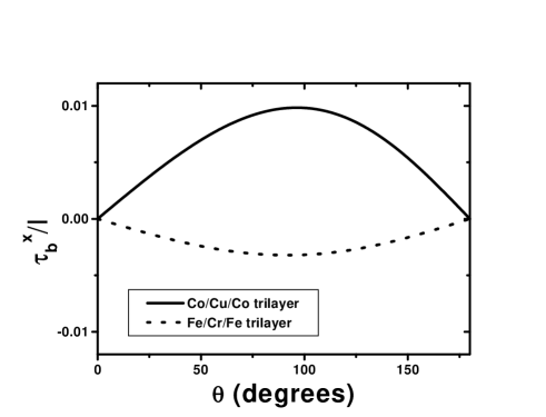
FIG. 8.: Torque per unit current as a function of $\theta$ for two different realistic systems. The solid line shows the Co-Cu-Co trilayer ($|t_{a\uparrow}|^{2}=0.73$, $|t_{a\downarrow}|^{2}=0.49$, $|t_{b\uparrow}|^{2}=0.68$, $|t_{b\downarrow}|^{2}=0.29$). The dashed line shows the Fe-Cr-Fe trilayer ($|t_{a\uparrow}|^{2}=0.48$, $|t_{a\downarrow}|^{2}=0.59$, $|t_{b\uparrow}|^{2}=0.30$, $|t_{b\downarrow}|^{2}=0.50$). In both cases $g_{\rm N}=N$ has been assumed. The thick layer is assumed to be semi-infinite while for the thin layer, only the interface properties have been taken into account. Numerical values are obtained from Ref. [11].

VI Conclusion

We have developed a theory for the spin-transfer-induced torques on the magnetic moments of a ferromagnet-normal-ferromagnet FNF trilayer system caused by a flowing current. Our theory deals with the effects of multiple scattering between the layers using the scattering matrices of the ferromagnet-normal metal interfaces as input parameters. We consider both the cases of a diffusive and ballistic normal metal spacer. Remarkably, in the diffusive case, the high-dimensional scattering matrices of the FN interfaces only appear through the reduced $4\times 4$ tensor products of Eq.(39) which greatly reduces the number of degrees of freedom of the theory (see also Ref. [13]). This reduction of the number of degrees of freedom allows us to make qualitative predictions about the role of the interface transparency, normal metal resistance etc., without detailed knowledge of the microscopic details of the system. However, for quantitative predictions, inclusion of the microscopic parameters in our theory, e.g. from ab initio calculations[11, 12] is still needed.

Having a complete theoretical description of the current-induced switching of magnetic domains in FN multilayers as a final goal, the theory here can be regarded as being an intermediate step. On the one hand, microscopic input is needed for the scattering matrices of the FN interfaces, as explained above. On the other hand, the output of our theory, the current-induced torques, needs to be combined with restoring (hysteretic) forces in a more phenomenological theory that describes the dynamics of the magnetic moments. Such a theory involves anisotropy forces and information about the mechanism by which the torque is exerted (spin wave excitation, local exchange field) – issues which are still subject of debate.[2, 3, 24, 26].

In this paper, we have focused on the effects of “spin filtering” as the mechanism for current-induced torque, i.e., the difference in the transmission and reflection probabilities for electrons with spins parallel and antiparallel to the moments of the ferromagnetic layers (the diagonal terms in the matrices for the reflection and transmission amplitudes, Eq.(19).) A different source of spin-dependent scattering, which we have not considered in detail, but which is included in our formalism, is that of spin-flip scattering – the off-diagonal terms in Eq.(19). Its effect can be twofold. In the normal spacer, it would decrease the effective polarization, and therefore the torque. However, in the ferromagnet, the rate of spin-flip scattering might be asymmetric with respect to minority and majority spins, and therefore spin-flip scattering may also be an additional source of torque. As the number of degrees of freedom involved is much larger than for spin filtering only, a realistic model for the scattering matrices in the ferromagnets would be a necessary starting point for a theory that would include the effect of spin-flip scattering. We leave such a theory for future work.

APPENDIX

A Derivation of Eq.(43)

In this appendix, we describe the calculation of Eq.(43) step by step.

First, we substitute the expression (30) for $\Omega$ into (34), and then formally expand the resulting equation in powers of the reflection matrices $r_{a}$, $r_{b}$, $r_{n}$ and $r^{\prime}_{n}$. Using the polar decomposition Eq.(37) for the reflection and transmission matrices $r_{n},t_{n},t^{\prime}_{n}$ and $r^{\prime}_{n}$ of the normal layer, we get a sum of many terms, each of which is of a form where contributions from N are alternated with those of F_a and F_b. Writing spin indices explicitly (summation over repeated indices is implied), we can write those terms as,

$${\rm Tr}_{N}\vec{\Sigma}_{ij}\left(A_{jk}\alpha B_{kl}\beta...\eta C_{sm}\right)\left(F^{\dagger}_{nm}\omega^{\dagger}...\delta^{\dagger}E_{pn}^{\dagger}\gamma^{\dagger}D_{ip}^{\dagger}\right),$$ (58)

where $A$, $B$, $C$, $D$, $E$, $F$ $\in\{r_{a},t_{a},r_{b},r^{\prime}_{b}...\}$ refer to the layer F_a and F_b while $\alpha$, $\beta$, $\gamma$, $\delta$, $\eta$, $\omega\in\{ui\sqrt{T}v,u\sqrt{1-T}u^{\prime},...\}$ refer to the normal layer.

We are now ready to do the average of Eq.(58) over the matrices $u,u^{\prime},v$ and $v^{\prime}$ using the diagrammatic technique of Ref. [22] (In leading order in $N$ these integrals reduce to the application of wick theorem.) Doing so, each of the $\alpha,\beta,...$ has to be put in correspondence with one of the $\gamma^{\dagger},\delta^{\dagger}$, etc. To leading order in $N$, only the ladder diagram survives, in which $\alpha=\gamma$, $\beta=\delta$, $\eta=\omega$,… and hence, $A=D$, $B=E$, $C=F$,… Thus, after averaging, we get terms like:

$${\rm Tr}_{N}\left[\vec{\Sigma}_{ij}\right]\frac{1}{N}{\rm Tr}_{N}\left[A_{jk}A_{ip}^{\dagger}\right]a\frac{1}{N}{\rm Tr}_{N}\left[B_{kl}B_{pn}^{\dagger}\right]b$$ (59)

$$...\ \ \ c\frac{1}{N}{\rm Tr}_{N}\left[C_{sm}C_{nm}^{\dagger}\right],$$ (60)

where $a,b,c,...$ stands for either $\frac{1}{N}{\rm Tr}T$ or $\frac{1}{N}{\rm Tr}(1-T)$.

To leading order in $N$, the average over $T$ can now be done by simply replacing $a,b,c,...$ by their average value $g_{\rm N}/N$ or $1-g_{\rm N}/N$ where $g_{\rm N}$ is the average conductance (per spin) of the normal layer, in unit of $e^{2}/h$.

Finally, denoting $\lambda=(i,j)$ and $\mu=(k,p)$, let us now introduce $4\times 4$ matrices $\hat{A}$, $\hat{B}$, $\hat{C}$,… that are defined as:

$$\hat{A}_{\lambda\mu}=\frac{1}{N}{\rm Tr}_{N}\left[A_{ik}A_{jp}^{\dagger}\right],$$ (61)

and $\hat{\vec{\Sigma}}$ is defined as

$$\hat{\vec{\Sigma}}_{\lambda\mu}=\delta_{kp}{\rm Tr}_{N}\vec{\Sigma}_{ji}.$$ (62)

In term of these new matrices, eq.(59) now reads as a simple matrix product:

$${\rm Tr}_{4}\hat{\vec{\Sigma}}\hat{A}\hat{\alpha}\hat{B}\hat{\beta}...\hat{\eta}\hat{C},$$ (63)

with $\hat{\alpha}$, $\hat{\beta}$, $\hat{\eta}$,…$\in\{g_{\rm N}/N,1-g_{\rm N}/N\}$. Equation (63) is formally equal to the expansion of $\Omega$ (see Eq.(58)) except that we are now dealing with “hat” matrices. Therefore, we can now resum all the terms of the expansion and get Eq. (43).

B Ballistic normal layer: a pedestrian approach

If N is very clean, and the interfaces are very flat, it is reasonable to assume that the electrons propagate ballistically inside the normal layer. The different modes will not be mixed in that case, and the electron wavefunction only picks up a phase factor $e^{ik_{i}L}$ where $L$ is the width of N and $k_{i}$ the momentum of channel $i$. For a sufficiently thick normal layer (i.e. $L\gg\lambda_{F}$), small fluctuations of $k_{i}$ lead to an arbitrary change in the phase factor, and it is justified to consider $e^{ik_{i}L}$ as a random phase and to average over it. This is different from the case of a disordered metal spacer, where the average involves unitary matrices $u$, $u^{\prime}$… that mix the channels, cf Eq.(37). In the case where $r_{a\downarrow}$, $r_{a\uparrow}$,… are proportional to the identity matrix (i.e. the reflection amplitudes do not depend on the channel), the ballistic model reduces to the disordered model of Eq. (43) for $g_{\rm N}=N$.

The reflection matrices of N being zero, the matrix $\Omega$ reads:

$$\Omega=e^{ik_{i}L}\frac{1}{1-e^{2ik_{i}L}r_{a}r^{\prime}_{b}}t^{\prime}_{a}.$$ (64)

Neglecting spin-flip scattering, denoting $z=e^{2ik_{i}L}$, and choosing $r_{a11}=r_{a\uparrow}$, $r_{a22}=r_{a\downarrow}$,… where $r_{a\uparrow}$, $r_{a\downarrow}$,… are diagonal matrices, one gets after some algebra:

$$\frac{\partial\tau_{b}^{x}}{\partial V_{0}}(z)=-\frac{e\nu}{4\pi}{\rm Tr\ Re\ }\frac{A(z)}{z|D(z)|^{2}}\sin\theta,$$ (65)

where $A(z)$ and $D(z)$ stand for:

$$A(z) = \left(1-t^{\prime}_{b\uparrow}t^{\prime*}_{b\downarrow}-r^{\prime}_{b\uparrow}r^{\prime*}_{b\downarrow}\right)$$ (66)

$$( |t^{\prime}_{a\uparrow}|^{2}(1-zr^{\prime}_{b\downarrow}r_{a\downarrow})(z-r^{\prime*}_{b\uparrow}r_{a\downarrow}^{*})$$ (67)

$$- \left.|t^{\prime}_{a\downarrow}|^{2}(1-zr_{b\downarrow}r_{a\uparrow})(z-r^{\prime*}_{b\uparrow}r_{a\uparrow}^{*})\right),$$ (68)

$$D(z) = 1-z\left[\cos^{2}\frac{\theta}{2}(r_{a\uparrow}r^{\prime}_{b\uparrow}+r_{a\downarrow}r^{\prime}_{b\downarrow})\right.$$ (69)

$$+ \left.\sin^{2}\frac{\theta}{2}(r_{a\downarrow}r^{\prime}_{b\uparrow}+r_{a\uparrow}r^{\prime}_{b\downarrow})\right]$$ (70)

$$+ z^{2}r_{a\downarrow}r_{a\uparrow}r^{\prime}_{b\downarrow}r^{\prime}_{b\uparrow}.$$ (71)

A similar formula can be written for the conductance $g(z)$:

$$g=\frac{e^{2}}{h}{\rm Tr\ }\frac{B(z)}{z|D(z)|^{2}},$$ (72)

with:

$$B(z) = |t^{\prime}_{a\uparrow}|^{2}|t^{\prime}_{b\uparrow}|^{2}\cos^{2}\frac{\theta}{2}(1-zr_{a\downarrow}r^{\prime}_{b\downarrow})(z-r_{a\downarrow}^{*}r^{\prime*}_{b\downarrow})$$ (73)

$$+ |t^{\prime}_{a\uparrow}|^{2}|t^{\prime}_{b\downarrow}|^{2}\sin^{2}\frac{\theta}{2}(1-zr_{a\downarrow}r^{\prime}_{b\uparrow})(z-r_{a\downarrow}^{*}r^{\prime*}_{b\uparrow})$$ (74)

$$+ |t^{\prime}_{a\downarrow}|^{2}|t^{\prime}_{b\uparrow}|^{2}\sin^{2}\frac{\theta}{2}(1-zr_{a\uparrow}r^{\prime}_{b\downarrow})(z-r_{a\uparrow}^{*}r^{\prime*}_{b\downarrow})$$ (75)

$$+ |t^{\prime}_{a\downarrow}|^{2}|t^{\prime}_{b\downarrow}|^{2}\cos^{2}\frac{\theta}{2}(1-zr_{a\uparrow}r^{\prime}_{b\uparrow})(z-r_{a\uparrow}^{*}r^{\prime*}_{b\uparrow}).$$ (76)

Taking the average over the phases now amounts to coutour integration for $z$:

$$\langle f\rangle=\frac{1}{2\pi i}\oint\frac{dz}{z}\ \ f(z),$$ (77)

where the integration is done along the unit circle. The result is then given by the sum of the poles that are inside the unit circle. The two poles of $D(z)$ are outside the unit circle, while the two poles $z_{1}$ and $z_{2}$ of $z^{2}D\left(\frac{1}{z}\right)$ are inside the circle. They are given by:

$$z_{i} = \frac{1}{2}\cos^{2}\frac{\theta}{2}(r_{a\uparrow}r^{\prime}_{b\uparrow}+r_{a\downarrow}r^{\prime}_{b\downarrow})+\sin^{2}\frac{\theta}{2}(r_{a\downarrow}r^{\prime}_{b\uparrow}+r_{a\uparrow}r^{\prime}_{b\downarrow})$$ (78)

$$+ \frac{1}{2}(-1)^{i}\left[\cos^{4}\frac{\theta}{2}(r_{a\uparrow}r^{\prime}_{b\uparrow}-r_{a\downarrow}r^{\prime}_{b\downarrow})^{2}\right.$$ (79)

$$+ 2\cos^{2}\frac{\theta}{2}\sin^{2}\frac{\theta}{2}(r^{\prime}_{b\downarrow}r^{\prime}_{b\uparrow}(r_{a\uparrow}-r_{a\downarrow})^{2}+r_{a\downarrow}r_{a\uparrow}(r^{\prime 2}_{b\uparrow}+r_{a\downarrow}^{2}))$$ (80)

$$+ \left.\sin^{4}\frac{\theta}{2}(r_{a\downarrow}r^{\prime}_{b\uparrow}-r_{a\uparrow}r^{\prime}_{b\downarrow})^{2}\right]^{\frac{1}{2}}.$$ (81)

The averaged torque and conductance are then simply given by

$$\langle\frac{\partial\tau_{b}^{x}}{\partial V_{0}}\rangle=-\frac{e\nu}{4\pi}\frac{\sin\theta}{z_{1}-z_{2}}{\rm Tr\ }\left(\frac{A(z_{1})}{D(z_{1})}-\frac{A(z_{2})}{D(z_{2})}\right)$$ (82)

and

$$g=\frac{e^{2}}{h}\frac{1}{z_{1}-z_{2}}{\rm Tr\ }\left(\frac{B(z_{1})}{D(z_{1})}-\frac{B(z_{2})}{D(z_{2})}\right).$$ (83)

In the case where all the channels are not identical, these results can be generalized by introducing a $k$ dependence of the different transmission/reflection amplitudes.

REFERENCES

- [1] For a review, see the collection of articles in IBM J. Res. Dev. 42 (1998).
- [2] L. Berger, Phys. Rev. B 54, 9353 (1996).
- [3] J. Slonczewski, J. Magn. Magn. Mater. 159, L1 (1996).
- [4] We use the term “spin transfer” to describe the transfer, during the process of electron scattering, of spin angular momentum between an electron current and a magnet. The term should be used with care in describing the current-induced interaction between adjacent magnetic layers, because there is not a simple transfer of angular momentum from one layer to the other – spin may also flow away to infinity. The total magnetic moment of the two magnetic layers is therefore not conserved; see our discussion in section II.
- [5] M. Tsoi, A. G. M. Jansen, J. Bass, W.-C. Chiang, M. Seck, V Tsoi, and P. Wyder, Phys. Rev. Lett. 80, 4281 (1998); 81, 493 (1998) (E).
- [6] R. N. Louie, Ph.D. Thesis, Cornell University (1997). J. Z. Sun, J. Magn Magn Mater. 202, 157 (1999).
- [7] E. B. Myers, D. C. Ralph, J. A Katine, R. N. Louie, and R. A. Buhrman , Science 285, 867 (1999).
- [8] J. A. Katine, F. J. Albert, R. A. Buhrman, E. B. Myers, and D. C. Ralph, cond-mat/9908231, to appear in Phys. Rev. Lett.
- [9] J. C. Slonczewski, Proceedings of conference Frontiers in Magnetism 99 (FIM99), held in Stockholm, August 12-15th, 1999.
- [10] M. Tsoi, A. G. M. Jansen, J. Bass, W.-C. Chiang, V. Tsoi, and P. Wyder, preprint.
- [11] M. D. Stiles, J. Appl. Phys. 79, 5805 (1996); Phys. Rev. B. 54, 14679 (1996).
- [12] K. M. Schep, P.J. Kelly and G. E. W. Bauer, Phys. Rev. Lett. 74, 586 (1995). K. M. Schep, J. B. A. N. van Hoof, P. J. Kelly G. E. W. Bauer and J. E. Inglesfield, Phys. Rev. B 56 10805 (1997).
- [13] A. Brataas, Y. V. Nazarov and G. E. W. Bauer, Phys. Rev. Lett. 84 2481 (2000). D. Huertas Hernando, Y.V. Nazarov, A. Brataas and G. E. W. Bauer, cond-mat/0003382.
- [14] L. Berger, J. Appl. Phys 55, 1954 (1984).
- [15] C.W.J. Beenakker, Rev. Mod. Phys. 69, 731 (1997).
- [16] M. Büttiker and T. Christen in Quantum Transport in Submicron Structures, edited by B. Kramer, Kluwer (1996).
- [17] K. B. Hathaway and J. R. Cullen, J. Magn. Magn. Mater. 104-107, 1840 (1992).
- [18] J. C. Slonczewski, J. Magn. Magn. Mater. 126, 374 (1993).
- [19] P. Bruno, Phys. Rev. B. 52, 411 (1995).
- [20] D. M. Edwards, A. M. Robinson, and J. Mathon, J. Magn. Magn. Mater. 140-144, 517 (1995).
- [21] A. D. Stone, P. A. Mello, K. A. Muttalib, and J.-L. Pichard in Mesoscopic Phenomena in Solids, edited by B. L. Altshuler, P. A. Lee, and R. A. Webb (North Holland, Amsterdam, 1991).
- [22] P.W. Brouwer and C.W.J. Beenakker, J. Math. Phys. 37, 4904 (1996).
- [23] J. Slonczewski, J. Magn. Magn. Mater. 195, L261 (1999).
- [24] C. Heide, P.E. Zilberman and R.J. Elliot cond-mat/0005064.
- [25] In the notation of Ref. [3], the fraction of the channels that act as perfect filters is .
- [26] Ya. B. Bazaliy, B. A. Jones, and S.-C. Zhang, Phys. Rev. B 57, R3213 (1998).