Charge occupancy of two interacting electrons on artificial molecules – exact results

Abstract

We present exact solutions for two interacting electrons on an artificial atom and on an artificial molecule made by one and two (single level) quantum dots connected by ideal leads. Specifically, we calculate the accumulated charge on the dots as function of the gate voltage $\epsilon_{0}$, for various strengths of the electron-electron interaction $U$ and of the hybridization between the dots and the (one-dimensional) leads $\gamma$. For $\gamma<1$ and $2(\gamma-1)\equiv\epsilon_{00}<\epsilon_{0}<0$, there are no bound states. As $\epsilon_{0}$ decreases beyond $\epsilon_{00}$, the accumulated charge $P$ in the two-electron ground state increases in gradual steps from 0 to 1 and then to 2. The values $P\sim 0$ represent an “insulating” state, where both electrons are bound to shallow states on the impurities. The value of $P\approx 1$ corresponds to a “metal”, with one electron localized on the dots and the other extended on the leads. The value of 2 corresponds to another “insulator”, with both electrons strongly localized. The width of the “metallic” regime diverges with $U$ for the single dot, but remains very narrow for the double dot. These results are contrasted with the simple Coulomb blockade picture.

]

I Introduction

Much of the early work on quantum dots concentrated on large dots, which may contain many electrons, in the limit of very weak coupling between the dots and the leads, where one can employ the simple Coulomb blockade picture. [2] In that limit, the energy cost of adding a single electron to the dot is of order of the excess energy for the added charge. For a total of two electrons, this is of the order of the Coulomb repulsion between the two electrons. One expects that for a good contact between the dots and the leads this energy cost will be reduced. However, the study of a general coupling strength presents a great challenge. The case of an ‘open’ dot, connected by quantum point contacts to a two-dimensional electron gas, [3] has been analyzed using bozonization techniques and mapping of the Hamiltonian onto the two- and four-channel Kondo problem. [4]

It has only recently become possible to also study small quantum dots, which have a small number of states and contain a small number of electrons. [5, 6] Such a small dot, connected to external leads, is similar to a donor in a doped semiconductor: both may be modeled as an ‘impurity’ connected to external leads. [7] A set of such quantum dots, or an artificial molecule, can then be modeled by a set of such ‘impurities’. In what follows, we sometimes interchange the terms ‘dot’ and ‘impurity’. It is usually assumed that the electrons interact with each other only when they are on the same quantum dot, and behave as free electrons when they are on the leads. In what follows we therefore assume a contact interaction, which exists only on the dots, and present exact results for the case of two electrons. Given the difficulties in solving the general problem, such analytical results (even for the most simple configruations) are helpful. They are particularly useful for nanostructures, where one might design controlled experiments. [5, 6]

We have recently reported on several exact results for two interacting electrons on a general number of dots ${\cal N}$, which are modeled as ‘impurities’ which have single electronic states: we presented a general scheme for finding the eigenenergies, and presented some results for the spectra of a single dot. [8] We have also discussed the exact two-electron current through a single dot. [9] Here we generalize these results, with emphasis on the charge accumulated on each quantum dot and on its relationship with the Coulomb blockade picture. We then devote most of this paper to discuss the more complex case of a double dot. Such a double dot, with one state per dot, has recently been proposed as a possible candidate for the two-qubit entanglement required for quantum computation. [10] The case of two coupled quantum dots is also amenable to experiments. [11]

In our earlier work [8], we showed that the spectrum and the wave functions of the two interacting electrons can be obtained in terms of the energy spectrum and the wave functions of the single-electron Hamiltonian. We reproduce these results in section II in a slightly different method, and use them to obtain new results for the charge occupancies on the quantum dots. The next two sections are devoted to the study of specific configurations: a single dot, and a system made up of two dots, separated by a distance $R$. The single-electron spectra of these two configurations, required for the study of the two electron one, are discussed in the Appendix.

II Two interacting electrons – general scheme

As has been demonstrated in Ref. [8], the knowledge of the spectrum of the single-electron Hamiltonian is sufficient for deducing the spectrum and the wave functions of two interacting electrons, for any number ${\cal N}$ of dots. Basically, we start with the Hamiltonian

$${\cal H}={\cal H}_{\rm se}+{\cal H}_{\rm int}.$$ (1)

The spin-independent single-electron part ${\cal H}_{\rm se}$ involves site energies $\epsilon_{\rm i}$ on the dots (${\rm i}=1,~{}2,...,{\cal N}$) and zero on the lead sites, and also nearest neighbor hopping matrix elements $t_{n,m}$ which assume special values near the dots. This part is diagonalized by the eignenergies $\{\epsilon_{a}\}$ and the corresponding eigenfunctions $\{\phi_{a}(n)\}$.

For simplicity, we assume that the two electrons interact only when they are both on the same dot i, with interaction energy $U({\rm i})$ (though the method of solution can be extended for other types of interactions):

$${\cal H}_{\rm int}=\sum_{\rm i}U({\rm i})c^{\dagger}_{{\rm i}\uparrow}c_{{\rm i}\uparrow}c^{\dagger}_{{\rm i}\downarrow}c_{{\rm i}\downarrow}.$$ (2)

Using the single-electron eigenstates, the two-electron Hamiltonian takes the form

$${\cal H}=\sum_{a\sigma}\epsilon_{a}c^{\dagger}_{a\sigma}c_{a\sigma}+\sum_{{\rm i}}\sum_{abcd}U_{acbd}({\rm i})c^{\dagger}_{a\uparrow}c_{b\uparrow}c^{\dagger}_{c\downarrow}c_{d\downarrow},$$ (3)

$$U_{acbd}({\rm i})=U({\rm i})\phi^{\ast}_{a}({\rm i})\phi^{\ast}_{c}({\rm i})\phi_{b}({\rm i})\phi_{d}({\rm i}).$$ (4)

Here, $c^{\dagger}_{a\sigma}\equiv\sum_{n}\phi_{a}(n)c^{\dagger}_{n\sigma}$ creates an electron in the state $a$ with spin $\sigma$.

For such a contact electron-electron interaction, one is interested only in the singlet state of the two electrons (the energies of the two electrons in the triplet state are simply given by the non-interacting sums $\epsilon_{a}+\epsilon_{b}$). We hence write for the two-electron singlet wave function

$$|\Psi\rangle=\sum_{ab}X_{ab}(E)c^{\dagger}_{a\uparrow}c^{\dagger}_{b\downarrow}|0\rangle,$$ (5)

where $|0\rangle$ is the vacuum and $X_{ab}=X_{ba}$. The Schrödinger equation

$${\cal H}|\Psi\rangle=E|\Psi\rangle$$ (6)

then yields

$$\sum_{ab}\Bigl{(}E-\epsilon_{a}-\epsilon_{b}\Bigr{)}X_{ab}(E)c^{\dagger}_{a\uparrow}c^{\dagger}_{b\downarrow}|0\rangle$$ (7)

$$= \sum_{{\rm i}}\sum_{aba^{\prime}b^{\prime}}X_{ab}(E)U_{a^{\prime}b^{\prime}ab}({\rm i})c^{\dagger}_{a^{\prime}\uparrow}c^{\dagger}_{b^{\prime}\downarrow}|0\rangle.$$ (8)

Multiplying this equation from the left by $\langle 0|c_{b^{\prime\prime}\downarrow}c_{a^{\prime\prime}\uparrow}$ gives

$$X_{ab}(E)=\sum_{{\rm i}}\sum_{a^{\prime}b^{\prime}}\frac{U_{aba^{\prime}b^{\prime}}({\rm i})X_{a^{\prime}b^{\prime}}(E)}{E-\epsilon_{a}-\epsilon_{b}}.$$ (9)

The simple form of the matrix elements of the contact interaction [see Eq. (4)] allows us to rewrite Eq. (9) as a set of ${\cal N}$ linear equations: Defining the quantities

$$A_{{\rm i}}(E)=\sum_{ab}\phi_{a}({\rm i})\phi_{b}({\rm i})X_{ab}(E)$$ (10)

(which represent the amplitudes of $|\Psi\rangle$ for the singlet state with both electrons on site i, denoted by $|{\rm i,i}\rangle$), one arrives at

$$A_{{\rm i}}(E)=\sum_{{\rm i}^{\prime}}U({\rm i}^{\prime})G_{E}({\rm i,i;i^{\prime},i^{\prime}})A_{{\rm i}^{\prime}}(E),$$ (11)

in which $G_{E}({\rm i,i;i^{\prime},i^{\prime}})$ is the two-particle Green’s function of two non-interacting electrons,

$$G_{E}({n_{1},n_{2};n_{1}^{\prime},n_{2}^{\prime}})=\sum_{ab}\frac{\phi_{a}(n_{1})\phi_{b}(n_{2})\phi^{\ast}_{a}(n_{1}^{\prime})\phi^{\ast}_{b}(n_{2}^{\prime})}{E-\epsilon_{a}-\epsilon_{b}},$$ (12)

calculated at the impurity locations. [12] The determinant of Eqs. (11) gives the eigenenergies $\{E\}$ of the two interacting electrons, and in particular determines the ground state energy, $E_{G}$. The coefficients $X(E)$ are then obtained from Eq. (9), which can be rewritten as

$$X_{ab}(E)=\sum_{{\rm i}}\frac{U({\rm i})\phi^{\ast}_{a}({\rm i})\phi^{\ast}_{b}({\rm i})A_{\rm i}(E)}{E-\epsilon_{a}-\epsilon_{b}}.$$ (13)

Substituting this result into Eq. (5), it is easy to check that

$$|\Psi\rangle=\sum_{\rm i}U({\rm i})A_{\rm i}(E)\sum_{n_{1},n_{2}}G_{E}(n_{1},n_{2};{\rm i},{\rm i})|n_{1},n_{2}\rangle,$$ (14)

$|n_{1},n_{2}\rangle$ is a singlet state with one electron at site $n_{1}$ and the other at site $n_{2}$. Note that Eq. (11) determines the $A_{\rm i}$’s only up to a multiplicative constant. This constant should be determined by the normalization of $|\Psi\rangle$, i. e. from the condition $\sum_{ab}|X_{ab}(E)|^{2}=1$. Such solutions will be discussed in some detail below.

The electronic states on a quantum dot are commonly probed by varying the gate voltages on the dots, represented here by the $\epsilon_{\rm i}$’s, and measuring the conductance. Alternatively, one may probe the total charge on the dots, by measuring the capacitance when the gate voltage is changed.[5] The total charge on the dots, in the state $|\Psi\rangle$, is given by (in units of the electron charge, $e$)

$$P = \sum_{\sigma}\sum_{{\rm i}=1}^{{\cal N}}\langle\Psi|c^{\dagger}_{{\rm i}\sigma}c_{{\rm i}\sigma}|\Psi\rangle$$ (16)

$$\equiv\langle\Psi|\sum_{{\rm i}=1}^{{\cal N}}\sum_{ab}\phi^{\ast}_{a}({\rm i})\phi_{b}({\rm i})\sum_{\sigma}c^{\dagger}_{a\sigma}c_{b\sigma}|\Psi\rangle.$$

Using Eq. (5), we obtain

$$P=2\sum_{{\rm i}}\sum_{abc}\phi^{\ast}_{a}({\rm i})\phi_{b}({\rm i})X^{\ast}_{ac}(E)X_{bc}(E).$$ (17)

Alternatively, we note that

$$P=\sum_{\rm i}\frac{\partial E}{\partial\epsilon_{\rm i}}.$$ (18)

This follows from first-order perturbation theory: writing $E=\langle\Psi|{\cal H}|\Psi\rangle$, the derivative with respect to $\epsilon_{\rm i}$ becomes $\langle\Psi|c^{\dagger}_{{\rm i}\sigma}c_{{\rm i}\sigma}|\Psi\rangle$. In the following sections, we will use these results to discuss the ground state of simple quantum dot systems occupied by two electrons.

An important technical advantage of the representation of the two-electron spectrum in terms of the two-particle Green’s function of the non-interacting system, is that the latter can be expressed in terms of the single-particle Green’s function. The spectral representation of the single-particle Green’s function, $g_{\omega}(n;n^{\prime})$, is

$$g_{\omega}(n;n^{\prime})=\sum_{a}\frac{\phi_{a}(n)\phi^{\ast}_{a}(n^{\prime})}{\omega+i\zeta-\epsilon_{a}},$$ (19)

where $\zeta\rightarrow 0^{+}$. In conjunction with Eq. (12), one finds [9]

$$G_{E}(n_{1},n_{2};n_{1}^{\prime},n_{2}^{\prime})$$ (20)

$$= -\frac{1}{\pi}\int_{-\infty}^{\infty}d\omega g_{E-\omega}(n_{1};n_{1}^{\prime})\Im g_{\omega}(n_{2};n_{2}^{\prime})$$ (21)

$$= \frac{i}{2\pi}\int_{-\infty}^{\infty}d\omega g_{E-\omega}(n_{1};n_{1}^{\prime})g_{\omega}(n_{2};n_{2}^{\prime}),$$ (22)

where the last equality follows from the Kramers-Kronig relations. The relation (22) is very useful in the detailed calculations of the ground state properties, because the single-particle Green’s functions are relatively easy to find. We give in Appendix A the details of the single-particle Green’s functions required for the dot configurations investigated in this paper.

III a single dot on a one-dimensional wire

We model a single dot on a one-dimensional wire by a single impurity, located at site 0, which has the on-site energy $\epsilon_{0}$, and is coupled to two ideal one-dimensional leads, with the amplitude $t_{0}$ for tunneling between the impurity and its nearest neighbors on the leads. [7] Both these parameters are experimentally accesssible: $\epsilon_{0}$ models the plunger gate voltage on the dot, while $t_{0}$ is related to the transmittance (or conductance) of the barriers between each dot and the leads, which can be varied by changing the gate voltages on these barriers. The corresponding amplitudes between sites inside the leads are equal to $-t$. Although some aspects of the solution of this problem were discussed in Ref. [8], we present here an alternative derivation, which is more adapted to the calculation of the occupation $P$ and to the more complicated case of two dots.

As shown in Appendix A,[8] the single-particle Hamiltonian of such a system has none, one or two bound states, depending on the values of the “gate voltage” $\epsilon_{0}$ and the “hybridization” $t_{0}^{2}\equiv\gamma$ (energies are measured in units of $t$). For the sake of concreteness, we concentrate on the region where there is only one bound state below the band, of energy $\epsilon_{\beta}<-2$. This occurs for $\epsilon_{0}<\epsilon_{00}\equiv 2(\gamma-1)$ (see Appendix A).

In the simple case of a single ‘impurity’, Eq. (11) reduces to a single equation, and the eigenenergies $\{E\}$ of the two interacting electrons are given by the solutions of

$$\frac{1}{U}=G_{E}(0,0;0,0)=\sum_{ab}\frac{|\phi_{a}(0)|^{2}|\phi_{b}(0)|^{2}}{E-\epsilon_{a}-\epsilon_{b}}.$$ (23)

It is easy to deduce the beahvior of $G_{E}$ as function of the two-electron energy $E$ from this equation. $G_{E}$ is negative for $E<2\epsilon_{\beta}$, decreasing from 0 to $-\infty$ as $E$ increases from $-\infty$ towards $2\epsilon_{\beta}$. As $E$ crosses this value, it jumps to $+\infty$ and then decreases. The value $E=-2+\epsilon_{\beta}$ marks the beginning of the two-particle continuous band states: one electron is bound and the other is in the continuum.

As discussed in Ref. [8], $G_{E}$ is finite at $E=-2+\epsilon_{\beta}$ in the thermodynamic limit of infinite leads, due to the vanishing of the band state wavefunction $\phi_{k}$ (with energy $\epsilon_{k}=-2\cos k$) at the impurity site ${\rm i}=0$ for $k=0$. This value of $G$ determines whether there is or there is not a bound state of the two interacting electrons: When $1/U<G_{-2+\epsilon_{\beta}}$, then Eq. (23) has no solution for $E<-2+\epsilon_{\beta}$, and there is no doubly occupied bound state below the band. One of the electrons is then in a band state. The behavior of $G$ at $E=-2+\epsilon_{\beta}$, as function of $\epsilon_{0}$, is plotted in Fig. 1. Since $G_{E=-2+\epsilon_{\beta}}$ has a maximum, $G_{\rm max}$, there is always a doubly occupied bound state (or an “insulator”) for $U<1/G_{\rm max}$. For larger $U$, the equation $G_{-2+\epsilon_{\beta}}=1/U$ has two solutions, $\epsilon_{0,-}$ and $\epsilon_{0,+}$ (which depend on $U$). For $\epsilon_{0,-}<\epsilon_{0}<\epsilon_{0,+}$ one has no doubly occupied bound state, and the ground state of the two electrons lies in the continuum (i. e. represents a “metal”). Then, as the on-site energy $\epsilon_{0}$ becomes more attractive, the bound state of the two electrons re-appears. As seen from Fig. 1, $\epsilon_{0,-}$ diverges to $-\infty$ when $U\rightarrow\infty$, and this re-entrance then disappears. The region between $\epsilon_{0,-}$ and $\epsilon_{0,+}$ becomes narrower as $\gamma$ increases, and for finite $U$ it always disappears above some critical hybridization $\gamma_{c}$ (which diverges to $\infty$ as $U\rightarrow\infty$). [8]

These “insulator to metal” [13] transitions of the two-electron ground state, from being bound to being in the continuum and back, are reflected in the occupancy $P$ of the dot in the ground state [see Eq. (18)]. To find $P$, we re-write the equation for the ground energy $E_{G}$ in the form

$$\frac{1}{U}=-\frac{1}{\pi}\int_{-\infty}^{\infty}d\omega(D_{E_{G}-\omega})^{-1}\Im(D_{\omega})^{-1},$$ (24)

where we have used Eq. (22), and the results for $g_{\omega}$ relevant for this geometry [Eq. (A10)]. The imaginary part appearing in this expression has a delta-function contribution coming from the single-electron bound energy, and the contribution arising from the band states. Separating these two, we have

$$\frac{1}{U} = \frac{r(\epsilon_{\beta})}{D_{E_{G}-\epsilon_{\beta}}}$$ (25)

$$- \frac{1}{\pi}\int_{-2}^{2}d\omega(D_{E_{G}-\omega})^{-1}\Im(D_{\omega})^{-1},$$ (26)

where $r(\omega)=(\partial D_{\omega}/\partial\omega)^{-1}$ is the residue at the bound energy pole $\omega=\epsilon_{\beta}$. It is now straightforward to differentiate all terms in (26) with respect to $\epsilon_{0}$, and obtain $P=\partial E_{G}/\partial\epsilon_{0}$.

We have solved Eq. (26) for $E_{G}$, by calculating the integral numerically. We have then computed the variation of the occupancy $P$ as function of the gate voltage $\epsilon_{0}$, and the results are shown in Fig. 2, for a comparatively large hybridization, and in Fig. 3, for a small hybridization $\gamma$. Generally, $P$ starts at 0 at $\epsilon_{0}=\epsilon_{00}=2(\gamma-1)$, when the single electron bound state just moves below the band (with the inverse localization length $\kappa_{\beta}=0$, i. e. zero weight on the impurity). $P$ then grows as $\epsilon_{0}$ decreases. As seen from Fig. 1, $\epsilon_{0,+}$ is quite close to $\epsilon_{00}=2(\gamma-1)$, due to the steepness of $G$ [$G$ diverges to $-\infty$ as $\epsilon_{0}\uparrow 2(\gamma-1)$]. Therefore, the first transition into the “metallic” phase, at $\epsilon_{0,+}$, occurs when the localization lengths of the two bound electrons are still quite large, and their weights on the impurity (and thus also $P$) are relatively small. The calculation of $P$ in this regime is not easy, due to numerical problems related to the above mentioned steepness. In any case, $P$ reaches values close to 1 somewhere inside the “metallic” phase, i. e. for $\epsilon_{0,-}<\epsilon_{0}<\epsilon_{0,+}$. We note that in the first “insulating” phase, which appears at $\epsilon_{0,+}<\epsilon_{0}<2(\gamma-1)$, both electrons are bound on very shallow states, hence the small value of $P$. Thus, it is not enough to know $P$ in order to determine the transport nature of the system. As $\epsilon_{0}$ crosses below $\epsilon_{0,-}$, into the second “insulating” phase, $P$ gradually increases towards 2, reflecting the strongly bound state of the two electrons. This gradual increase becomes steeper as the hybridization $\gamma$ becomes smaller, and the width of the “metallic” single electron occupancy regime (of order $\epsilon_{0,+}-\epsilon_{0,-}$) increases with increasing $U$. Both of these facts are in qualitative accordance with the Coulomb blockade picture (where usually the derivative of $P$ with respect to the gate voltage has peaks whose width increases with the hybridization and whose inter-peak distance increases with $U$). [2, 4] In fact, the distance between the $N$’th and the $(N-1)$’th peaks is usually interpreted as the energy cost of adding the $N$’th electron. However, it is usually very difficult to obtain quantitative estimates for these quantities in that picture. Furthermore, the similarity of our results to the simple Coulomb blockade picture is completely lost as $\gamma$ increases towards and beyond $\gamma_{c}$: the width of the “metallic” regime then shrinks, and the there is a continuous gradual increase of $P$ from 0 to 2.

Returning to Eq. (14), we now observe that for a single impurity, the two-electron state is given by

$$|\Psi\rangle=UA\sum_{n_{1},n_{2}}G_{E}(n_{1},n_{2};0,0)|n_{1},n_{2}\rangle,$$ (27)

where $A$ is found from the normalization. One can now use Eq. (22) and the single electron Green’s functions $g_{\omega}(n;0)$ to obtain $|\Psi\rangle$. For the bound ground state, the results show an exponential decay of the amplitudes as either electron moves away from the impurity.

IV Two dots on a one-dimensional wire

Two dots are modeled by two ‘impurities’, connected to each other and to the outside by ideal linear leads. The presence of two impurities gives rise to up to four single-particle bound states. For simplicity, we consider two identical impurities, each having the same on-site energy $\epsilon_{0}$, which are located at sites $\ell$ and $r$, and are separated by a distance $R$ ($R\geq 2$). Confining ourselves again to the configuration where the bound states appear only below the band, the first bound state appears when $\epsilon_{0}$ is smaller than $\epsilon_{00}=2(\gamma-1)$, while the second appears only for $R>R_{c}$, where

$$R_{c}=2\gamma/(2\gamma-2-\epsilon_{0}).$$ (28)

At fixed $R$, there exists a single bound state below the band only in the narrow regime

$$2(\gamma-1-\gamma/R)<\epsilon_{0}<2(\gamma-1).$$ (29)

We also restrict ourselves to the regime with $\epsilon_{0}<2(1-\gamma)$, so that there are no bound states above the band (see Appendix A).

Assuming the on-site Coulomb interaction to be identical on the two impurities, $U(\ell)=U(r)\equiv U$, Eqs. (11) yield

$$A_{\ell}(E) = UG_{E}({\rm d})A_{\ell}(E)+UG_{E}({\rm nd})A_{r}(E),$$ (30)

$$A_{r}(E) = UG_{E}({\rm nd})A_{\ell}(E)+UG_{E}({\rm d})A_{r}(E),$$ (31)

where the labels d and nd stand for the diagonal and the nondiagonal elements of the matrix. By symmetry,

$$G_{E}({\rm d}) \equiv G_{E}(\ell,\ell;\ell,\ell)=G_{E}(r,r;r,r),$$ (32)

$$G_{E}({\rm nd}) \equiv G_{E}(\ell,\ell;r,r)=G_{E}(r,r;\ell,\ell).$$ (33)

The eigenenergies of the two interacting electrons are given by the solutions of the two equations

$$\frac{1}{U}=G_{E}({\rm d})\pm G_{E}({\rm nd})\equiv G^{\pm}_{E},$$ (34)

and the corresponding solutions obey

$$A^{\pm}_{\ell}(E)=\pm A^{\pm}_{r}(E).$$ (35)

It is instructive to rewrite these equations in terms of the single-electron wave functions, using Eq. (12). In the symmetric molecule case, one can divide the solutions into even and odd single-electron wave functions, with $\phi_{a}(\ell)=\pm\phi_{a}(r)$. From Eq. (12) it now follows that

$$G_{E}^{\pm}=\sum_{ab}\frac{[\phi_{a}(\ell)\phi_{b}(\ell)\pm\phi_{a}(r)\phi_{b}(r)]\phi^{\ast}_{a}(\ell)\phi^{\ast}_{b}(\ell)}{E-\epsilon_{a}-\epsilon_{b}}.$$ (36)

Thus, it is clear that $G_{E}^{+}$ contains only pairs of states where both $a$ and $b$ are even or odd, while $G_{E}^{-}$ contains only mixed combinations, where one state is even and the other is odd. It thus follows that the solutions of the two-electron problem divide into two separate families: the solutions of $G_{E}^{+}=1/U$ involve only even-even and odd-odd single electron states, while those of $G_{E}^{-}=1/U$ involve only even-odd states: the coefficients in Eq. (5) will split into two separate families, associated with the different solutions of Eqs. (34). This can be easily seen by substituting Eq. (35) into Eq. (14).

To discuss the two-electron energies, we need to analyze the $E$-dependence of $G_{E}^{\pm}$. This depends on $R$: For $R>R_{c}$, there exist two single-electron bound states, the even $\phi_{\beta+}$ and the odd $\phi_{\beta-}$. Thus, $G_{E}^{+}$ decreases from $\infty$ to $-\infty$ as $E$ increases from $2\epsilon_{\beta+}$ towards $2\epsilon_{\beta-}$. Therefore, in this case the equation $G_{E}^{+}=1/U$ always has a discrete solution, with $E$ between $2\epsilon_{\beta+}$ and $2\epsilon_{\beta-}$. In the same case, $G_{E}^{-}$ decreases from $\infty$ towards a finite value as $E$ increases from $\epsilon_{\beta+}+\epsilon_{\beta-}$ towards the bottom of the continuum $-2+\epsilon_{\beta+}$ (which contains both even and odd states). The new lowest even-odd state may thus be either “insulating” or “metallic”, depending on the sign of $1/U-G^{-}_{-2+\epsilon_{\beta+}}$. However, the energy of this even-odd state is always above the lowest triplet energy, which is equal to the non-interacting value $\epsilon_{\beta+}+\epsilon_{\beta-}$. From our numerical calculations we observe that $G_{E}^{+}$ is negative at this lowest triplet energy. Therefore, the lowest solution of $G_{E}^{+}=1/U$ is the ground state of the two-electron problem, which is thus a singlet. In a way, this might have been expected: breaking the system into two parts, by removing a bond in the middle between the two dots, one ends up with separate “atomic” states on each side, each coupled to its own lead. Each side can then contain one electron with either spin up or spin down. However, switching on the hopping $t_{h}$ between the two sides would lower the energy of the singlet state, similarly to the antiferromagnetic ground state of the Hubbard model; to lowest order in $t_{h}$, the “exchange” difference between the triplet and singlet states is of order $t_{h}^{2}/U$.[14] It is interesting to note that in our case there exists a finite difference between the singlet and the triplet even in the limit $U\rightarrow\infty$, since we find that $G^{+}_{\epsilon_{\beta+}+\epsilon_{\beta-}}$ is strictly negative. It would be interesting to study generalizations of our simple model, e. g. including interdot Coulomb and exchange interactions, which would allow an interchange of the singlet and triplet ground states. [15]

The only chance to find a “metallic” ground state is thus for $R<R_{c}$, when there exists only one single-electron bound state below the band. This limits the possible range of parameters to that in Eq. (29). In this regime, $G_{E}^{-}$ yields no doubly bound state, and $G_{E}^{+}$ yields one only if $G^{+}_{-2+\epsilon_{\beta+}}<1/U$. Note that this regime becomes narrower (in terms of $\epsilon_{0}$) as $R$ increases. It is therefore interesting to find the borderline in the parameter space, at which $G^{+}_{-2+\epsilon_{\beta+}}=1/U$. Inside this broderline, the ground energy of the two electrons is in the continuum, i. e. “metallic”.

To calculate $G_{E}^{\pm}$, we use Eq. (22) and the results (A21) and (A24) of Appendix A:

$$G^{+}_{E}=G_{E}({\rm d})+G_{E}({\rm nd})$$ (37)

$$= -\frac{1}{2\pi}\int d\omega\Biggl{(}\frac{1}{D_{E-\omega}^{-}}\Im\frac{1}{D^{-}_{\omega}}+\frac{1}{D_{E-\omega}^{+}}\Im\frac{1}{D^{+}_{\omega}}\Biggr{)},$$ (39)

$$G^{-}_{E}=G_{E}({\rm d})-G_{E}({\rm nd})$$

$$= -\frac{1}{2\pi}\int d\omega\Biggl{(}\frac{1}{D_{E-\omega}^{-}}\Im\frac{1}{D^{+}_{\omega}}+\frac{1}{D_{E-\omega}^{+}}\Im\frac{1}{D^{-}_{\omega}}\Biggr{)},$$ (40)

where $D^{\mp}_{\omega}$ are given by Eqs. (A24).

We next separate the contributions of the bound energies from the integrals, to find

$$G^{+}_{E}=\frac{1}{2}\Biggl{(}\frac{r^{+}(\epsilon_{\beta+})}{D^{+}_{E-\epsilon_{\beta+}}}+\Theta(R-R_{c})\frac{r^{-}(\epsilon_{\beta-})}{D^{-}_{E-\epsilon_{\beta-}}}\Biggr{)}$$ (41)

$$-\frac{1}{2\pi}\int_{-2}^{2}d\omega\Biggl{(}\frac{1}{D_{E-\omega}^{-}}\Im\frac{1}{D^{-}_{\omega}}+\frac{1}{D_{E-\omega}^{+}}\Im\frac{1}{D^{+}_{\omega}}\Biggr{)},$$ (42)

$$G^{-}_{E}=\frac{1}{2}\Biggl{(}\frac{r^{+}(\epsilon_{\beta+})}{D^{-}_{E-\epsilon_{\beta+}}}+\Theta(R-R_{c})\frac{r^{-}(\epsilon_{\beta-})}{D^{+}_{E-\epsilon_{\beta-}}}\Biggr{)}$$ (43)

$$-\frac{1}{2\pi}\int_{-2}^{2}d\omega\Biggl{(}\frac{1}{D_{E-\omega}^{-}}\Im\frac{1}{D^{+}_{\omega}}+\frac{1}{D_{E-\omega}^{+}}\Im\frac{1}{D^{-}_{\omega}}\Biggr{)},$$ (44)

where $r^{\pm}(\omega)=(\partial D^{\pm}_{\omega}/\partial\omega)^{-1}$ are the residues at the poles.

We have used Eq. (44) to solve the equation $G^{+}_{-2+\epsilon_{\beta}}=0$, which yields the borderline of the “metallic” regime in the limit $U\rightarrow\infty$. The result for $R=2$ is depicted by the dotted line in Fig. 4. The area enclosed inside this line represents the “metal”, where $G^{+}_{-2+\epsilon_{\beta+}}>0$. For smaller $U$ and for larger $R$’s this area shrinks further.

Figure 4 highlights a major difference between the single-dot and the double-dot cases. In the former, the width of the “metallic” regime (in terms of $\epsilon_{0}$) was equal to $\epsilon_{0,+}-\epsilon_{0,-}$, and at fixed $\gamma$ it increased with $U$, diverging to $\infty$ for $U\rightarrow\infty$. Although this width was not equal to $U$, as assumed in the simple Coulomb blockade picture, it still resembled the qualitative features of that picture. In contrast, in the double-dot case this width is bounded by Eq. (29), and this bound is independent of $U$. Therefore, the width of the singly occupied “metallic” regime remains finite and small even when $U\rightarrow\infty$. Basically, this happens because in the double-dot case, there exist two single-electron bound states. The level-repulsion between these bound states then prevents the two-electron ground state from merging into the coninuum. In fact, we expect similar bounds on the Coulomb-blockade-like energy even for a single quantum dot, whenever the dot has more than a single bound state.

As $R$ increases, the two single-electron ground energies of the double dot become closer to each other and to the single-dot bound state energy. Since $2\epsilon_{\beta+}<E_{G}<2\epsilon_{\beta-}$, it follows that the “insulating” ground energy of the two interacting electrons is almost independent of $U$. Moreover, as $|\epsilon_{0}|$ increases, the two single-particle bound energies approach one another, and practically we have only one, doubly-degenerate, single-particle bound energy. This behavior is shown in Fig. 5, for a very ‘open’ dot. Similar effects arise when the hybridization is reduced: $\epsilon_{\beta+}$ and $\epsilon_{\beta-}$ also become indistinguishable. It hence follows that independently of $U$, the ground state energy of the two interacting electrons is $E_{G}\simeq 2\epsilon_{\beta+}\simeq 2\epsilon_{\beta-}$. In such a situation, the charge accumulated on the quantum dot, $P$, will just follow the weight of the single-particle localized wave functions on the impurities. These have a ‘smooth’ behavior as function of $\epsilon_{0}$ (see Fig. 6). Consequently, the “Coulomb blockade” type behavior, which is obtained for the single-impurity dot (Figs. 2 and 3) is washed out.

Finally, we comment on the two-electron wave function in the ground state. At small $R$, when there exists only one single-electron bound state, this wave function is dominated by the even-even state in which both electrons occupy the state $\phi_{\beta+}$. To leading order in $\gamma$ this term represents the Heitler-London molecular state, proportional to $|\ell,\ell\rangle+|r,r\rangle+|\ell,r\rangle+|r,\ell\rangle$, with equal weights to the electrons being on the same impurity or each electron being on a different impurity. For large $R$, $E_{G}$ is close to both $2\epsilon_{\beta+}$ and to $2\epsilon_{\beta-}$, and therefore the coefficients $X_{ab}(E_{G})$ will be dominated by the terms with $a,b=\beta+,\beta+$ or $a,b=\beta+,\beta-$, with roughly equal magnitudes for these two terms [see Eq. (13)]. Combining these two terms, it is easy to see that $|\Psi\rangle$ is then dominated by the atomic orbitals $|\ell,r\rangle+|r,\ell\rangle$. Thus, our exact results interpolate nicely between these two leading approximations, which are common in chemistry textbooks. [16]

V conclusions

Our exact solution of the two-electron problem does not have the Fermi gases on the leads; it is limited to the ‘canonical ensemble’, with a fixed small number of electrons in the system. We do believe however that this exact solution for this simple case is still useful, in that it throws light on issues which sometimes remain unclear in approximate (and much more complicated) treatments of the real problem.

Our solution may also be directly connected with e. g. the ionization of donors into the conduction band, as function of the system parameters. Simple models for this problem may involve ${\cal N}$ coupled one electron donors, or a single dielectronic donor. Our calculation shows that as the distance between a pair of single-electron donors decreases, then the on-site interaction $U$ helps this ionization. This effect may well be an important ingredient for the real metal-insulator transition in some semiconductors. Specifically, if each donor in the semiconductor has exactly one electron attached to it, then as the density of donors increases we expect pair of donors to combine into “molecules” which allow only one bound electron. The remaining electrons will move to the band, and the system will become “metallic”.

The fact that even an onsite $U$ can have effects which are so different from the naive Coulomb blockade model, should also be of interest. This is especially so for the double quatum dot case. As mentioned in the introduction, the spectra of such systems are in principle addressable by transport and capacitance experiments. Usually, one looks at the contribution of the resonant states (lying in the continuum) of these dots to the conductivity, but the bound states will also contribute to the off-resonance transmission. The dependence of the average occupancy on the gate voltage is of interest both theoretically [6] and experimentally.

Generalizations of this treatment to more realistic situations, even for two electrons, are relatively easy to achieve. For example, the inclusion of an interdot interaction $V$ does not affect the need to solve only ${\cal N}$ linear equations. As stated, such interactions may cause an interchange of the singlet and triplet ground states [6], and will certainly affect the magnetic exchange interactions between the electrons on different ‘impurities’.

A The single-particle Green’s function

As discussed in the text, the two-particle Green’s function can be expressed in terms of the single-particle one. Here we derive the latter.

The single-electron tight-binding type Hamiltonian, ${\cal H}_{\rm se}$, is given by

$${\cal H}_{\rm se} = \sum_{n}\epsilon_{n}c^{\dagger}_{n}c_{n}$$ (A1)

$$+ \sum_{n}(t_{n,n+1}c^{\dagger}_{n}c_{n+1}+t_{n-1,n}c^{\dagger}_{n}c_{n-1}),$$ (A2)

where we ignore the spin indices, since the single particle Hamiltonian is spin-independent. Writing the single-particle Green’s function, $g$, in the form

$$g(n,n^{\prime};t)=-i\Theta(t)\langle[c^{\dagger}_{n}(t),c_{n^{\prime}}]_{+}\rangle,$$ (A3)

we find, for the Fourier transform $g_{\omega}$, the equation

$$\omega g_{\omega}(n,n^{\prime})=\delta_{n,n^{\prime}}+\epsilon_{n}g_{\omega}(n,n^{\prime})$$ (A4)

$$+ t_{n,n+1}g_{\omega}(n+1,n^{\prime})+t_{n-1,n}g_{\omega}(n-1,n^{\prime}).$$ (A5)

This equation is straightforwardly solved for the configurations described in the text.

1 The single impurity case

For a single impurity with one-dimensional leads we have $\epsilon_{n}=0$, for $n\neq 0$, and $\epsilon_{0}$ is the on-site energy of the impurity, $t_{n,n\pm 1}\equiv-t$ for $n\neq 0,\pm 1$, and $t_{0,\pm 1}\equiv t_{0}$. It is sufficient to consider Eq. (A5) for $n^{\prime}=0$. Then for any $n\neq 0$ or $\pm 1$ that equation gives

$$\omega g_{\omega}(\pm n,0)=-tg_{\omega}(\pm(n+1),0)-tg_{\omega}(\pm(n-1),0).$$ (A6)

It is easy to convince oneself that, in the limit of infinite leads, the Green’s function does not depend on the details of the boundary conditions. For $n\neq 0$ one can therefore assume the solution

$$g_{\omega}(n,0)=C_{\omega}a^{|n|}_{\omega},$$ (A7)

and find from Eq. (A6) that

$$\frac{\omega}{t} = -a_{\omega}-1/a_{\omega}.$$ (A8)

Thus, for $|\omega/t|<2$ we can denote $a_{\omega}=e^{ik_{\omega}}$, with $\omega/t=-2\cos k_{\omega}$. For $\omega/t){\stackrel{{\scriptstyle>}}{{<}}}\pm 2$ we denote $a_{\omega}=\pm e^{-\kappa_{\omega}}$, and $\omega/t=\mp 2\cosh\kappa_{\omega}$.

The equation for $n=\pm 1$ now yields $C_{\omega}=-(t_{0}/t)g_{\omega}(0,0)$, and finally the equation for $n=0$ yields

$$g_{\omega}(0,0) = 1/D_{\omega},$$ (A9)

$$D_{\omega} = \omega-\epsilon_{0}+2(t_{0}^{2}/t)a_{\omega}.$$ (A10)

From Eq. (19), the poles of $g_{\omega}(0,0)$ give the eigenvalues of the single electron problem, while the corresponding residues give the probability that an electron in a given state in on the impurity. The boundary between having or not having a bound state is easily found by setting $a_{\omega}=\pm 1$ and $\omega/t=\mp 2$ in the equation $D_{\omega}=0$ (with the upper sign refering to a state below the band). Measuring energies in units of $t$, and denoting

$$\gamma=(t_{0}/t)^{2},$$ (A11)

we find that for $\epsilon_{0}<2(\gamma-1)$ there exists a bound state below the band (with $0<a_{\omega}=e^{-\kappa_{\beta}}\leq 1$), with a localization length $1/\kappa_{\beta}$ [which diverges to $\infty$ at $\epsilon_{0}=2(\gamma-1)$] and energy $\epsilon_{\beta}=-2{\rm cosh}(\kappa_{\beta})$. For $\epsilon_{0}>2(1-\gamma)$ there appears a bound state above the band, with a localization length $1/\kappa_{\alpha}$ and energy $\epsilon_{\alpha}=2{\rm cosh}(\kappa_{\alpha})$. The two localization lengths are given by

$$e^{\kappa_{\alpha,\beta}}=\pm\frac{\epsilon_{0}}{2}+\sqrt{\Bigl{(}\frac{\epsilon_{0}}{2}\Bigr{)}^{2}-1+2\gamma}.$$ (A12)

The weights of the localized wave function on the impurity (i.e., the residues of $g_{\omega}$ at the bound energies) are accordingly

$$|\phi_{\alpha,\beta}(0)|^{2}\equiv\frac{\partial\epsilon_{\alpha,\beta}}{\partial\epsilon_{0}}=\Bigl{[}1+\frac{2\gamma}{e^{2\kappa_{\alpha,\beta}}-1}\Bigr{]}^{-1}.$$ (A13)

A similar analysis gives the band of extended states, with energies $\epsilon_{k}=-2\cos k$.

2 The two impurity case

Here we consider a system with two impurities, which are separated by a distance $R$ ($R\geq 2$). We denote the locations of the two impurities by $\ell$ and $r$, and assume $t_{n,n\pm 1}\equiv-t$ for $n\neq\ell$ or $r$, $t_{n,n\pm 1}\equiv t_{0}$ for $n=\ell$ or $r$, $\epsilon_{n}=0$ for $n\neq\ell$ or $r$, and $\epsilon_{\ell,r}\equiv\epsilon_{0}$.

Again, it is sufficient to consider $g_{\omega}(n,n^{\prime})$ with $n^{\prime}=\ell,~{}r$. Referring to Eq. (A5), we assume a solution of the form

$$g_{\omega}(n,\ell) = C^{<}_{\omega}(\ell)a^{|n-\ell|}_{\omega},\ \ \ n<\ell,$$ (A14)

$$g_{\omega}(n,\ell) = C^{>}_{\omega}(\ell)a^{|n-r|}_{\omega},\ \ \ n>r,$$ (A15)

$$g_{\omega}(n,\ell) = A_{\omega}(\ell)a^{n}_{\omega}+B_{\omega}(\ell)a^{-n}_{\omega},\ \ \ell<n<r,$$ (A16)

where $a_{\omega}$ is the solution of Eq. (A8). Writing Eq. (A5) for $n=\ell-1$ and $n=r+1$ gives

$$C^{<}_{\omega}(\ell) = -\frac{t_{0}}{t}g_{\omega}(\ell,\ell),\ \ C^{>}_{\omega}(\ell)=-\frac{t_{0}}{t}g_{\omega}(r,\ell).$$ (A17)

The other two coefficients, $A_{\omega}(\ell)$ and $B_{\omega}(\ell)$ are found by using the equation for $n=\ell+1$ and $n=r-1$. Then

$$A_{\omega}(\ell) = -\frac{t_{0}}{t}\frac{g_{\omega}(\ell,\ell)a_{\omega}^{-r}-g_{\omega}(r,\ell)a_{\omega}^{-\ell}}{a_{\omega}^{-R}-a_{\omega}^{R}},$$ (A18)

$$B_{\omega}(\ell) = -\frac{t_{0}}{t}\frac{g_{\omega}(r,\ell)a_{\omega}^{\ell}-g_{\omega}(\ell,\ell)a_{\omega}^{r}}{a_{\omega}^{-R}-a_{\omega}^{R}}.$$ (A19)

Finally we write Eq. (A5) for $n=\ell,r$ and obtain

$$g_{\omega}(r,r)=g_{\omega}(\ell,\ell) = \frac{1}{2}\Biggl{(}\frac{1}{D_{\omega}^{+}}+\frac{1}{D_{\omega}^{-}}\Biggr{)},$$ (A20)

$$g_{\omega}(\ell,r)=g_{\omega}(r,\ell) = \frac{1}{2}\Biggl{(}\frac{1}{D_{\omega}^{+}}-\frac{1}{D_{\omega}^{-}}\Biggr{)},$$ (A21)

where

$$D_{\omega}^{\mp} = \omega-\epsilon_{0}+\frac{t_{0}^{2}}{t}a_{\omega}$$ (A22)

$$+ \frac{t_{0}^{2}}{t}\frac{a_{\omega}^{-R+1}-a_{\omega}^{R-1}}{a_{\omega}^{-R}-a_{\omega}^{R}}\pm\frac{t_{0}^{2}}{t}\frac{a_{\omega}-a_{\omega}^{-1}}{a_{\omega}^{-R}-a_{\omega}^{R}}$$ (A23)

$$= \omega-\epsilon_{0}+\gamma\Bigl{(}a_{\omega}+\frac{a_{\omega}^{\frac{R}{2}-1}\mp a_{\omega}^{1-\frac{R}{2}}}{a_{\omega}^{\frac{R}{2}}\mp a_{\omega}^{-\frac{R}{2}}}\Bigr{)}.$$ (A24)

The single-particle bound energies are determined by the poles of the Green’s functions, i.e., when $D_{\omega}^{\pm}$ vanishes. Let us for simplicity confine ourselves to bound states below the band, with $0<a_{\omega}\leq 1$. Then $D_{\omega}^{+}$ produces a bound state with energy $\epsilon_{\beta+}$ as long as $\epsilon_{0}<2(\gamma-1)$, as is the case for the single impurity configuration. However, the second bound state, $\epsilon_{\beta-}$, coming from $D_{\omega}^{-}$, appears only at more negative $\epsilon_{0}$, or (for fixed $\epsilon_{0}$) when the distance between the impurities, $R$, is large enough: $\epsilon_{0}<2(\gamma-1-\gamma/R)$ (solve $D_{\omega}^{-}=0$ with $a_{\omega}\rightarrow 1$ and $\omega=-2$). As $R$ tends to $\infty$, the two bound energies are approaching the same value, that of the bound energy of the single impurity system. We exemplify this behavior in Fig. 7, for $\gamma=0.4$ and $\epsilon_{0}=-1.5$; the state with the higher energy appears only for $R>R_{c}\equiv\gamma/(\gamma-1-\epsilon_{0}/2)=2.666...$. The calculations presented in this paper are also restricted to $\epsilon_{0}<2(1-\gamma)$, so that there exist no bound states above the band.

Generally, all the eigenstates of the problem divide into two subsets. Those which arise from $D_{\omega}^{\pm}=0$ obey $g_{\omega}(\ell,r)/g_{\omega}(r,r)=\pm 1$, and hence represent even (odd) solutions which obey

$$g_{\omega}^{\pm}(\ell-m,\ell)=\pm g_{\omega}^{\pm}(r+m,\ell).$$ (A25)

In particular, one can associate these subsets with the even and odd single-electron wave functions, $\phi_{a}(\ell-m)=\pm\phi_{a}(r+m)$. The two bound states below the band, $\phi_{\beta\pm}(n)$, thus correspond to the “bonding” and “antibonding” states of molecular chemistry. The antibonding energy $\epsilon_{\beta-}$ joins the band for inter-impurity distances below $R_{c}$.

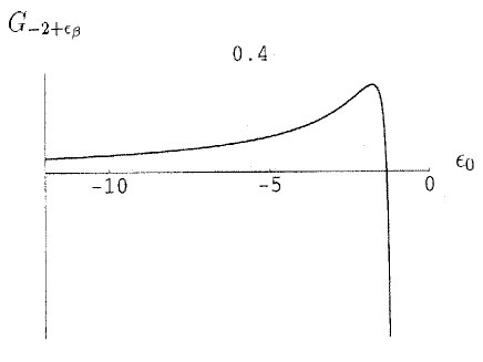
FIG. 1.: $G_{E}(0,0;0,0)$ at $E=-2+\epsilon_{\beta}$, as function of $\epsilon_{0}$. The hybridization is fixed at $\gamma=0.4$.

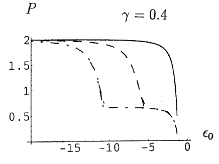
FIG. 2.: The occupancy of the single dot, as function of $\epsilon_{0}$. The curves, from right to left, are for $U$=2, $U=5$, and $U=10$, respectively. The hybridization is fixed at $\gamma=0.4$.

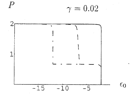
FIG. 3.: The occupancy of the single dot, as function of $\epsilon_{0}$. The curves, from right to left, are for $U$=2, $U=5$, and $U=10$, respectively. The hybridization is fixed at $\gamma=0.02$.

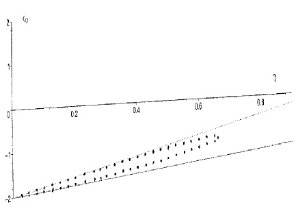
FIG. 4.: $\epsilon_{0}$–$\gamma$ phase diagram for $R=2$. The straight lines which meet at $\epsilon_{0}=-2$ represent the bounds in Eq. (29), between which there exists only one single-electron bound state below the band. Inside the dotted curved line, the system is “metallic”, for $U=\infty$.

FIG. 5.: $\epsilon_{\beta+}$ and $\epsilon_{\beta-}$ as function of $\epsilon_{0}$. Here $R=6$, and the dot is ‘open’: $\gamma=0.98$.

FIG. 6.: The weight of the single-particle wave functions in the bound states on the impurities. Here $R=6$, and the dot is ‘open‘: $\gamma=0.98$.

FIG. 7.: The two single-particle bound state energies below the band, as function of the distance between the impurities.

REFERENCES

- [1] Permanent address: School of Physics and Astronomy, Raymond and Beverly Sackler Faculty of Exact Sciences, Tel Aviv University, Tel Aviv 69978, Israel.
- [2] G. Grabert and M. H. Devoret, eds., Single Charge Tunneling, Coulomb Blockade Phenomena in Nanostructures, NATO ASI, Series B Physics, vol. 294, Plenum, NY (1992); L. P. Kouwenhoven et al., in Mesoscopic Electron Transport, edited by L. L. Sohn, et al., (Kluwer, Dordrecht, The Netherlands, Series E, vol. 345, 105, 1997).
- [3] M. A. Kastner, Rev. Mod. Phys. 64, 849 (1992).
- [4] K. V. Matveev, Phys. Rev. B51, 1743 (1995); A. Furusaki and K. A. Matveev, Phys. Rev. Lett. 75, 709 (1995).
- [5] N. B. Zhitenev, R. C. Ashoori, L. N. Pfeiffer, and K. W. West, Phys. Rev. Lett. 79, 2308 (1997).
- [6] S. Tarucha, D. G. Austing, Y. Tokura, W. G. van der Wiel and L. P. Kouwenhoven, Phys. Rev. Lett. 84, 2485 (2000).
- [7] T. K. Ng and P. A. Lee, Phys. Rev. Lett. 61, 1768 (1988).
- [8] A. Aharony, O. Entin-Wohlman, and Y. Imry, Phys. Rev. B61, 5452 (2000).
- [9] O. Entin-Wohlman, A. Aharony, Y. Imry and Y. Levinson, Europhys. Lett. 50, 354 (2000).
- [10] X. Hu and S. Das Sarma, quant-ph/9911080.
- [11] T. Fujisawa et al., Science 282, 932 (1988).
- [12] F. von Oppen, T. Wettig, and J. Müller, Phys. Rev. Lett. 76, 491 (1996); M. Ortuo and E. Cuevas, Europhys. Lett. 46, 224 (1999).
- [13] This nomenclature is based on the picture of dielectronic donors in a lightly doped semiconductor: having only a single-electron bound state on the donor would mean an ionization of one electron into the conduction band at the transition.
- [14] P. W. Anderson, Phys. Rev. 115, 2 (1959).
- [15] Such an interchange was discussed, in a model without leads, in Ref. [6].
- [16] The same crossover was discussed, for the case without leads, by W. A. Harrison, Phys. Rev. B29, 2917 (1984).