On two continuous models for the dynamics of sandpile surfaces

Abstract

We consider a modified BCRE model for pile surface dynamics and show that in the long-scale limit this model converges to a quasistationary model of pile growth in the form of an evolutionary variational inequality.

I Introduction

Recent much interest to the physics of granular media was, in particular, stimulated by two salient features of the granular state: multiplicity of metastable pile shapes and occurrence of avalanches upon pile surfaces. It has been realized that, to account for metastability, the model of pile surface dynamics should not be written as an evolutionary equation for the pile surface alone. An additional unknown characterizing the flow of grains down the pile surface is useful because such flows are not uniquely determined by the external source and local free surface topography.

A large spatio-temporal scale pile growth model involving two coupled dependent variables and able to account for metastability has been proposed in [1, 2]. This model neglects avalanches as small fluctuations of the pile surface and describes the evolving mean surface of a pile that grows on an arbitrary support under a given distributed source of bulk material. The model permits an equivalent formulation as an evolutionary variational or quasivariational inequality; such a formulation simplifies significantly both the mathematical study of the problem [3] and its numerical solution [1, 4, 5]. As it has been shown in [2], the shapes of real piles on flat open platforms [6] are described by the analytical solutions of this inequality. A modification of the model, able to account for avalanches as almost instantaneous slides, is also discussed in [2]; according to observations made in the same work, such a slide may, indeed, be a possible avalanche scenario (see also [7]).

Independently and using different arguments, the same pile growth model in the form of a variational inequality has been derived by Aronsson, Evans, and Wu [8]. In [9], Evans et al. studied its discontinuous solutions corresponding to avalanches; in [10] Evans and Rezakhanlou showed that the cellular automata models of sandpiles, presented as intuitively attractive examples in almost all works on self-organized criticality [11], converge in a continuous limit to a similar variational inequality with an anisotropy inherited from the cellular structure of these crude models.

A different continuous model, also involving two coupled dependent variables and describing the granular surface flow and pile surface dynamics, has been proposed by Bouchaud, Cates, Ravi Prakash, and Edwards (the BCRE model) [12, 13]. Although the choice of the basic variables in this model is equivalent to that in [1, 2], the model is written for the free surfaces only slightly deviating from the critical slope and employs different phenomenological constitutive relations. The emphasis is put onto the simulation of fast processes, like amplification and distinction of rolling grains population during an avalanche. The BCRE model has been simplified by de Gennes [14], applied to various one-dimensional surface flow problems (see, e.g., [15, 16]), and modified for thick surface granular flows [17]. Further exact solutions to simplified BCRE equations can be constructed by the methods proposed in [18]. Using the BCRE model, Bouchaud and Cates [19] explained another type of avalanches (in a thin granular layer on an inclined plane, see [20]).

Our aim here is to investigate a relation between the two models mentioned above. After reminding briefly the variational and BCRE models, we propose a full-dimensional generalization of the latter, originally formulated by BCRE in the one-dimensional case. To do this, we modify and extend the constitutive relations determining the surface flow velocity and the rolling-to-immobilized-state transition rate: BCRE’s assumption that the slope is everywhere almost critical is too restrictive for our purpose. Rescaling the variables, we show that the modified BCRE model contains a small parameter, the ratio of a characteristic rolling grains layer thickness to the pile size, and hence may often be simplified by employing a quasistationary equation for the rolling grains layer. The issue of scaling turns out to be very important in description of pile growth: another dimensionless parameter in the model thus obtained is the ratio of a typical rolling grain path length to the pile size. For large piles, this coefficient is also small and we show that in the long-scale limit the modified BCRE model tends to the variational model [1, 2]. For small piles, the corresponding term can be significant. These results make clear why differ the shapes of small and large piles and, correspondingly, why different models should be used to simulate, say, formation of large sand dunes and small Aeolian ripples.

II Variational model of pile growth

Let a cohesionless granular material having an angle of repose $\alpha_{r}$ be tipped out onto a given rough rigid surface $y=h_{0}(x)$, where $x=(x_{1},x_{2})\in\mathbb{R}$². We want to find the shape of a pile thus generated.

The real process of pile growth is often intermittent: discharged granular material not only flows continuously over the pile slopes but is also able to build up and then to pour suddenly down the slope in an avalanche. However, the avalanches usually involve only a small amount of particles in a pile and cause small fluctuations of the pile free surface. The model [1, 2] neglects these fluctuations and is a model for the mean surface evolution. Whether the pile evolution is governed by a continuous surface flow or results from many small avalanches, the surface flow is typically confined to a thin boundary layer which is distinctly separated from the motionless bulk [21].

Let us assume for simplicity that the support surface has no steep slopes, i.e.,

$\displaystyle|\nabla h_{0}|\leq k,$

where $k=\tan\alpha_{r}$ (see [1, 2, 3] for the general case). Assuming the bulk density of material in a pile is constant we can write the conservation law as

$\displaystyle\partial_{t}h+\nabla\cdot\mbox{\boldmath$q$}=w,$

where $h(x,t)$ is the free surface, $\mbox{\boldmath$q$}(x,t)$ is the horizontal projection of the flux of rolling particles, and $w(x,t)$ – the source intensity. We neglect the inertia and suppose that surface flow is directed towards the steepest descent,

$\displaystyle\mbox{\boldmath$q$}=-m\nabla h,$

where

$$m(x,t)\geq 0$$ (1)

is an unknown scalar function. The conservation law takes now the form

$$\partial_{t}h-\nabla\cdot(m\nabla h)=w.$$ (2)

It is assumed in this model that the surface slope angle cannot exceed the angle of repose,

$$|\nabla h|\leq k,$$ (3)

and that no pouring occurs over the parts of the pile surface which are inclined less:

$$|\nabla h(x,t)|<k\ \Longrightarrow\ m(x,t)=0.$$ (4)

To complete the model we have to specify the initial,

$$h|_{t=0}=h_{0},$$ (5)

and a boundary condition. Let the granular material be allowed to leave the system freely through part $\Gamma_{1}$ of the boundary of domain $\Omega\subset\mathbb{R}$², and the other part of the boundary, $\Gamma_{2}$, presents an impermeable wall. The boundary conditions are then, respectively,

$$h|_{\Gamma_{1}}=h_{0}|_{\Gamma_{1}},\ \ \ \ m\partial_{n}h|_{\Gamma_{2}}=0.$$ (6)

The model (1)-(6) contains two coupled unknowns, the free surface $h$ and an auxiliary function $m$ determining the rolling grains flux magnitude. Conditions (1), (3), and (4) define $m$ as a multivalued function of $|\nabla h|$, see Fig. 1.

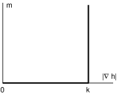
FIG. 1.: Multivalued constitutive relation $m=m(|\nabla h|)$.

The problem (1)-(6) may be considered an anomalous diffusion problem and solved by approximating this highly nonlinear multivalued relation. However, a better way to solve this problem is based on its following reformulation in the form of an evolutionary variational inequality (see [22] and [23] for variational inequalities in mechanics and physics and their numerical solution, respectively).

Let us define the set $K$ of possible surfaces as

$\displaystyle K=\left\{\varphi(x)\ \ \bracevert\ \ |\nabla\varphi|\leq k,\ \ \varphi|_{\Gamma_{1}}=h_{0}|_{\Gamma_{1}}\right\}$

and the scalar product of two functions as $(\phi,\psi)=\int_{\Omega}\phi\psi\,dx$. We can now consider the following problem (variational inequality):

$$\left\{\begin{array}[]{c}Find\text{ \ \ }h(x,t)\text{ \ }such\text{ }that\text{ }h\in K\text{ }for\text{ }all\text{ }t>0,\\ (\partial_{t}h-w,\varphi-h)\geq 0\ \ \mbox{\it for all}\ \varphi\in K,\\ \mbox{\it and}\ h|_{t=0}=h_{0}.\end{array}\right.$$ (7)

Theorem. Function $h(x,t)$ is a solution of the variational inequality (7) if and only if there exists $m(x,t)$ such that the pair $\{h,m\}$ is a solution to (1)-(6).

The outline of the proof is given in [2] (see [3] for mathematical details and a proof of existence of a unique solution to the variational inequality (7)). It has been also shown that the surface flux magnitude $m(x,t)$ is, in this model, a Lagrange multiplier related to the point-wise constraint (3). The values of such multipliers are not uniquely determined by the local conditions, which is the ”mathematical explanation” of long-range interactions typical of extended dissipative systems in a critical (marginally stable) state, see [24].

The model (1)-(6) or, equivalently, (7), has simple analytical solutions [2], such as the conical pile growing under a point-like source or the piles on flat open platforms described in [6]. Numerical solutions [1, 4] also demonstrate simple geometrical structures that agree with one’s sandbox memories. Although this model is much simplified in many respects, it allows for the multiplicity of possible pile shapes. The avalanches may be introduced into the model as solution discontinuities (in time) triggered by sudden changes of the admissible set $K$ [9, 2] and are instantaneous events. On the time scale of a slow pile growth the life of an avalanche is, indeed, very short.

III Modified BCRE equations

The BCRE equations [12, 13] involve two coupled variables: the pile height, $y=h(x,t)$, and the effective thickness (density) of the rolling grains layer, $R(x,t)$ ($R(x,t)d\Omega$ is the volume that the material, currently rolling above the area $d\Omega$, would occupy in the pile). The model has been formulated for a two-dimensional pile ($x\in\mathbb{R}$¹); free surface slope deviations from the critical angle were assumed small. Original BCRE equations included diffusion terms to account for a non-locality of grains dislodgement and for fluctuations of rolling grains velocity. Although diffusion plays a crucial role in BCRE’s scenario of avalanches [12, 13, 19], these terms were regularly omitted by other researchers who either assumed that in their problems diffusion is insignificant and simplified the model, or proposed a different avalanche scenario (see, e.g., [14, 16, 18, 25]). Below, we also omit the diffusion terms at first but introduce small diffusion at a later stage as a means for model regularization in transition to a large-scale limit.

Simplified BCRE equations may be written as follows:

$\displaystyle\partial_{t}h=\Gamma[h,R],\ \ \ \partial_{t}R+\partial_{x}(vR)=w-\Gamma[h,R].$

Here the term $\Gamma[h,R]$ accounts for the conversion of rolling grains into immobilized grains and vice versa, $v$ is the horizontal projection of rolling grains velocity, and $w(x,t)$ is the source intensity (we assume that the tipped grains do not stick to the pile surface but join the rolling grains first).

Limiting their consideration to the slopes that are close to critical, BCRE assumed constant downslope drift velocity $v$. The surface flux magnitude, $q=vR$, is thus determined solely by the rolling layer thickness $R$. Since in the previous model $q=mk$ for the critical slopes, $m$ and $R$ play similar roles and the two choices of basic variables, $\{h,m\}$ and $\{h,R\}$, are essentially equivalent. The exchange term $\Gamma$ in BCRE model is linearized in a vicinity of the critical angle $\alpha_{r}$ and is proportional (for thin surface flows) to $R$: $\Gamma[h,R]=\gamma R(\alpha_{r}-\theta),$ where $\theta(x,t)$ is the surface slope angle and $\gamma$ is a coefficient.

For a three-dimensional pile ($x\in\mathbb{R}$²), the model equations are similar,

$$\partial_{t}h=\Gamma[h,R],\ \ \ \partial_{t}R+\nabla\cdot(\mbox{\boldmath$v$}R)=w-\Gamma[h,R],$$ (8)

but the constitutive relations determining $v$ and, probably, $\Gamma[h,R]$ should be modified; here we will follow [26] (see also [27]). We assume that the rolling particles drift towards the steepest descent of the free surface with a mean velocity $v$ depending on the slope angle (the steeper the slope, the higher is the velocity). On their way downslope, these particles may be trapped and absorbed into the motionless bulk (the steeper the slope, the lower is the trapping rate $\Gamma$). If the surface is horizontal, the mean flow velocity is zero and the trapping rate is maximal, for $\theta=\alpha_{r}$ the rolling particles follow without trapping. Below, we will not consider the overcritical slopes and assume also that the trapping rate is proportional to the amount of rolling grains $R$.

At least partially, this simplified picture can be justified by recent experimental, theoretical, and numerical studies on the motion of a spherical particle on a rough inclined plane [28, 29]. For the relevant region of slope angles $\theta$, the energy dissipation due to the multiple shocks experienced by a moving particle is equivalent to the action of a viscous friction force [28]. Because of that such particles reach a constant mean velocity proportional to $\sin\theta$. Sometimes, however, the particles are suddenly trapped in a well and completely lose their momentum in the direction of motion [29]. Of course, conditions in the collective flow of grains over the pile surface are somewhat different. In particular, the flow velocity may depend on the thickness of rolling grains layer [30] and the exchange rate is not exactly proportional to $R$ [17]. Various improved dependencies can be incorporated into the model. The limiting behavior of the modified BCRE model is, however, robust and does not depend on details. For clarity of presentation we will consider the long-scale limit of a thin-flow model with the simplest phenomenological relations determining the flow velocity and rolling-to-immobilized-state transition.

Since the mean velocity of surface flow is proportional to $\sin\theta$ [28], its horizontal projection $v$ is proportional to $\sin\theta\cos\theta=\tan\theta/(1+\tan^{2}\theta)$. Postulating that the flow is in the steepest descent direction, we obtain $\mbox{\boldmath$v$}=-\mu{\nabla h}/(1+|\nabla h|^{2}),$ where $\mu$ is a coefficient. Simplifying this relation we assume

$$\mbox{\boldmath$v$}=-\mu\nabla h.$$ (9)

The exchange rate $\Gamma$ should not depend on the slope orientation and we assume it to be a smooth decreasing function of $|\nabla h|^{2}$ that becomes zero for critical slopes. Assuming $\Gamma$ is proportional to $R$ (thin flows) we arrive at

$$\Gamma[h,R]=\gamma R\left(1-\frac{|\nabla h|^{2}}{k^{2}}\right)$$ (10)

as the simplest constitutive relation [26]. We will now derive a dimensionless formulation for the modified BCRE model (8)-(10).

The parameters in this model have the following dimensions: $[\gamma]={\cal T}^{-1}$ and $[\mu]={\cal LT}^{-1}$. Let us denote by $\overline{w}$ the characteristic intensity of the external source; $[\overline{w}]={\cal LT}^{-1}$. The three length scales characterizing the pile surface dynamics and surface granular flow may be defined as follows:

• typical thickness of the rolling grains layer, $L_{R}=\overline{w}/\gamma$;

• mean path of a rolling particle before it is trapped strongly depends on the slope steepness but, for a fixed subcritical slope, is proportional to the ratio $L_{P}=\mu/\gamma$ characterizing the competition between rolling and trapping;

• the pile size $L$.

The time $T=L/\overline{w}$ needed for a source with given intensity $\overline{w}$ to produce a pile of size $L$ may be used as a long time scale. Rescaling the variables,

$\displaystyle x^{\prime}=\frac{1}{L}x,\ h^{\prime}=\frac{1}{L}h,\ R^{\prime}=\frac{1}{L_{R}}R,\ w^{\prime}=\frac{1}{\overline{w}}w,\ t^{\prime}=\frac{1}{T}t,$

we arrive at the following dimensionless formulation:

$$\partial_{t}h=\Gamma[h,R],$$ (11)

$$\frac{L_{R}}{L}\partial_{t}R-\frac{L_{P}}{L}\nabla\cdot(R\nabla h)=w-\Gamma[h,R],$$ (12)

$$\Gamma[h,R]=R\left(1-\frac{|\nabla h|^{2}}{k^{2}}\right).$$ (13)

Typically, $L_{R}\ll L_{P}<L.$ The first coefficient in (12) is very small, so it may often be possible to omit the corresponding term and use a quasistationary equation for the rolling layer. Such an approach has already been employed in simulation of the dynamics of sand ripples, see [26]. The second coefficient, $L_{P}/L$, may be significant for small piles, like sand ripples, but becomes small too for large piles. Further simplification of the model is then appropriate.

IV The long-scale limit of BCRE model

Let us denote $\nu=L_{P}/L$ and study the $\nu\rightarrow 0$ behavior of the model (11)-(13). This limit corresponds to the case of large piles ($L\gg L_{P}$). We want to show that in this limit the pile shape evolution is described by the variational inequality (7) which remains invariant under the rescaling employed.

Physically, the situation is clear: although the model (11)-(13) permits grains to roll down upon any inclined slope, the rolling particles are quickly stopped and their paths are short comparing to the pile size for all except the almost critical slopes. This is essentially what is assumed in the model [1, 2] which permits rolling upon the critical slopes only. Mathematically, the situation is somewhat more complicated.

Since $L_{R}\ll L_{P}$, we assume $L_{R}/L$ is $o(\nu)$ and set $L_{R}/L=\nu\lambda(\nu),$ where $\lambda$ tends to zero as $\nu\rightarrow 0$. Let us introduce a new variable, $m=\nu R$, define $\psi(u)=1-u^{2}/k^{2}$, and rewrite the model (11)-(13) as

$$\partial_{t}h=\frac{m\psi(|\nabla h|)}{\nu},\ \ \lambda\partial_{t}m-\nabla\cdot(m\nabla h)=w-\frac{m\psi(|\nabla h|)}{\nu}.$$

For any $\nu>0$ this system consists of two coupled hyperbolic equations. The second equation, which can be regarded as an equation for $m$, contains in its main part the coefficient $\nabla h$ which may be discontinuous. The theory for such equations is complicated and not well developed. To circumvent the difficulty, we add small diffusion to both equations and consider the regularized model

$$\partial_{t}h=\frac{m\psi(|\nabla h|)}{\nu}+\varepsilon_{h}\Delta h,$$ (14)

$$\lambda\partial_{t}m-\nabla\cdot(m\nabla h)=w-\frac{m\psi(|\nabla h|)}{\nu}+\varepsilon_{m}\Delta m,$$ (15)

where the positive coefficients $\varepsilon_{h}(\nu)$ and $\varepsilon_{m}(\nu)$ vanish as $\nu$ tends to zero. It should be noted that, although small diffusion may be physically meaningful and has been included into the original BCRE formulation [12, 13], here we introduce it merely as a parabolic regularization of hyperbolic equations convenient for analyzing the model’s behavior at $\nu\rightarrow 0$.

We assume the same initial and boundary conditions, (5) and (6) correspondingly, for the function $h$. The non-negative values of $m$ both in $\Omega$ at $t=0$ and on the boundary of this domain for $t>0$ may be chosen arbitrary: these initial and boundary conditions result only in the appearance of boundary layers in the solution for any finite $\nu>0$ and are lost in the $\nu\rightarrow 0$ limit. Rigorously, convergence of the problem (14)-(15) to the variational inequality (7) is proved elsewhere [31]. Here we present a simplified scheme of the proof and avoid technicalities.

The main step is, as usual, to obtain uniform in $\nu>0$ a priori estimates on the solutions of the equations (14)-(15). First, taking the gradient and multiplying by $\nabla h$, we derive from (14) a parabolic partial differential equation for $|\nabla h|^{2}$. Since $\psi(k)=0$ and $|\nabla h_{0}|\leq k$, we are able, using the maximum principle for this equation, to show that for $\nu>0$

$$|\nabla h|\leq k\ \mbox{\it for all}\ (x,t);\ h\ \mbox{\it is uniformly bounded.}$$ (16)

Second, using the non-negativeness of the source function $w(x,t)$ and applying the maximum principle to the equation (15), we deduce that for each $\nu>0$

$$m\geq 0\text{\it\ for all }(x,t).$$ (17)

Applying the estimates (16), (17) to the equation (14) we obtain

$$m\psi(|\nabla h|)=O(\nu).$$ (18)

Sending  $\nu$ to zero in (16), (17), (18) we establish the fulfillment in this limit of the conditions (1), (3), and (4). Finally, adding the equations (14) and (15) we obtain

$\displaystyle\lambda\partial_{t}m+\partial_{t}h-\nabla\cdot(m\nabla h)=w+\varepsilon_{h}\Delta h+\varepsilon_{m}\Delta m.$

Since $\lambda$, $\varepsilon_{h}$, and $\varepsilon_{m}$ vanish as $\nu\rightarrow 0$, we can show that the corresponding limits of $h$ and $m$ satisfy also the balance equation (2) in some weak (integral) sense. This completes the proof, because the model (1)-(6) is equivalent to the variational inequality (7).

To illustrate this result we will now compare solutions of the BCRE-type model (14)-(15), solutions of the variational inequality (7), and real shapes of small and large piles. Let us consider the simplest situation: a pile growing under a point source on an infinite horizontal support $h_{0}=0$. Although in this case the piles are known to be almost perfect cones, sometimes one can notice [32] curved tails near the bottom of a small pile (Fig. 2a). As the pile becomes larger, the tail remains of only, say, tens of grain diameters long, so the tail of a large pile is difficult to see (Fig. 2b).

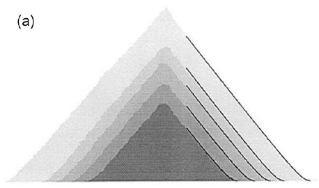
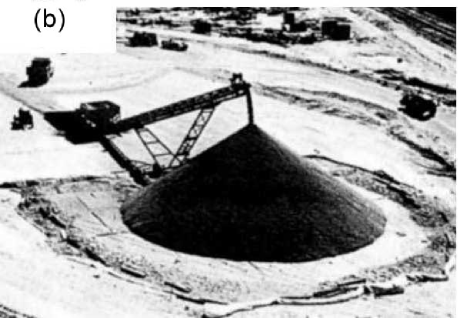
FIG. 2.: Piles growing below a point-like source. (a) Digitized image of a small polenta pile, Alonso and Herrmann [32]. Different gray levels show the pile at different stages of growth, the curved tails near the pile bottom remain short; (b) Large conical pile, photo by Slater [33].

The modified BCRE model (14)-(15) describes this situation quite satisfactory, see Fig. 3. Although the tails of small piles ($\nu=0.2$) are clearly seen, tails of the larger piles ($\nu=0.01$) is difficult to detect. We see also that piles, predicted by the BCRE model with small $\nu$ and $\lambda$, are very close to the growing cone, exact analytical solution of the variational inequality (7). It may be noted that for small values of $\nu$ and $\lambda$ the model equations are stiff and their numerical solution becomes difficult. Thus, even using an implicit finite-difference approximation of (14)-(15), we needed $10^{5}$ time steps in the latter example.

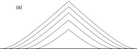
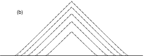
FIG. 3.: Piles growing below a point-like source, numerical solution of (14)-(15) with $\varepsilon_{h}=\varepsilon_{m}=0,\ m|_{t=0}=0,\ \lambda=0.1\nu$, and $k=1$.
(a) Small piles, $\nu=0.2$; (b) Solid line – large piles, $\nu=0.01$; dashed line – analytical solution of the variational inequality (7).

V Conclusion

We considered two different continuous models for the pile surface dynamics: the BCRE model [12, 13] and the variational model [1, 2]. Both models are written for two coupled dependent variables and are able, in principle, to account for multiplicity of metastable pile shapes and surface avalanches. It has been found that the models are related and describe the pile surface dynamics on different spatio-temporal scales.

BCRE-type models may be used to simulate the fast processes, such as the initiation, spreading, and settling down of an avalanche. To describe the much slower dynamics of the mean shape of a pile, the model may often be simplified by employing a quasistationary equation for the rolling grains layer. Such a model is able to predict some peculiarities of small pile shapes [32] and was recently employed for simulating the nonlinear dynamics of sand ripples [26].

Unlike the BCRE models, the variational model of pile growth does not permit the discharged grains to roll upon subcritical slopes and is therefore unable to account for such features of sand surface as sand-ripple instability or surface slope deviation from the critical angle near the bottom of a conical pile. Indeed, these effects are determined by rolling of particles upon the subcritical slopes and are exhibited on the length scale comparable to the mean path of a particle prior to its being trapped.

On the other hand, sand ripples on the dune surface or tiny tails at the bottom of a pile are seen only from a short distance. These small details are difficult to distinguish watching from a larger distance allowing one to follow the evolution of a big dune or formation of a large pile. In such situations the BCRE model contains another small parameter. This complicates simulations and makes them inefficient. As has been shown in our work, in the long-scale limit the BCRE-type models converge to the variational model of pile growth. The latter model is more appropriate for simulating the pile surface dynamics on a large spatio-temporal scale.

REFERENCES

- [1] L. Prigozhin, Zh. Vychisl. Mat. Mat. Fiz. 26, 1072 (1986).
- [2] L. Prigozhin, Phys. Rev. E, 49, 1161 (1994).
- [3] L. Prigozhin, Euro. J. Appl. Math. 7, 225 (1996).
- [4] L. Prigozhin, Chem. Eng. Sci. 48, 3647 (1993).
- [5] T. Elperin and A. Vikhansky, Phys. Rev. E 55, 5785 (1997).
- [6] H. Puhl, Physica A 182, 295 (1992).
- [7] K. Smith, Environmental Hazards (Routledge, London – New York, 1996).
- [8] G. Aronsson, L.C. Evans, and Y. Wu, J. Differ. Equations 131, 304 (1996).
- [9] L.C. Evans, M. Feldman, and R.F. Gariepy, J. Differ. Equations 137, 166 (1997).
- [10] L.C. Evans and F. Rezakhanlou, Commun. Math. Phys. 197, 325 (1998).
- [11] P. Bak, C. Tang, and K. Wisenfeld, Phys. Rev. Lett. 59, 381 (1987).
- [12] J.-P. Bouchaud, M.E. Cates, J. Ravi Prakash, and S.F. Edwards, J. Phys. I France 4, 1383 (1994).
- [13] J.-P. Bouchaud, M.E. Cates, J. Ravi Prakash, and S.F. Edwards, Phys. Rev. Lett. 74, 1982 (1995).
- [14] P.-G. de Gennes, C.R. Acad. Sci., Ser. II-B, 321, 501 (1995).
- [15] T. Boutreux and P.-G. de Gennes, C.R. Acad. Sci., Ser. II-B, 325, 85 (1997);
- [16] P.-G. de Gennes, Avalanches of granular materials, in: R. Behringer and J.T. Jenkins (eds), Powders and Grains 97 (Balkema, Rotterdam, 1997).
- [17] T. Boutreux, E. Raphael, and P.-G. de Gennes, Phys. Rev. E 58, 4692 (1998); P.-G. de Gennes, Physica A 261, 267 (1998); A. Aradian and P.-G. de Gennes, Phys. Rev. E 60, 2009 (1999).
- [18] L. Mahadevan and Y. Pomeau, Europhys. Letters 46, 595 (1999); T. Emig, P. Claudine, and J.-P. Bouchaud, Europhys. Letters, to appear.
- [19] J.-P. Bouchaud and M.E. Cates, Granular Matter 1, 101 (1998).
- [20] A. Daerr and S. Douady, Nature (London) 399, 241 (1999).
- [21] H.M. Jaeger and S.R. Nagel, Science 255, 1523 (1992).
- [22] G. Duvout and J.-L. Lions, Les Inéquations en Mécanique et en Physique (Dunod, Paris, 1972).
- [23] R. Glowinski, J.-L. Lions, and R. Trémolièrs, Analyse Numérique des Inéquations Variationnelles (Dunod, Paris, 1976).
- [24] L. Prigozhin, Free Boundary Problems News, no. 10, 2 (1996).
- [25] S.N. Dorogovtsev and J.F.F. Mendes, Phys. Rev. Lett. 83, 2946 (1999).
- [26] L. Prigozhin, Phys. Rev. E 60, 729 (1999).
- [27] K.P. Hadeler and C. Kuttler, Granular Matter 2, 9 (1999).
- [28] F.-X. Riguidel, R. Jullien, G.H. Ristow, A. Hansen, and D. Bideau, J. Phys. I France 4, 261 (1994); S. Dippel, G.G. Batrouni, and D.E. Wolf, Phys. Rev. E 56, 3645 (1997); C. Henrique et al., Phys. Rev. E 57, 4743 (1998).
- [29] M.A. Aguirre et al., Powder Technology 92, 75 (1997).
- [30] O. Pouliquen, Physics of Fluids 11, 542 (1999).
- [31] L. Prigozhin and B. Zaltzman, in preparation.
- [32] J.J. Alonso and H.J. Herrmann, Phys. Rev. Lett. 76, 4911 (1996).
- [33] R.A. Slater, Stockpiling and Reclaiming Systems, in: M.C. Hawk (ed.), Bulk Materials Handling, v. 1 (University of Pittsbourhg, Pittsbourhg, 1971).